Jirka Slacalek
International Wealth Effects
Discussion Papers
Opinions expressed in this paper are those of the author and do not necessarily reflect views of the institute.
IMPRESSUM © DIW Berlin, 2006 DIW Berlin
German Institute for Economic Research Königin-Luise-Str. 5
14195 Berlin
Tel. +49 (30) 897 89-0 Fax +49 (30) 897 89-200 http://www.diw.de
ISSN print edition 1433-0210 ISSN electronic edition 1619-4535
JIRKA SLACALEK
German Institute for Economic Research, DIW Berlin
June 12, 2006 E-mail: [email protected]
Web: http://www.slacalek.com/
Abstract. This paper investigates the wealth effect for 16 indus-trial countries using the recently proposed technique that exploits the sluggishness of consumption growth. I estimate that the long-run marginal propensity to consume from wealth varies from less than 0.5 cents in France to 4.5 cents in the US. I document that the wealth effect tends to be larger in countries with more developed financial markets and has decreased in the last twenty years.
Keywords: wealth effect, income effect, consumption dynamics, sticky information.
JEL classification: E21, E32, C22
1. Introduction
Household’s wealth is a major determinant of consumption expen-diture. The magnitude of the reaction of consumption to changes in wealth, the wealth effect, depends on a number of factors, including consumers’ preferences, interest rate, and institutional setting of the financial markets (e.g. liquidity constraints and the costs of trading fi-nancial assets). While a number of recent papers (Bertaut, 2002; Byrne and Davis, 2003; Fernandez-Corugedo et al., 2003; Pichette and Trem-blay, 2003; Catte et al., 2004; Lettau and Ludvigson, 2004, Hamburg et al., 2005 and others) attempt to analyze theoretically and estimate empirically the magnitude of the wealth effect in individual countries, a Jirka Slacalek, German Institute for Economic Research, DIW Berlin, Depart-ment of Macro Analysis and Forecasting, K¨onigin-Luise-Strasse 5, 14195 Berlin, Germany. Financial support from the European Commission’s DG Research, con-tract #SCS8–CT–2004–502642 is gratefully acknowledged. I thank Christopher Carroll, Ray Barell and Boriss Siliverstovs for helpful suggestions and comments. I thank various seminar audiences for feedback and Carol Bertaut, Amanda Choy, Nathalie Girouard and Roberto Golinelli for data and help in constructing the dataset used in the paper.
systematic cross-country analysis is still lacking. This paper presents a comparative analysis of the wealth effect and its determinants in major industrial countries.
Research in this area was spurred by two factors. First, the stock market booms of 1990s stimulated policy-makers’ and academics’ in-terest in whether and how economic policies should respond to asset price movements. A necessary pre-requisite for designing appropriate policies in presence of “excessive” stock and housing price movements and bubbles is the ability to evaluate the effects of these movements on the real economy. Two major channels were identified in the litera-ture: the effect of stock prices on consumption—which is in the focus of this paper—and the effect on firms’ investment expenditure. The quantitative estimation of these effects was made possible by the the second essential factor: the developments in time series econometrics methods that deal with unit roots and cointegration.
This paper estimates the wealth effect using a methodology for an-alyzing the wealth effect based on the sluggishness of consumption growth has recently been developed by Carroll (2004) and Carroll et al. (2006). The technique incorporates some features that recent literature (including Fuhrer, 2000 and Sommer, 2002) suggests are important for capturing the aggregate consumption dynamics, including inattentive-ness/habit formation of consumers and measurement error in consump-tion data. Unlike the frequently-used cointegraconsump-tion methodology, the Carroll approach does not require long spans of stable data.
Almost all papers that estimate the wealth effect assume that there exist a stable, valid cointegrating relationship between consumption, income and wealth. However, as has recently been noticed, this coin-tegration methodology is vulnerable to some theoretical and empirical attacks. The theoretical justification for the cointegration approach is based on the log-linear approximation of consumer’s intertemporal budget constraint. Unfortunately, there is no reason to expect that the parameters that are required for the approximation to be valid (long-run productivity growth and interest rate) are actually stable over the long enough time frames necessary to identify the cointegrating rela-tionship. It is because the cointegration methodology has to pin down long-run relationships that structural instability (documented in Hahn and Lee, 2001; Rudd and Whelan, 2002; and Slacalek, 2004) may cause some serious problems.
This paper analyzes the effect of household wealth on consumption. I compare the estimates of the wealth effects implied by the two method-ologies: the traditional cointegration technique and a new approach based on the sluggishness of consumption growth. I also investigate
the determinants of the wealth effect and the evolution of its size over time. My results indicate that the new technique implies somewhat smaller magnitude of the wealth effect in the G-8 countries: the long-run marginal propensity to consume from wealth varies from less than 0.5% in France to 4.5% in the US. In contrast, that methodology im-plies a larger size of the income effect. In addition, I document that the wealth effect tends to be larger in countries with more developed financial markets and has decreased in the last twenty years.
The plan of the paper is as follows. Section 2 outlines the Euler equation-based approach recently proposed by Carroll (2004) and Car-roll et al. (2006). Section 3 summarizes the traditional cointegration methodology for estimating the wealth effect. Section 4 presents em-pirical estimates of the wealth effect and income effects. Section 5 at-tempts to track down some factors that influence the magnitude of the wealth effect. Finally, section 6 concludes and the Appendix presents some additional information on the dataset used in the paper.
2. Methodology Based on the Sluggishness of
Consumption Growth
2.1. Intermezzo: A Brief History of Aggregate Consumption Dynamics. Before summarizing the Carroll’s (2004) methodology to estimate the wealth effect I will outline some recent developments in the theory of aggregate consumption dynamics.
Robert Hall (1978) showed that consumption of a household with time separable utility and no precautionary saving motive follows a random walk. However, several researchers (including Flavin, 1981; Campbell and Mankiw, 1989; and Carroll et al., 1994) have argued since that random walk is not an adequate approximation of the ag-gregate household consumption. Their work documents a number of “excess sensitivity” puzzles: contrary to the Hall theory, future con-sumption growth was shown to be significantly affected by past vari-ables (including lagged income, consumption and consumer sentiment). A number of economists suggested possible solution to the excess sensitivity puzzles. Campbell and Mankiw (1989) propose a model with a fraction of income going to the “rule of thumb” consumers who consume all their current incomes. Bacchetta and Gerlach (1997) sug-gest that consumption of liquidity constrained agents will be predicted with past fluctuations in various credit aggregates (such as mortgage and consumer credits).
Excess sensitivity of consumption growth to its lags can be explained if consumers are habit forming, with their current utility depending on
past consumption, rather than being time-separable (see e.g. Muell-bauer, 1988). Sommer (2002) advances this argument and reports that the US aggregate consumption dynamics is adequately captured with two ingredients: habits and measurement errors. Sommer’s (2002) con-sumers maximize a utility function with additive habits,
max {Cs} Et ∞ X s=t δs−tU(Cs−λCs−1)
subject to the standard budget constraint. Dynan (2000) showed that the Euler equation for this objective function with a CRRA outer utility can be approximated by
∆ logCt=µ0 +λ∆ logCt−1+εt. (1)
Sommer (2002) proposes an econometric technique to estimate this equation based on instrumental variables. Sommer’s (2002) method is robust to the existence of measurement error in observed consumption data and wipes out most of the excess sensitivity in the US consump-tion.
While there is much evidence for the existence of positive autocor-relation in consumption growth in macro data (both in the US and elsewhere; see Fuhrer, 2000; Sommer, 2002; Carroll and Slacalek, 2006 and Carroll et al., in progress), the results for micro data are rather mixed (for example Dynan, 2000 finds no evidence of habit formation in the PSID micro data on food consumption). This is not consistent with the habit-formation model, which predicts positive autocorrelation in consumption growth in micro, as well as in macro data.
To reconcile this puzzle, Carroll and Slacalek (2006) offer an alter-native interpretation of the Euler equation (1). Carroll and Slacalek show that aggregating consumers with time separable utility who up-date their information about aggregate variables occasionally rather than instantaneously results in equation almost identical to (1) on the aggregate level.1 The consumption path of individual consumers, how-ever, follows random walk and consequently the consumption growth observed in micro data lacks autocorrelation.
The empirical estimation of the Euler equation (1) is complicated by some issues that require further discussion. First, several authors (Wilcox, 1992; Bureau of Economic Analysis, 2002; Sommer, 2002) document that a large component in consumption data (around 30% of the PCE in the US, likely even more abroad) is estimated, imputed
or interpolated. Consequently, the published consumption data dif-fer from the (unobservable) “true” ones due to a sizable measurement error.
The presence of this measurement error complicates the estimation and inference about the consumption Euler equations. It is well known that if a regressor is measured with iid error, the OLS estimate of its coefficient is biased toward zero. In our case it turns out that the measurement error occurs in the level of consumption but the Euler equations actually relate consumption changes. As shown by Sommer (2002), in such a situation, the measurement error in the Euler equation (1) will have a possibly quite complicated structure with (substantial negative) serial correlation,
∆ logCt=µ0+λ∆ logCt−1+vt+θ1vt−1+θ2vt−2.
Sommer proposes that a consistent estimator of λ can be obtained from the instrumental variables regression if instruments are lagged the appropriate number of periods (to mitigate the correlation between the measured consumption growth and disturbances).
2.2. The New Methodology Based on the Sluggishness of Con-sumption Growth. Carroll (2004) and Carroll et al. (2006) propose a new, alternative method to estimate the magnitude of the wealth ef-fect. The starting point for the Carroll’s (2004) technique is the Euler equation (1),
∆ logCt=µ0 +λ∆ logCt−1+εt.
The two most important shocks to consumption growth are probably due to unexpected changes in income and wealth. Suppose the distur-bance term is decomposed into a part due to the current changes in household income, wealth and the rest,εt =αy∆ logYt+αw∆ logWt+
ηt. The coefficients αy and αw are the immediate responses of con-sumption growth to (unexpected) income and wealth growth, respec-tively. Analogously, the effect of one percentage point increase in wealth growth at time t−s on consumption growth is αwλs. Finally, the long-run (cumulative) effects of income and wealth are the sums of these partial effects, αy
P∞
i=0λi =αy/(1−λ) and αw/(1−λ), respec-tively. To identify the magnitudes of the income and wealth effects, Carroll and Otsuka iterate on the Euler equation backward,
where ˜µk =µ0×(1−λk)
±
(1−λ). This equation can be rewritten (for
k >2) as
∆ logCt−λk∆ logCt−k= ˆµk+ k−1
X
i=2
λi¡αy∆ logYt−i+αw∆ logWt−i
¢ +˜ηk,t, (2) where ˜ηk,t =εt+λεt−1+ Pk−1 i=2 λiηt−i.
Carroll and Otsuka (2004) propose the following procedure to esti-mate the impact of wealth on consumption.
• Estimateλin equation (1) using IV (with appropriately lagged instruments).
• Estimate αw and αy in equations (2) for k = 3,4 and 5 after imposingλ from step 1.
• Transformαs to obtain estimates of the short-run and long-run
MPCWs, MPCSR
w and MPCLRw , and marginal propensities to consume from income (MPCY), MPCSRy and MPCLRy .
Due to measurement error that causes the regressors and error terms to be correlated for k = 1 and 2 equations (2) are estimated only for
k >2.
The Euler equation approach adopts a two-step estimation proce-dure to identify the consumption growth persistence parameter λ and the immediate propensities to consume from wealth and incomeαw and
αy. The technique is justified once λ in the first step can be reliably identified (which we manage for almost all countries). Second, to in-crease the efficiency of the estimates ofαs, equation (2) is estimated as a system fork = 3,4 and 5 rather than a single regression. This results in more precise estimates of the MPCs and seems to be justified by the diagnostics tests in which αs in the individual equations (for k = 3,4 and 5) turn out to be very similar. These issues are discussed further in section 4 below.
3. Wealth Effects: Cointegration Methodology
The traditional, cointegration methodology for estimating the wealth effect is based on the assumption that there exists a valid and sta-ble cointegrating relationship between consumption, labor income and wealth. If that is correct, an estimate of βa in the regression
gives the percentage response of consumption to one percentage point change in wealth.2 The marginal propensity to consume from wealth (MPCW), the dollar response of consumption to a one-dollar increase in wealth, is then obtained as MPCw = βa× C/A, where C/A is a recent value of the consumption–wealth ratio.3
3.1. Theoretical Justifications for the Cointegration Method-ology. Lettau and Ludvigson (2001) and Lettau and Ludvigson (2004) attempt to provide a theoretical justification for the cointegrating re-gressions (3) based on the log-linear approximation of consumer’s in-tertemporal budget constraint.4 Consumer’s budget constraint is
Wt+1 =Rt+1(Wt+Yt−Ct), (4) whereRt+1 is the rate of return on saving between timet andt+ 1 and
Wt is total household wealth including human wealth. Campbell and Mankiw (1989) approximate the intertemporal budget constraint with
logCt−logWt =Et ∞
X
i=1
ρi(r
t+i−∆ logCt+i), (5)
where rt+i = log(1 +Rt+i) and ρ is a parameter between 0 and 1 (ρ = 1−exp(log(C/W)) and log(C/W) is the log of the steady state consumption–wealth ratio). The approximation (5) was obtained tak-ing the Taylor series expansion of (4), impostak-ing a transversality condi-tion and taking expectacondi-tions. A complicacondi-tion with the expression (5) is that the wealthWtconsists from financial wealth and unobservable hu-man wealth Ht=Et
P∞
j=0Yt+j
± Qj
i=0Rit+i. This difficulty is overcome by postulating that human capital is proportional to current income. In other words, the following log-linear approximation to human wealth should hold, logHt = κ+ logYt+vt, where κ is a constant and vt is a zero mean, stationary variable. Finally, combining this expression with approximations (5) and logWt ≈(1−ν) logAt+νlogHt (where
ν = 1−A/W is the steady-state ratio of nonhuman to total wealth)
2Equation (3) uses the following notation: Ctis consumption,Atis net household
wealth (net worth) andYtis labor income.
3One issue about this estimate of MPCW is that theC/Aratio is not stationary.
We report the cointegration-based estimates here for comparison with much of the literature on the wealth effect.
yields
logCt−βalogAt+βylogYt≈Et ∞
X
i=1
ρi¡(1−ν)r
t+i−∆ logCt+i+ν∆ logYt+i+1
¢ .
(6) If the right-hand side of equation (6) is stationary, this approximation provides rationale for estimating cointegrating regressions such as (3). 3.2. Shortcomings of the Cointegration Methodology. The prob-lems with the cointegration methodology fall into two broad areas: (i) the above theoretical derivations and (ii) the empirical implementation of the cointegrating regression.
As pointed out by Carroll and Otsuka (2004), there is no reason for the approximation (6) to provide a satisfactory approximation to the budget constraint if some of the variables assumed to be stationary are not. In particular, the approximations in LL, such as (6), are not valid if there are permanent changes in the productivity growth rate, and their validity is doubtful even if productivity growth is highly seri-ally correlated. Empiricseri-ally, there is strong evidence for the persistent changes in the mean of productivity growth in the US. The average US productivity growth was almost twice as high before 1973 and after 1995 compared to the 1973–1995 period.5
The empirical evidence for the existence of a stable cointegrating relationship is mixed. Rudd and Whelan point out that there are two problems with the way Lettau and Ludvigson (2004), LL, construct data. First, LL deflate the consumption series with a different deflator from labor income and wealth. The consumption series is deflated with the nondurables and services (NDS) deflator. The wealth and labor income series, in contrast, are deflated using the deflator for total personal consumption expenditure (PCE). This appears to be an error in LL’s treatment of the data, since economic theory provides no reason to deflate the dependent and independent variables by different price indexes. Second, Rudd and Whelan claim that the consumption series LL use, consumption of nondurables and services excluding expenditure on shoes and clothing, is not consistent with the wealth series. Rudd and Whelan argue that the right measure of consumption to use in this application the total personal consumption expenditure.
Hahn and Lee (2001) find evidence for structural instability; Lettau and Ludvigson (2004) on the other hand argue that the cointegration
5The average productivity growth in the non-farm business sector was 2.7% in
is stable. Rudd and Whelan (2002) argue that when the series are con-structed appropriately there is no evidence for cointegration in the US data. Slacalek (2004) finds little evidence for the stable cointegration between consumption, income and wealth in international data.
4. Empirical Results
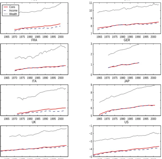
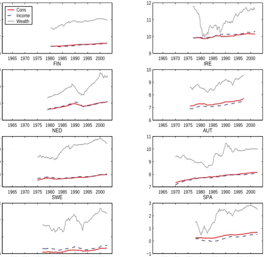
This section presents the estimates of the wealth effects in recent quarterly data from 16 industrial countries.6 The data for G-8 coun-tries, defined as Australia, Canada, France, Germany, Italy, Japan, the UK and the US, are shown in Figure 1; those for the remaining (“small”) countries, Austria, Belgium, Denmark, Finland, Ireland, the Netherlands, Spain and Sweden, are displayed in Figure 2.
The data indicate that the low-frequency movements in consumption closely track down the movements in income. The wealth series, in contrast, tends to be more volatile than both income and consumption. As expected, income is somewhat more volatile than consumption—an intuitive and well-known finding that documents that agents smooth their consumption paths. The wealth–consumption ratios are in the range of 5–13 for G-8 countries, except for the UK where the W– C ratio recently reached about 25. Similarly, in small countries the wealth–consumption ratios are about 5–10, except for Belgium and the Netherlands with the W–C ratios of roughly 15.
The following technology was adopted for the baseline estimation results, shown in Table 1 and Figure 3. First, for each country, con-sumption growth persistence λ was estimated using the IV regressions with the following instruments: real three-month interest rate, wealth growth, unemployment and lagged consumption. In countries where the instruments were not strong enough to warrant reliable estimation of consumption growth persistence—Australia, Belgium, Finland and Austria—λ was imposed to be 0.75. A number of studies (Carroll, 2003; Reis, 2004; Carroll and Slacalek, 2006; Carroll et al., in progress) find this is a reasonable value of the speed at which consumers update their information. The adequate quality of instruments was measured with the first stage F statistics greater than 5.7
Second, given λ, following Carroll and Otsuka (2004), three alterna-tive models of equation (2) were estimated for each country.
6See the Appendix for a description of data.
7Admittedly, the first stage F statistics are in some cases lower than the
bench-mark value of 10 suggested by Stock et al. (2002). However, the Moreira (2003) confidence intervals robust to weak instruments suggest that the usual standard errors approximate well the uncertainty aboutλin this application for all countries except Belgium.
Figure 1. Consumption, Wealth and Income: G8 Countries 1965 1970 1975 1980 1985 1990 1995 2000 9 10 11 12 AUS Cons Income Wealth 1965 1970 1975 1980 1985 1990 1995 2000 7 8 9 10 11 CAN 1965 1970 1975 1980 1985 1990 1995 2000 0 1 2 3 4 FRA 1965 1970 1975 1980 1985 1990 1995 2000 0 1 2 3 GER 1965 1970 1975 1980 1985 1990 1995 2000 0 1 2 3 4 ITA 1965 1970 1975 1980 1985 1990 1995 2000 5 6 7 8 9 JAP 1965 1970 1975 1980 1985 1990 1995 2000 −8 −6 −4 −2 UK 1965 1970 1975 1980 1985 1990 1995 2000 −5 −4 −3 −2 −1 US
Note: The figure shows logs of real per capita consumption, income and wealth. (1) Model 1 (M1): Equation (2) is estimated with ∆ logCt, ∆ logWt
and ∆ logYt.
(2) Model 2 (M2): Equation (2) is estimated with dCt, dWt and
dYt (defined below) in place of ∆ logCt, ∆ logWt and ∆ logYt. (3) Model 3 (M3): Equation (2) is estimated with dCt and unex-pected parts ofdWtanddYt,dWt−Et−1dWtanddYt−Et−1dYt. The expectations Et−1dYt and Et−1dYt are approximated as one-period ahead forecasts ofdWtand dYt from the regressions of these variables on a constant,dWt−1 and dYt−1.
The rationale for the three models is as follows. The parameters αy and αw in equation (2) are by themselves not measures of the mar-ginal propensities to consume from income and wealth. To obtain the
Figure 2. Consumption, Wealth and Income: Small Countries 1965 1970 1975 1980 1985 1990 1995 2000 0 2 4 6 BEL Cons Income Wealth 1965 1970 1975 1980 1985 1990 1995 2000 9 10 11 12 DEN 1965 1970 1975 1980 1985 1990 1995 2000 7 8 9 10 FIN 1965 1970 1975 1980 1985 1990 1995 2000 6 7 8 9 10 IRE 1965 1970 1975 1980 1985 1990 1995 2000 7 8 9 10 11 NED 1965 1970 1975 1980 1985 1990 1995 2000 7 8 9 10 11 AUT 1965 1970 1975 1980 1985 1990 1995 2000 10 11 12 13 SWE 1965 1970 1975 1980 1985 1990 1995 2000 −1 0 1 2 3 SPA
Note: The figure shows logs of real per capita consumption, income and wealth.
MPCYs and the MPCWs one has to do one of the following. Either multiply αs with the most recent consumption–wealth (consumption– income) ratio, or estimate equation (2) with dCt = (Ct−Ct−1)/Ct−6,
dYt = (Yt − Yt−1)/Ct−6 and dWt = (Wt − Wt−1)/Ct−6 rather than ∆ logCt, ∆ logYt and ∆ logWt, respectively. The estimates of αs and
α/(1−ρ)s from these “transformed” regressions are then the appropri-ate estimappropri-ates of short- and long-run MPCs. The former method was adopted in model M1, the latter in model M2. Model M3 attempts to capture the idea that the correct measure of income shocks to look at is theunexpected shocks, rather than the actual changes in income and wealth.
Some comments on the estimation strategy are in order. First, the number of regressions, k = 3,4,5 was chosen somewhat arbitrarily. I experimented with adding additional regressions (k = 7 and 8); the results are not sensitive to this. Second, all three models were estimated fork = 3,4,5 using seemingly unrelated regression (SUR) withαs being restricted to be the same across the three equations. Statistically, the data seem to like this restriction in that the p values of the test of this restriction are always very high (around 0.3). Third, the consumption at time t−6 in the denominator of the transformed regressors serves as the initial consumption level since the earliest consumption level among the regressors is 6.
The estimation results with the MPCWs implied by the baseline specification are shown in Table 1. The third column displays the estimated consumption growth persistence, λ. The consumption per-sistence parameter tends to be close to 0.7 (the average of λs across all countries is 0.66). Obviously, the precision of the estimates of λ
varies across countries; λcan be pinned down very well for the US, less well for some other countries. A typical HAC robust standard error for λ is about 0.15–0.20. The precision of λ depends on (at least two factors): the quality of instruments and the amount of measurement error in consumption data. The first stage F statistics, measuring the quality of instruments are overwhelmingly significant for most countries (Australia, Austria, Belgium and Finland being the exceptions).
The fourth column shows the estimates of αw in (2) for model M1. Columns 5–9 display the implied short- and long-run wealth effects for models M1–M3. Finally, the last column shows for comparison the estimate of the (long-run) wealth effect implied by the cointegration methodology. The first two lines in Table 1 compare the results for two alternative measures of household wealth in the US, net worth (consisting of net financial wealth and net tangible assets) and net financial wealth.8 The estimates of MPCLR
w for the US for the two
measures of wealth are almost identical; they indicate the long-run MPCW of 4–4.5%.
The Euler approach estimates of MPCW for other countries range between 0.3 and 4.5%. Compared to other countries, the MPCWs are substantially bigger in the US and particularly in Australia. Surpris-ingly, the estimates imply relatively low values of MPCW for the UK and the Netherlands. This may be caused by relatively high wealth– consumption ratios in these two countries.
8The results in the first line with the net worth measure of wealth are replications
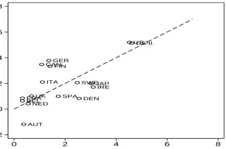
Figure 3. Alternative Estimates of the MPCLRw : Car-roll and Otsuka (2004) vs. Cointegration Methodology
US I.US II. CAN FRA GER ITA JAP UK BEL DEN FIN IRE NED AUT SWE SPA −2 0 2 4 6 8 MPCW Coint 0 2 4 6 8 MPCW C&O
Note: Comparison of estimates of MPCLRw of Table 1, models M3 and CI. The
dashed line is the 45 degree line.
The Euler approach estimates of MPCW for the three models tend to be similar across countries. As expected, the MPCLR
w in a number
of countries is a bit higher than that for M2, reflecting the fact that consumers should react to unexpected shocks to income more than when certain portion of shocks is expected.
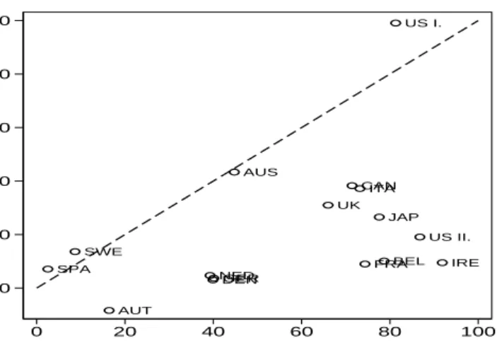
Figures 3 and 4 present scatter plots of estimates of MPCLR
w from the Euler equation (model M3) and cointegration methodologies together with the 45 degree line. The points in the scatter plot tend to lie relatively close to the 45 degree line, implying that the two estimation methods often produce similar values of MPCLRw . However, as shown in Figure 4, the cointegration methodology tends to overstate the MPCW for the G-8 countries.
Table 2 presents estimates of the wealth effect for an alternative specification, in whichλwas imposed to be 0.75 for all countries, rather than estimated. This seems to change the results a bit, in particular for the countries where the estimated λ is different from 0.75, such as Germany and France. Overall, for most countries it however, does not substantially affect the findings.
Table 3 summarizes the estimates of the marginal propensities to con-sume from income, MPCY. Judging by the spread in alternative model estimates (M1–M3) these are harder to pin down than the MPCWs. Overall, the cointegration-based MPCY tend to be smaller than the Euler-based MPCY, as documented in Figure 5. A typical value of the
Figure 4. Alternative Estimates of the MPCLRw : Car-roll and Otsuka (2004) vs. Cointegration Methodology, G8 Countries US I.US II. CAN FRA GER ITA JAP UK 0 2 4 6 8 MPCW Coint 0 2 4 6 8 MPCW C&O
Note: Comparison of estimates of MPCLRw of Table 1, models M3 and CI. The dashed line is the 45 degree line.
Figure 5. Alternative Estimates of the MPCLR
y :
Car-roll and Otsuka (2004) vs. Cointegration Methodology
US I. US II. AUS CAN FRA GER ITA JAP UK BEL DEN IRE NED AUT SWE SPA 0 20 40 60 80 100 MPCY Coint 0 20 40 60 80 100 MPCY C&O
Note: Comparison of estimates of MPCLRy of Table 3, models M3 and CI. The
dashed line is the 45 degree line.
long-run MPCY implied by the cointegration methodology is around 30%, while the Euler methodology generates estimates of MPCLR
y of about 75%.
Figure 6. MPCW vs. Enforcement of Contracts, Num-ber of Procedures US US II. CAN FRA GER ITA JAP UK BEL DEN FIN IRE NED AUT SWE SPA 0 1 2 3 4 MPCW (%) 10 15 20 25 30 Enf of Contracts
Enforcement of Contracts, Number of Procedures
Figure 7. MPCW vs. Share of Top 10 Banks Controlled by Government US US II. CAN FRA GER ITA JAP UK BEL DEN FIN IRE NED AUT SWE SPA 0 1 2 3 4 MPCW (%) 0 20 40 60 80
Top 10 Banks Controlled by Government
Share of Top 10 Banks Controlled by Government
5. What Determines the Wealth Effect?
5.1. Institutional Determinants. Figures 6 and 7 show some ev-idence that the wealth effects tend to be stronger in countries with better functioning financial market infrastructure and overall institu-tional setting. Figure 6 displays a negative relationship between the size of the wealth effect and number of procedures necessary to en-force contracts (a measure of quality of country’s legal system). Figure 7 documents that the wealth effects are typically smaller in countries
with high share government-owned banks. This can in turn be related to the quality of country’s banking and financial system.
5.2. Has the Wealth Effect Changed Recently? Table 4 compares the estimates of the wealth effect for pre- and post-1985 periods (for a subset of countries, G-6). The long-run marginal propensity to con-sume from wealth has fallen in most countries after 1985. It is now on average almost three times smaller than it was in the pre-1985 period. One explanation for this finding may be that the global financial mar-kets have recently become more interdependent and in particular more volatile. At the same time, financial markets are now, arguably, also more efficient, which makes it possible for the households to smooth consumption more efficiently. Consequently, consumption is now less responsive to a unit fluctuation in wealth than they were in the past.
5.3. What is the Relevant Measure of Wealth? The right mea-sure of household wealth to be used in estimating the wealth effect is the net household wealth. However, due to difficulties in obtaining long enough household wealth data, some authors proxy household wealth with stock prices. Intuitively, stock prices will not be a very good proxy of household wealth in countries with low stock market capitalization and in countries where households hold only a small fraction of their wealth in stocks.
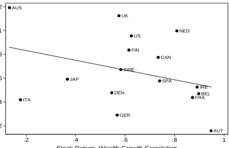
Figures 8 and 9 compare the movements in household wealth and stock prices in G-8 and small countries. Correlation between stock price growth and wealth growth is positive but not extremely strong, 0.63 averaging across countries. Figure 10 shows a scatter plot of this correlation and stock market capitalization. Interestingly, the rela-tionship, if anything, is negative—correlation tends to be weaker for countries with high stock market capitalization.
Relatively low correlation between stock returns and wealth growth suggest that the regressions that use stock prices as a proxy for house-hold wealth are subject to substantial measurement error. Correspond-ingly, in such regressions the estimates of the wealth effect are biased toward zero. This in fact turn to be the case in cointegrating regres-sions of consumption on stock prices and income (not reported here), in which the estimates of MPCLRw tend to be smaller by 1-2% than when the appropriate wealth series is used. The estimates of MPCW from
Figure 8. Wealth and Stock Prices: G8 Countries 1965 1970 1975 1980 1985 1990 1995 2000 2 2.5 3 3.5 4 4.5 5 5.5 6 AUS 1965 1970 1975 1980 1985 1990 1995 2000 10.6 10.8 11 11.2 11.4 11.6 11.8 12 Wealth Stock Prices 1965 1970 1975 1980 1985 1990 1995 2000 2 2.5 3 3.5 4 4.5 5 5.5 6 CAN 1965 1970 1975 1980 1985 1990 1995 2000 9.6 9.8 10 10.2 10.4 10.6 10.8 11 1965 1970 1975 1980 1985 1990 1995 2000 4 5 6 7 8 FRA 1965 1970 1975 1980 1985 1990 1995 2000 2 2.5 3 3.5 4 1965 1970 1975 1980 1985 1990 1995 2000 2 2.5 3 3.5 4 4.5 5 5.5 6 GER 1965 1970 1975 1980 1985 1990 1995 2000 1.6 1.8 2 2.2 2.4 2.6 2.8 3 1965 1970 1975 1980 1985 1990 1995 2000 0 5 ITA 1965 1970 1975 1980 1985 1990 1995 2000 2 3 4 1965 1970 1975 1980 1985 1990 1995 2000 0 1 2 3 4 5 6 JAP 1965 1970 1975 1980 1985 1990 1995 2000 6 6.5 7 7.5 8 8.5 9 1965 1970 1975 1980 1985 1990 1995 2000 0 1 2 3 4 5 6 UK 1965 1970 1975 1980 1985 1990 1995 2000 −4.5 −4 −3.5 −3 −2.5 1965 1970 1975 1980 1985 1990 1995 2000 2 4 6 US 1965 1970 1975 1980 1985 1990 1995 2000 −2
Note: Comparison of log real per capita wealth and log stock prices.
these regressions are substantially smaller than the estimates of cointe-grating regressions of consumption on wealth and income.9 The caveat from this exercise is that it is important to use the appropriate mea-sure of household wealth when estimating the marginal propensities to consume.
6. Conclusion
This paper compares two alternative methods to estimate the mar-ginal propensities to consume from wealth and income for a panel of
9While the measurement error bias in cointegrating regressions is asymptotically
negligible (because the estimates are super-consistent), it may still be relevant in the relatively small samples available for analysis.
Figure 9. Wealth and Stock Prices: G8 Countries 1965 1970 1975 1980 1985 1990 1995 2000 4 6 BEL 1965 1970 1975 1980 1985 1990 1995 2000 −2 −1 0 Wealth Stock Prices 1965 1970 1975 1980 1985 1990 1995 2000 2 4 6 DEN 1965 1970 1975 1980 1985 1990 1995 2000 6 8 1965 1970 1975 1980 1985 1990 1995 2000 4 5 6 7 8 9 10 FIN 1965 1970 1975 1980 1985 1990 1995 2000 3.5 4 4.5 5 5.5 1965 1970 1975 1980 1985 1990 1995 2000 0 2 4 6 IRE 1965 1970 1975 1980 1985 1990 1995 2000 3.5 4 4.5 5 1965 1970 1975 1980 1985 1990 1995 2000 2 4 6 NED 1965 1970 1975 1980 1985 1990 1995 2000 6 1965 1970 1975 1980 1985 1990 1995 2000 3 3.5 4 4.5 5 5.5 6 AUT 1965 1970 1975 1980 1985 1990 1995 2000 3 3.5 4 4.5 5 5.5 6 1965 1970 1975 1980 1985 1990 1995 2000 0 5 SWE 1965 1970 1975 1980 1985 1990 1995 2000 8 1965 1970 1975 1980 1985 1990 1995 2000 3 4 5 6 7 SPA 1965 1970 1975 1980 1985 1990 1995 2000 −5 −4 −3 −2 −1
Note: Comparison of log real per capita wealth and log stock prices.
industrial countries. The traditional cointegration methodology esti-mates the MPCs based on the coefficients from cointegrating regres-sions of consumption on income and wealth. The alternative methodol-ogy is based on the sluggishness of consumption growth. The long-run marginal propensities to consumes from wealth range from 0.3% to 4.5%; the short-run MPCWs are about four times lower. The (long-run) marginal propensities to consume from income are about 60%. The MPCWs tend to be greater for countries with better functioning institutional setting and appear to have fallen in the last twenty years.
Figure 10. Correlation between Stock Returns and Wealth Growth vs. Stock Market Capitalization
US AUS CAN FRA GER ITA JAP UK BEL DEN FIN IRE NED AUT SWE SPA .2 .4 .6 .8 1 1.2
Stock Market Capitalization
.2 .4 .6 .8 1
Stock Return−Wealth Growth Correlation
Note: Stock market capitalization is measured as a fraction of GDP in 2003. References
Bacchetta, Philippe, and Stefan Gerlach (1997), “Consumption and Credit Con-straints: International Evidence,”Journal of Monetary Economics, 40, 207–238. Bertaut, Carol (2002), “Equity Prices, Household Wealth, and Consumption Growth in Foreign Industrial Countries: Wealth Effects in the 1990s,” IFDP working paper 724, Federal Reserve Board.
Bureau of Economic Analysis (2002), “Updated Summary NIPA Methodologies,”
Survey of Current Business.
Byrne, Joseph P., and E. Phillip Davis (2003), “Disaggregate Wealth and Aggregate Consumption: An Investigation of Empirical Relationships for the G7,”Oxford Bulletin of Economics and Statistics, 65(2), 197–220.
Campbell, John Y., and N. Gregory Mankiw (1989), “Consumption, Income and Interest Rates: Reinterpreting the Time Series Evidence,” in Olivier J. Blan-chard and Stanley Fischer, editors,NBER Macroeconomics Annual, MIT Press, Cambridge, MA.
Carroll, Christopher D. (2003), “Macroeconomic Expectations of Households and Professional Forecasters,”Quarterly Journal of Economics, 118(1), 269–298. Carroll, Christopher D. (2004), “Housing Wealth and Consumption Expenditure,”
mimeo, Johns Hopkins University.
Carroll, Christopher D., Jeffrey Fuhrer, and David Wilcox (1994), “Does Consumer Sentiment Forecast Household Spending? If So, Why?” American Economic Review, 84(5), 1397–1408.
Carroll, Christopher D., and Misuzu Otsuka (2004), “Estimating the Wealth Effect on Consumption,” mimeo, Johns Hopkins University.
Carroll, Christopher D., Misuzu Otsuka, and Jirka Slacalek (2006), “How Large Is the Housing Wealth Effect? A New Approach,” mimeo, Johns Hopkins Univer-sity.
Carroll, Christopher D., and Jirka Slacalek (2006), “Sticky Expectations and Con-sumption Dynamics,” mimeo, Johns Hopkins University.
Carroll, Christopher D., Jirka Slacalek, and Martin Sommer (in progress), “Inter-national Evidence on Sticky Consumption Dynamics,” mimeo, Johns Hopkins University.
Catte, Pietro, Nathalie Girouard, Robert Price, and Christophe Andre (2004), “Housing Market, Wealth and the Business Cycle,” working paper 17, OECD. Dynan, Karen E. (2000), “Habit Formation in Consumer Preferences: Evidence
from Panel Data,”American Economic Review, 90(3), 391–406.
Fernandez-Corugedo, Emilio, Simon Price, and Andrew Blake (2003), “The Dy-namics of Consumers Expenditure: The UK Consumption ECM Redux,” work-ing paper 204, Bank of England.
Flavin, Marjorie A. (1981), “The Adjustment of Consumption to Changing Expec-tations About Future Income,”Journal of Political Economy, 89(5), 974–1009. Fuhrer, Jeffrey C. (2000), “Habit Formation in Consumption and Its Implication
for Monetary-Policy Models,”American Economic Review, 90(3), 367–390. Hahn, Jaehoon, and Hangyong Lee (2001), “On the Estimation of the
Consumption-Wealth Ratio: Cointegrating Parameter Instability and its Implications for Stock Return Forecasting,” mimeo, Columbia University.
Hall, Robert E. (1978), “Stochastic Implications of the Life Cycle–Permanent In-come Hypothesis,”Journal of Political Economy, 86(6), 971–987.
Hamburg, Britta, Mathias Hoffmann, and Joachim Keller (2005), “Consumption, Wealth and Business Cycles in Germany,” discussion paper 16, Deutsche Bun-desbank.
Lettau, Martin, and Sydney Ludvigson (2001), “Consumption, Aggregate Wealth, and Expected Stock Returns,”Journal of Finance, 56(3), 815–849.
Lettau, Martin, and Sydney Ludvigson (2004), “Understanding Trend and Cycle in Asset Values: Reevaluating the Wealth Effect on Consumption,” American Economic Review, 94(1), 276–299.
Moreira, Marcelo J. (2003), “A Conditional Likelihood Ratio Test for Structural Models,”Econometrica, 71(4), 1027–1048.
Muellbauer, John (1988), “Habits, Rationality and Myopia in the Life Cycle Con-sumption Function,”Annales d’Economie et de Statistique, 47–70.
Pichette, Lise, and Dominique Tremblay (2003), “Are Wealth Effects Important for Canada?” working paper 30, Bank of Canada.
Reis, Ricardo (2004), “Inattentive Consumers,” mimeo, Princeton University. Rudd, Jeremy, and Karl Whelan (2002), “A Note on the Cointegration of
Consump-tion, Income, and Wealth,” FEDS working paper 38, Federal Reserve Board. Slacalek, Jirka (2004), “International Evidence on Cointegration between
Consump-tion, Income, and Wealth,” mimeo, Johns Hopkins University.
Sommer, Martin (2002), “Habits, Sentiment and Predictable Income in the Dy-namics of Aggregate Consumption,” working paper, Johns Hopkins University. Stock, James H., Jonathan H. Wright, and Motohiro Yogo (2002), “A Survey of
Weak Instruments and Weak Identification in Generalized Method of Moments,”
Journal of Business and Economic Statistics, 20, 518–529.
Tan, Alvin, and Graham Voss (2003), “Consumption and Wealth in Australia,”
Wilcox, David W. (1992), “The Construction of the U.S. Consumption Data: Some Facts and Their Implications for Empirical Research,”American Economic Re-view, 4, 922–941.
Appendix: Data Construction and Sources
The data are quarterly, post-1960. The samples are indicated in Ta-bles 1–3. Most data were taken from the database of the NiGEM model of the NIESR Institute, London. The original sources for most of these data are national statistical offices, central banks or the Eurostat. The consumption data are the private consumption expenditure and were cross-checked with the OECD’s Main Economic Indicators database and DRI International. The labor income data were approximated with compensation series (except for the US where the labor income series was constructed following Lettau and Ludvigson, 2004). The wealth data are net financial wealth data and come originally from the national central banks or Eurostat. For the G-8 countries the wealth series were cross-checked with series from alternative sources, includ-ing the series used in Bertaut (2002), Pichette and Tremblay (2003), Tan and Voss (2003), Catte et al. (2004), and the Bank of Japan. All series were deflated with consumption deflators and expressed in per capita terms. The population series were taken from OECD’s Main Economic Indicators and interpolated (from annual data). National stock price data come from the NiGEM’s database and were cross-checked with series from the Morgan Stanley Capital International (http://www.msci.com/). Stock market capitalization come originally from Datastream database and GDP data from the Main Economic In-dicators. The series were deseasonalized using the X-12 method where necessary. The time frames were chosen based on the availability of reliable data for each country. The various measures of institutional quality were taken from the Database for Institutional Comparisons in Europe (DICE), available online on the web page of the CESifo research institute, http://www.cesifo.de/.
T able 1. Short-and Long-run W ealth Effects—Estimated Consumption P ersistence ( λ ) Mo del M1 M2 M3 M1 M2 M3 CI Time λ αw MPC SR w MPC SR w MPC LR w MPC LR w MPC LR w MPC LR w US NW 61Q2–03Q4 0.77 0.05 0.89 1.02 4.07 3.96 4.52 5.20 US NFW 61Q2–03Q5 0.77 0.03 1.00 1.04 5.05 4.41 4.61 5.13 A US 70Q1–99Q4 0.75 0.14 2.58 3.61 7.43 10.33 14.45 4.74 CAN 65Q1–03Q3 0.60 0.05 0.47 0.43 1.16 1.18 1.08 3.47 FRA 70Q2–03Q2 0.22 0.02 0.29 0.26 0.30 0.36 0.33 0.85 GER 65Q1–90Q4 0.38 0.01 1.19 0.85 0.36 1.91 1.36 3.78 IT A 71Q4–03Q4 0.74 0.03 0.29 0.29 0.88 1.13 1.11 2.10 JAP 65Q1–01Q1 0.54 0.12 1.33 1.39 2.01 2.90 3.04 1.99 UK 61Q2–03Q4 0.44 0.07 0.36 0.38 0.51 0.63 0.68 1.01 BEL 80Q2–02Q4 0.75 0.02 0.07 0.08 0.40 0.28 0.32 0.64 DEN 77Q1–01Q4 0.66 0.02 0.95 0.88 1.46 2.76 2.55 0.82 FIN 79Q1–03Q1 0.75 0.02 0.40 0.35 2.22 1.61 1.41 3.34 IRE 75Q4–96Q4 0.86 0.01 0.17 0.43 1.14 1.24 3.10 1.71 NED 77Q1–02Q4 0.46 0.04 0.30 0.30 0.56 0.56 0.56 0.41 A UT 78Q2–02Q4 0.75 0.01 0.08 0.09 0.39 0.34 0.38 –1.19 SWE 77Q1–02Q4 0.83 0.01 0.35 0.43 1.01 1.99 2.48 2.06 SP A 78Q1–02Q4 0.87 0.01 0.22 0.23 1.36 1.67 1.73 0.99 Notes: λ , estimated consumption gro wth p ersistence, equation (1), αw , immediate consumption resp onse to sho ck to w ealth, equation (2). Mo M1–M3 are describ ed on page 10. Mo del CI: coin tegrating regression (3) estimated using dynamic least squares with one lag and lead. Figures in columns 5–10 are in p ercen tage p oin ts.
T able 2. In ternational W ealth Effects—Imp osed Consumption P ersistence ( λ = 0 . 75) Mo del M1 M2 M3 M1 M2 M3 CI Time λ αw MPC SR w MPC SR w MPC LR w MPC LR w MPC LR w MPC LR w US NW 61Q2–03Q4 0.75 0.05 0.91 1.05 3.73 3.64 4.18 5.20 US NFW 61Q2–03Q5 0.75 0.03 1.01 1.06 4.60 4.03 4.26 5.13 A US 70Q1–99Q4 0.75 0.14 2.58 3.61 7.43 10.33 14.45 4.74 CAN 65Q1–03Q3 0.75 0.04 0.41 0.33 1.61 1.63 1.31 3.47 FRA 70Q2–03Q2 0.75 0.02 0.21 0.24 0.72 0.85 0.96 0.85 GER 65Q1–90Q4 0.75 0.01 1.94 1.55 0.58 7.76 6.19 3.78 IT A 71Q4–03Q4 0.75 0.03 0.29 0.28 0.89 1.14 1.12 2.10 JAP 65Q1–01Q1 0.75 0.07 0.86 0.91 2.21 3.46 3.63 1.99 UK 61Q2–03Q4 0.75 0.04 0.20 0.29 0.67 0.81 1.15 1.01 BEL 80Q2–02Q4 0.75 0.02 0.07 0.08 0.40 0.28 0.32 0.64 DEN 77Q1–01Q4 0.75 0.02 0.88 0.87 1.83 3.50 3.46 0.82 FIN 79Q1–03Q1 0.75 0.02 0.40 0.35 2.22 1.61 1.41 3.34 IRE 75Q4–96Q4 0.75 0.01 0.26 0.53 0.89 1.05 2.11 1.71 NED 77Q1–02Q4 0.75 0.03 0.27 0.27 0.97 1.10 1.09 0.41 A UT 78Q2–02Q4 0.75 0.01 0.08 0.09 0.39 0.34 0.38 –1.19 SWE 77Q1–02Q4 0.75 0.01 0.38 0.49 0.73 1.53 1.96 2.06 SP A 78Q1–02Q4 0.75 0.01 0.24 0.25 0.76 0.97 1.00 0.99 Notes: λ , consumption gro wth p ersistence, equation (1) imp osed to 0.75; αw , immediate consumption resp onse to sho ck to w ealth, equation Mo dels M1–M3 are describ ed on page 10. Mo del CI: coin tegrating regression (3) estimated using dynamic least squares with one lag and Figures in columns 5–10 are in p ercen tage p oin ts.
T able 3. Short-and Long-run Income Effects—Estimated Consumption P ersistence ( λ ) Mo del M1 M2 M3 M1 M2 M3 CI Time λ αy MPC SR y MPC SR y MPC LR y MPC LR y MPC LR y MPC LR y US NW 61Q2–03Q4 0.77 0.16 17.59 18.36 88.19 77.88 81.31 99.06 US NFW 61Q2–03Q5 0.77 0.17 18.44 19.60 93.02 81.63 86.78 19.09 A US 70Q1–99Q4 0.75 0.06 7.05 11.19 29.30 28.22 44.77 43.35 CAN 65Q1–03Q3 0.60 0.16 17.72 28.68 44.77 44.12 71.42 38.28 FRA 70Q2–03Q2 0.22 0.54 53.57 58.24 71.48 68.39 74.35 8.99 GER 65Q1–90Q4 0.38 0.45 26.53 24.95 13.05 42.64 40.11 3.68 IT A 71Q4–03Q4 0.74 0.15 17.75 18.82 81.31 69.03 73.20 37.19 JAP 65Q1–01Q1 0.54 0.35 38.87 35.58 78.83 84.76 77.58 26.53 UK 61Q2–03Q4 0.44 0.29 30.81 36.97 60.61 54.99 66.00 30.98 BEL 80Q2–02Q4 0.75 0.04 16.48 19.67 16.99 65.91 78.68 10.09 DEN 77Q1–01Q4 0.66 0.11 14.28 13.72 28.23 41.54 39.92 3.06 FIN 79Q1–03Q1 0.75 0.11 11.93 50.62 47.31 47.70 202.48 15.07 IRE 75Q4–96Q4 0.86 0.15 10.67 12.66 95.78 77.47 91.87 9.49 NED 77Q1–02Q4 0.46 0.26 23.43 21.25 45.84 43.29 39.26 4.70 A UT 78Q2–02Q4 0.75 0.05 4.30 4.10 20.08 17.20 16.42 –8.37 SWE 77Q1–02Q4 0.83 0.00 0.43 1.52 –0.72 2.48 8.70 13.62 SP A 78Q1–02Q4 0.87 0.02 1.66 0.33 15.26 12.80 2.53 7.10 Notes: λ , estimated consumption gro wth p ersistence, equation (1), αy , immediate consumption resp onse to sho ck to income, equation (2). Mo M1–M3 are describ ed on page 10. Mo del CI: coin tegrating regression (3) estimated using dynamic least squares with one lag and lead. Figures in columns 5–10 are in p ercen tage p oin ts.
T able 4. In ternational W ealth Effects—Time Stabilit y Mo del M1 M2 M3 M1 M2 M3 CI λ αw MPC SR w MPC SR w MPC LR w MPC LR w MPC LR w MPC LR w Pre 1985 US NW 0.75 0.05 1.52 1.75 3.73 6.08 6.98 5.63 CAN 0.75 0.04 0.62 0.45 1.61 2.46 1.78 1.57 FRA 0.75 0.02 0.59 0.89 0.72 2.36 3.58 0.87 IT A 0.75 0.03 0.29 0.28 0.89 1.14 1.12 2.10 JAP 0.75 0.07 1.42 1.42 2.21 5.69 5.67 1.86 UK 0.75 0.04 0.34 0.45 0.67 1.37 1.80 1.04 Mean 0.75 0.04 0.80 0.87 1.64 3.19 3.49 2.18 P ost 1985 US NW 0.75 0.05 0.61 0.66 3.73 2.43 2.65 1.92 CAN 0.75 0.04 0.31 0.31 1.61 1.22 1.26 3.62 FRA 0.75 0.02 0.15 0.14 0.72 0.60 0.58 0.35 IT A 0.75 0.03 0.29 0.28 0.89 1.14 1.12 2.10 JAP 0.75 0.07 0.49 0.84 2.21 1.95 3.35 1.54 UK 0.75 0.04 0.17 0.20 0.67 0.68 0.80 1.14 Mean 0.75 0.04 0.28 0.36 1.22 1.12 1.42 1.75 Notes: λ , consumption gro wth p ersistence, equation (1) imp osed to 0.75; αw , immediate consumption resp onse to sho ck to w ealth, equation Mo dels M1–M3 are describ ed on page 10. Mo del CI: coin tegrating regression (3) estimated using dynamic least squares with one lag and Figures in columns 5–10 are in p ercen tage p oin ts.