NETWARS
Prepared for:
Prepared by:
Defense Contracting Command -
OPNET Technologies, Inc.
Washington
7255 Woodmont Avenue
Washington, DC 50310-5200
Bethesda, MD 20814-7904
Traffic Modeling and Importing Traffic
2005-1 Final User’s Guide (OPNET 235)
Contract DASW01 03 D 0008
Identification
Document Identification
Document Title: Traffic Modeling and Importing Traffic Version: Final (OPNET 235)
Software Identification
Product Name: NETWARS Product Release: 5.1
Documentation Conventions
This documentation uses specific formatting and typographic conventions to present the following types of information:
• Objects, examples, and system I/O • Object hierarchies
• Computer commands • Lists and procedures
Objects, Examples, and System I/O
• Directory paths and file names are in standard Courier typeface: C:\Netwars\User_Data\Projects
• Function names in body text are in italics: op_dist_outcome()
• The names of functions of interest in example code are in bolded Courier typeface: /* determine the object ID of packet’s creation module */ src_mod_objid = op_pk_creation_mod_get (pkptr);
• Variables are enclosed in angle brackets (< >):
<NETWARS path>\Scenario_Builder\op_admin\err_log
Object Hierarchies
Menu hierarchies are indicated by right angle brackets (>); for example: Edit > Preferences > Advanced
Computer Commands
These conventions apply to Windows systems and navigation methods that use the standard graphical-user-interface (GUI) terminology such as click, drag, and dialog box. • Key combinations appear in the form “press <button>+x”; this means press the
<button> and x keys at the same time to do the operation.
• The mouse operations left-click (or click) and right-click indicate that you should press the left mouse button or right mouse button, respectively.
Lists and Procedures
Information is often itemized in bulleted (unordered) or numbered (ordered) lists: • In bulleted lists, the sequence of items is not important.
• In numbered lists, the sequence of items is important.
Procedures are contained within procedure headings and footings that indicate the start and end of the procedure. Each step of a procedure is numbered to indicate the sequence in which you should do the steps.
Document Revision History
Release Date
Product
Version Chapter Description of Change
September 2, 2005 5.1 Final 3 & 4 Changed file name paths from C:\op_models\... to C:\Netwars\... Verified that NetDoctor and Virtual CLI are available in
NETWARS if you have the appropriate license.
Contents
Identification
. . . .UG3-FM-iii
Documentation Conventions
. . . .UG3-FM-iii
Document Revision History
. . . UG3-FM-v
List of Figures
. . . .UG3-FM-ix
List of Procedures
. . . UG3-FM-xiii
1
Introduction UG3-1-1
NETWARS Overview . . . .UG3-1-1 Document Overview . . . .UG3-1-1 Referenced Documents . . . .UG3-1-1 Traffic Modeling Techniques . . . .UG3-1-2 Traffic Types . . . .UG3-1-2 Sources of Explicit Traffic . . . .UG3-1-2 Sources of Aggregated Traffic . . . .UG3-1-2 Traffic Data Import . . . .UG3-1-3 Simulation Techniques . . . .UG3-1-3 Analytical Simulation . . . .UG3-1-4 Discrete Event Simulation . . . .UG3-1-4 Hybrid Simulation . . . .UG3-1-4 Importing Traffic . . . .UG3-1-5 Importing IP and Layer 2 Networks with MVI . . . .UG3-1-5 Importing Network Traffic Data with MVI . . . .UG3-1-5
2
Traffic Modeling Techniques
UG3-2-1
Comparing Traffic Modeling Approaches . . . .UG3-2-1 Simulation with Explicit Traffic . . . .UG3-2-2 Simulation with Background Traffic . . . .UG3-2-10 Simulation with Hybrid Traffic . . . .UG3-2-13 Conclusion . . . .UG3-2-16 Using Hybrid Simulation to Model New Application Performance . . . .UG3-2-16 Implementing QoS in the Network and Prioritizing Application Traffic . . . .UG3-2-31
3
Importing IP and Layer 2 Networks with MVI
UG3-3-1
Introduction . . . .UG3-3-1 Import an Example Network . . . .UG3-3-1 Exploring the OPNET Network Model . . . .UG3-3-3 Conclusions . . . .UG3-3-12 Using the Model Assistant . . . .UG3-3-12 Apply the Model Assistant File after the Import . . . .UG3-3-20 Conclusions . . . .UG3-3-21 Incremental Import: Selected Devices Re-import . . . .UG3-3-22 Find Configuration Errors . . . .UG3-3-22 Virtual Command Line Interface . . . .UG3-3-27
Conclusions . . . .UG3-3-29 Troubleshooting the Imported Network . . . .UG3-3-29 Find Configuration Errors . . . .UG3-3-29 Conclusions . . . .UG3-3-34
4
Importing Network Traffic Data with MVI
UG3-4-1
Importing Network Traffic Data with MVI . . . .UG3-4-1 Introduction . . . .UG3-4-1 Examining Loads and Flows . . . .UG3-4-1 Importing Link Loads . . . .UG3-4-8 Summary . . . .UG3-4-13 Importing Traffic Flows and Running Flow Analysis . . . .UG3-4-14 Summary . . . .UG3-4-23
List of Figures
Figure 2-1 Example Network Model . . . .UG3-2-1 Figure 2-2 Demands Object Palette . . . .UG3-2-2 Figure 2-3 IP Demand Connected . . . .UG3-2-3 Figure 2-4 Selected Object’s Attributes dialog box . . . .UG3-2-3 Figure 2-5 Configuring the Traffic (bits/second) Attribute . . . .UG3-2-4 Figure 2-6 Configuring the Traffic (packets/second) Attribute . . . .UG3-2-4 Figure 2-7 Copying/Pasting Demand Objects . . . .UG3-2-5 Figure 2-8 IP Traffic Flow Characterization dialog box . . . .UG3-2-5 Figure 2-9 Node’s Attributes dialog box . . . .UG3-2-6 Figure 2-10 Selecting the Packet ETE Delay (sec) Statistic . . . .UG3-2-6 Figure 2-11 Selecting the IP Interface / Queuing Delay (sec) Statistic . . . .UG3-2-7 Figure 2-12 Simulation Sequence dialog box . . . .UG3-2-7 Figure 2-13 Selecting Throughput Statistics to Show . . . .UG3-2-8 Figure 2-14 Throughput Results Graph . . . .UG3-2-8 Figure 2-15 View Results dialog box . . . .UG3-2-9 Figure 2-16 Showing Queuing Delay Results . . . .UG3-2-9 Figure 2-17 Showing the Packet ETE Delay (sec) Statistic Graph . . . .UG3-2-10 Figure 2-18 Changing the Traffic Mix Attribute . . . .UG3-2-11 Figure 2-19 Showing Queuing Delays Graph . . . .UG3-2-12 Figure 2-20 Comparing Queuing Delays . . . .UG3-2-12 Figure 2-21 Inaccessible Packet ETE Delay (sec) Statistic . . . .UG3-2-13 Figure 2-22 Changing the Traffic Mix Attribute . . . .UG3-2-14 Figure 2-23 Comparing Queuing Delays . . . .UG3-2-15 Figure 2-24 Comparing Packet ETE Delay (sec) Statistics . . . .UG3-2-15 Figure 2-25 Treeview window . . . .UG3-2-17 Figure 2-26 Data Exchange Chart . . . .UG3-2-17 Figure 2-27 Displaying app_user_only . . . .UG3-2-18 Figure 2-28 Configure ACE Application dialog box . . . .UG3-2-19 Figure 2-29 Deploy Tiers dialog box . . . .UG3-2-19 Figure 2-30 Configure Nodes with Selected Tier dialog box . . . .UG3-2-20 Figure 2-31 Selecting the Task Response Time (sec) Statistic . . . .UG3-2-21 Figure 2-32 Task Response Time Statistics . . . .UG3-2-21 Figure 2-33 View Results dialog box . . . .UG3-2-22 Figure 2-34 Average Task Response Time Statistics . . . .UG3-2-22 Figure 2-35 Link Attributes dialog box . . . .UG3-2-23 Figure 2-36 Background Load Attributes dialog box . . . .UG3-2-23 Figure 2-37 Profile dialog box . . . .UG3-2-24 Figure 2-38 View Results dialog box . . . .UG3-2-25 Figure 2-39 Task Response Time Statistics . . . .UG3-2-25 Figure 2-40 ACE Traffic Import: Specify Tasks dialog box . . . .UG3-2-26 Figure 2-41 ACE Traffic Import: Assign Nodes dialog box . . . .UG3-2-26 Figure 2-42 ACE Traffic Import: Configure Initiating Node dialog box . . . .UG3-2-27 Figure 2-43 Node Assignments (web_client) List . . . .UG3-2-27 Figure 2-44 Node Assignments (web_server) List . . . .UG3-2-28 Figure 2-45 Node Assignments (database_server) List . . . .UG3-2-28
Figure 2-46 Network Traffic Demands . . . .UG3-2-28 Figure 2-47 Task Response Time Statistics . . . .UG3-2-29 Figure 2-48 Select Statistic for Top Results dialog box . . . .UG3-2-30 Figure 2-49 Top Objects Point-to-Point Utilization dialog box . . . .UG3-2-30 Figure 2-50 QoS Configuration dialog box . . . .UG3-2-31 Figure 2-51 Attributes dialog box . . . .UG3-2-32 Figure 2-52 Applic Config Attributes dialog box . . . .UG3-2-32 Figure 2-53 Application Definitions Table . . . .UG3-2-33 Figure 2-54 Descriptions Table . . . .UG3-2-33 Figure 2-55 Custom Table . . . .UG3-2-33 Figure 2-56 Task Response Time Statistic . . . .UG3-2-34 Figure 3-1 Import Device Configurations dialog box . . . .UG3-3-2 Figure 3-2 Sample Network . . . .UG3-3-3 Figure 3-3 Zoom In . . . .UG3-3-4 Figure 3-4 Link Types in Color . . . .UG3-3-4 Figure 3-5 Network Browser . . . .UG3-3-5 Figure 3-6 Link Tool Tip . . . .UG3-3-6 Figure 3-7 Attributes dialog box . . . .UG3-3-7 Figure 3-8 Interface Information Attribute . . . .UG3-3-7 Figure 3-9 Device Subinterfaces . . . .UG3-3-8 Figure 3-10 Attributes dialog box . . . .UG3-3-9 Figure 3-11 Interface Information Attribute . . . .UG3-3-9 Figure 3-12 Subinterface Information Attribute . . . .UG3-3-9 Figure 3-13 Log Browser Showing Skipped Commands for Albany . . . .UG3-3-10 Figure 3-14 Log Browser Showing Skipped Commands for FastEthernet0/0 . . . .UG3-3-10 Figure 3-15 Sample Network’s Routing Domains . . . .UG3-3-11 Figure 3-16 Scale All Icons dialog box . . . .UG3-3-11 Figure 3-17 Import Device Configurations dialog box . . . .UG3-3-13 Figure 3-18 Open Import Assistant . . . .UG3-3-14 Figure 3-19 Import Assistant dialog box . . . .UG3-3-14 Figure 3-20 Unnumbered Interfaces . . . .UG3-3-15 Figure 3-21 Modified Interfaces . . . .UG3-3-15 Figure 3-22 Import Assistant Showing All Devices . . . .UG3-3-16 Figure 3-23 Import Assistant with at-0/1/0 Selected . . . .UG3-3-17 Figure 3-24 Select a Model Assistant File to Apply dialog box . . . .UG3-3-18 Figure 3-25 Model Assistant Conversion dialog box . . . .UG3-3-19 Figure 3-26 Import Device Configuration dialog box . . . .UG3-3-19 Figure 3-27 Select a Model Assistant File to Apply dialog box . . . .UG3-3-20 Figure 3-28 Sample Network . . . .UG3-3-21 Figure 3-29 Configure/Run NetDoctor . . . .UG3-3-23 Figure 3-30 NetDoctor Report’s Rules Section . . . .UG3-3-23 Figure 3-31 IP Addressing Error . . . .UG3-3-24 Figure 3-32 IP Routing Error . . . .UG3-3-24 Figure 3-33 Nodes with Duplicate IP Addresses . . . .UG3-3-25 Figure 3-34 Device Configuration Source Data . . . .UG3-3-25 Figure 3-35 Import Device Configuration dialog box . . . .UG3-3-26 Figure 3-36 Virtual Command Line interface . . . .UG3-3-27
Figure 3-37 Virtual Command Line interface . . . .UG3-3-28 Figure 3-38 Import Summary (Concise) dialog box . . . .UG3-3-30 Figure 3-39 Sample Network . . . .UG3-3-31 Figure 3-40 Attributes dialog box . . . .UG3-3-31 Figure 3-41 Sample Network Topology Diagram . . . .UG3-3-32 Figure 3-42 Sample Network . . . .UG3-3-34 Figure 4-1 Sample Network . . . .UG3-4-2 Figure 4-2 Profile Editor for Atlanta-pixfirewall . . . .UG3-4-3 Figure 4-3 Color Links by Load dialog box . . . .UG3-4-3 Figure 4-4 Sample Network with Colored Links . . . .UG3-4-4 Figure 4-5 Sample Network with Hidden Flows . . . .UG3-4-5 Figure 4-6 Profile Editor for Boston_Bkup_IDC-DC . . . .UG3-4-5 Figure 4-7 Sample Network Showing All Demands and Flows . . . .UG3-4-6 Figure 4-8 Profile Editor for Core (172_20_1_5)-->DC (192_168_50_10) . . . .UG3-4-6 Figure 4-9 Profile Editor for Core (172_20_1_5)-->DC (192_168_50_10) . . . .UG3-4-7 Figure 4-10 Sample Network in Flows Browser . . . .UG3-4-7 Figure 4-11 Sample Network in Flows Browser . . . .UG3-4-8 Figure 4-12 Sample Network . . . .UG3-4-9 Figure 4-13 Import Link Baseline Loads from InfoVista Reports dialog box . . . .UG3-4-10 Figure 4-14 Traffic Load Summary dialog box . . . .UG3-4-10 Figure 4-15 Sample Network with Colored Links . . . .UG3-4-11 Figure 4-16 Background Load Attribute . . . .UG3-4-12 Figure 4-17 Profile Editor for Atlanta-Access-192_168_50_64/29 . . . .UG3-4-12 Figure 4-18 Edit Attributes dialog box . . . .UG3-4-13 Figure 4-19 Node A Interface Aliases . . . .UG3-4-13 Figure 4-20 Sample Network . . . .UG3-4-15 Figure 4-21 Sample Network with Colored Links . . . .UG3-4-16 Figure 4-22 Edit Attributes dialog box . . . .UG3-4-16 Figure 4-23 Profile Editor for layer2_switch_32-NY_Pri_IDC . . . .UG3-4-17 Figure 4-24 Traffic Flows Import . . . .UG3-4-18 Figure 4-25 Traffic Flow Import Statistics . . . .UG3-4-18 Figure 4-26 Sample Network with Traffic Flow Demands . . . .UG3-4-19 Figure 4-27 Sample Network in Flows Browser . . . .UG3-4-20 Figure 4-28 Sample Network in Flows Browser . . . .UG3-4-21 Figure 4-29 Sample Network in Flows Browser . . . .UG3-4-21 Figure 4-30 Find Top Statistics . . . .UG3-4-23
List of Procedures
Procedure 2-1 Create a Simple Network with Explicit Traffic . . . .UG3-2-2 Procedure 2-2 Configure Demands with Background Traffic . . . .UG3-2-10 Procedure 2-3 Configure Demands with Hybrid Traffic . . . .UG3-2-13 Procedure 2-4 Use Hybrid Simulation to Model Application Performance . . . .UG3-2-16 Procedure 2-5 Implement QoS in the Network and Prioritize Traffic . . . .UG3-2-31 Procedure 3-1 Import Device Configuration Files . . . .UG3-3-1 Procedure 3-2 Explore the OPNET Network Model . . . .UG3-3-3 Procedure 3-3 View Skipped Commands . . . .UG3-3-10 Procedure 3-4 Visualize the Network Model . . . .UG3-3-11 Procedure 3-5 Import the Configuration Files . . . .UG3-3-12 Procedure 3-6 Use Import Assistant to Connect Interfaces and Specify Data Rates . . . .UG3-3-14 Procedure 3-7 Apply Model Assistant File to Move Nodes from Logical to Geographic Positions . . .UG3-3-18 Procedure 3-8 Export Site Locations and Hierarchy for Re-use in Future Imports . . . .UG3-3-18 Procedure 3-9 Apply the Model Assistant File after the Import . . . .UG3-3-20 Procedure 3-10 Find Configuration Errors . . . .UG3-3-22 Procedure 3-11 Clear Configuration Errors . . . .UG3-3-24 Procedure 3-12 Re-import Modified Configuration Files . . . .UG3-3-25 Procedure 3-13 Verify that Configuration Errors are Cleared . . . .UG3-3-26 Procedure 3-14 Use Virtual CLI . . . .UG3-3-27 Procedure 3-15 Verify that Warnings are Cleared . . . .UG3-3-28 Procedure 3-16 Find Configuration Errors . . . .UG3-3-29 Procedure 3-17 Providing the Missing Information . . . .UG3-3-33 Procedure 4-1 Examine Loads and Flows . . . .UG3-4-2 Procedure 4-2 Import Link Loads . . . .UG3-4-8 Procedure 4-3 Visualize and Inspect Link Loads . . . .UG3-4-14 Procedure 4-4 Import Traffic Flows . . . .UG3-4-17 Procedure 4-5 View Flows Using the Flows Browser . . . .UG3-4-19 Procedure 4-6 Run DES . . . .UG3-4-22 Procedure 4-7 Find the Over-Utilized Link . . . .UG3-4-22
1
Introduction
NETWARS Overview
The Command, Control, Communications, and Computer Systems Directorate
of the Joint Staff, in partnership with the Defense Information Systems Agency,
Directorate for Technical Integration Services, developed Network Warfare
Simulation (NETWARS). NETWARS provides modeling and simulation (M&S)
capabilities for measuring and assessing information flow through strategic,
operational, and tactical military communications networks. Analyzing the
results from NETWARS can provide considerable utility in determining which
communication systems might be overloaded during selected times in a
particular scenario, and can assist with making prudent acquisition planning
decisions.
Document Overview
NETWARS provides
several options for representing, generating, and
simulating traffic. Understanding the available options and selecting the
appropriate traffic modeling technique is crucial to simulation performance
. This
user’s guide,
Traffic Modeling and Importing Traffic,
describes how you can tune
the fidelity of traffic being modeled using different traffic representations. How
you choose to model traffic depends on the type of study being done.
This guide also provides example scenarios to show you how to import network
traffic using the Multi-Vendor Import (MVI) module, which extends the built-in
traffic and topology import features of NETWARS.
Note—For additional information about MVI, refer to the MVI User Guide
(packaged with the IT Guru product documentation) available in NETWARS via
the System Editor or Scenario Builder’s
Help
menu.
Referenced Documents
Traffic Modeling Techniques
This section presents guidelines for selecting the appropriate traffic modeling
method given the type of study you are doing.
The following topics are covered:
•
Traffic types in NETWARS: Explicit (packet-by-packet) traffic, and
aggregated traffic, and
•
Simulation techniques in NETWARS: Analytical simulation, discrete event
simulation, and hybrid simulation.
Refer to chapter 2 in this guide for example scenarios that compare different
traffic modeling approaches.
Traffic Types
There are several types of traffic (WAN, LAN, application traffic) represented in
NETWARS. Your choice of representation depends on your modeling purpose
(see Table 1-1 below.)
Sources of Explicit Traffic
Explicit traffic injected at the application layer includes email, HTTP, FTP, etc.,
and ACE, app_demands. Explicit traffic at the network layer includes IP traffic
flows and RPG (self-similar traffic generator.) Explicit traffic at the lower layers
includes native protocol sources (Ethernet, ATM, Frame Relay, etc.)
Sources of Aggregated Traffic
One type of aggregated traffic is traffic flows (or routed background traffic.)
Traffic flows are injected at the application layer as app_demands. Aggregated
traffic at the network layer are IP traffic flows. Aggregated traffic at the lower
layers include ATM traffic flows and ATM PVC loads. Traffic flows need to be
propagated (via tracer packets) to each node in the flow path.
The second type of aggregated traffic is element loads (or static background
traffic.) Element loads include CPU utilization, and link loads. They do not
require source models.
Table 1-1 Traffic Types
Traffic Type NETWARS Representation Modeling Purpose
Packet-by-Packet Explicit Traffic End-to-end delays, protocol details, segmentation effects
Aggregated Traffic Traffic Flows (routed background traffic), Device/Link Loads (static background traffic)
Capacity planning, steady-state routing analysis
Traffic Data Import
Network monitoring software samples traffic periodically using probes, and
exports the data to text files or other NETWARS recognizable formats for
importing into NETWARS.
You can import explicit traffic using packet traces captured using a network
analyzer such as Sniffer analyzer, tcpdump, windump, or the Application
Characterization Editor (ACE).
You can import aggregated traffic using link load information from Concord
NetworkHealth, MRTG, or spreadsheets (text info), etc. that can be converted
into traffic flows.
Simulation Techniques
The following list (and Table 1-2) provide a brief comparison of the various
NETWARS traffic modeling approaches:
•
Analytical simulation
— Abstract queue performance using mathematical equations
— Model traffic as state information in various network elements
•
Discrete event simulation
— Model all traffic (data, signaling, management) using packets
— Account for all timers in every protocol layer
•
Hybrid simulation
— Mix of modeling approaches (discrete event + analytical)
— Mixture of traffic types (explicit traffic + aggregated traffic)
Analytical Simulation
Analytical simulation uses traffic flow and static device load information for its
traffic input. The advantage of using analytical simulation is its fast numerical
computations. Its disadvantages are in its assumptions, leading to inaccuracies,
and the fact that it’s not available for all systems.
Discrete Event Simulation
Discrete event simulation uses explicit traffic generator models and ACE for its
traffic input. The advantage of using discrete event simulation is its accuracy
and high fidelity. Its disadvantages are in its long simulation run-time and large
memory requirements.
Hybrid Simulation
Hybrid simulation uses both or one of the traffic inputs used by discrete and
analytical simulation techniques. The advantage of using hybrid simulation is
that it is more accurate than analytical simulation and faster than discrete
simulation. Its disadvantage is that it does not model all protocol dynamics such
as feedback, flow control, congestion control, and policing.
Table 1-2 Comparison of Simulation Techniques
Analytical Discrete Hybrid
Capabilities Capacity Planning Device and Link Load Measurement
Protocol Dynamics Packet-by-packet Analysis for New Application Development
End-to-end Traffic Analysis Capacity Planning
Device and Link Load Measurement
All from Discrete and Analytical Methods Mathematical Equations to Compute Performance Metrics Tabular Data Constructed from Empirical Data Event-based Simulation Kernel Micro-Simulation Analytical Simulation
Importing Traffic
Importing IP and Layer 2 Networks with MVI
The Multi Vendor Import module (MVI) allows you to import network topology
using device configuration files. Chapter 3 provides example scenarios to show
you how to:
•
Use MVI to build a network model by importing from device configuration
files,
•
Use the Model Assistant to provide supplemental information such as
interface data rates and device locations that do not exist in the device
configuration files, and
•
Evaluate the status of the configuration import, and use the information to
troubleshoot the network.
Importing Network Traffic Data with MVI
The MVI module can also be used to leverage real-world traffic data and build
accurate and efficient models by importing time-varying link and PVC load data
as well as end-to-end flow data from various data sources.
Chapter 4 provides
example scenarios to show you how to:
•
Perform traffic flow and link/pvc baseline load imports, and
•
Learn about the workflow options available when performing network
analyses using data from various sources.
2
Traffic Modeling Techniques
Comparing Traffic Modeling Approaches
In this section, we compare the speed and accuracy of different traffic
representations: explicit traffic, background traffic and hybrid traffic. First we
create a simple network with explicit traffic, then we replace the explicit traffic
with background traffic, and finally we replace the background traffic with hybrid
traffic, running simulations each time. In doing so, we can predict the delay for
each class of service and compare the results obtained using the different traffic
modeling approaches.
Note—The following example was presented at OPNETWORK 2004 in Session
1302, Traffic Modeling Techniques, as Lab 1. If you do not have access to the
files that this procedure uses, you can still follow the procedure using the sample
screens provided in this user’s guide.
This section uses the following example scenario:
•
The network is a model of a company that provides video-on-demand
services to 100 users. The company would like to introduce three classes of
service for its clients: Gold (ToS = 3), Silver (ToS = 2) and Bronze (ToS = 1).
To provide differentiated treatment for the different service classes,
Weighted Fair Queuing (WFQ) has been configured on the access router.
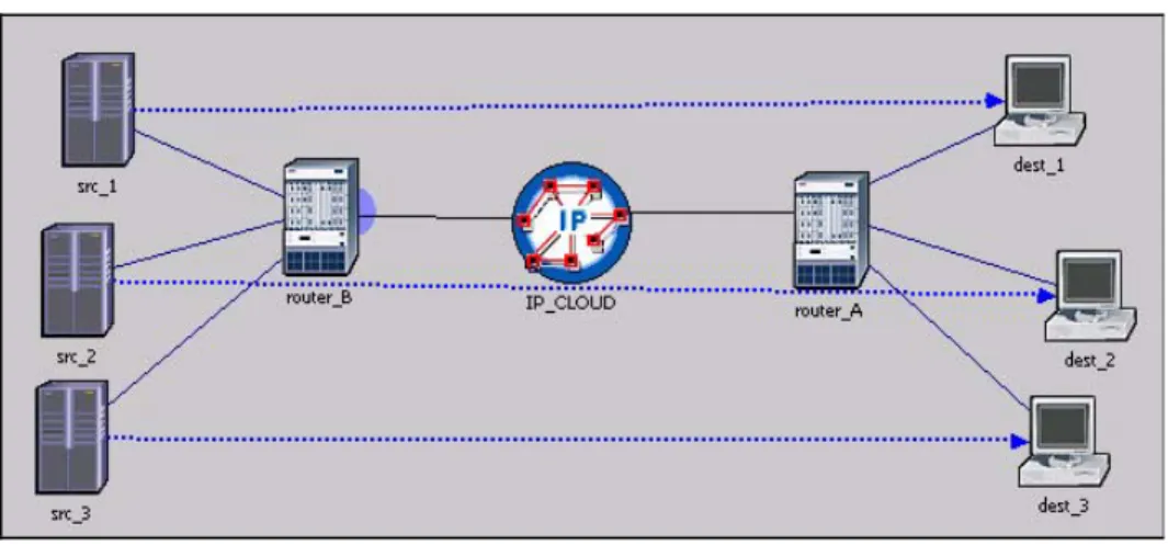
Figure 2-1 Example Network Model
Note—Source nodes (video servers) with different ToS (1,2,3) are shown on the
left-hand side of the Network Model figure; destination nodes on the right.
Router B provide the interface with WFQ.
Simulation with Explicit Traffic
Procedure 2-1 Create a Simple Network with Explicit Traffic 1 Open the project.
1.1 Launch NETWARS, if not already opened.
1.2 From the System Editor’s File menu, choose Open Editor.
1.3 From the Open Editor drop-down menu, select Scenario Builder, and then click OK. The Scenario Builder window displays.
1.4 Select File > Open Project. The Open Project dialog box displays.
1.5 Select the project named 1302_lab1 (or if you want to follow along without actually performing the steps in this procedure, select the project named 1302_lab1_ref instead), and then click Open.
Scenario “Explicit_traffic” appears as the first scenario.
Note—If you do not have access to these files, simply view the screens provided in this user’s guide to follow along with the procedure.
2 Create explicit traffic using IP Traffic Flows.
We will create three traffic flows representing the traffic downloaded by the three classes of clients. In this scenario, all traffic will be modeled as explicit traffic.
2.1 Click the Open Object Palette toolbar button.
2.2 Select the “demands” object palette from the drop-down list.
Figure 2-2 Demands Object Palette
2.3 Click on IP demand “ip_traffic_flow” to define an IP-to-IP background traffic flow.
2.4 Connect the IP demand between src_1 and dest_1 (in the same way you would create a link object).
Figure 2-3 IP Demand Connected
2.5 Right-click on the workspace and select Abort Demand Definition to exit demand operation.
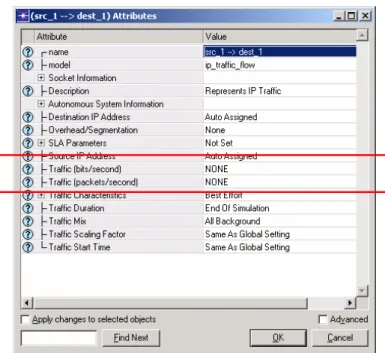
2.6 Right-click on the demand object and select Edit Attributes.
2.7 In the Attributes dialog box, edit the traffic specification for both bits/second and packets/second values as described below.
• Configure the “Traffic (bits/second)” attribute with a value of 6.0 Mbps from 0 to 600 seconds. (The profile name may be different in your case.) The graph is updated when you press Enter after typing the values.
Figure 2-5 Configuring the Traffic (bits/second) Attribute
• Click OK to commit changes.
• Configure the “Traffic (packets/second)” attribute with a value of 500 packets/second from 0 to 600 seconds. (The profile name may be different in your case.) The graph is updated only if you press Enter after typing the values.
Figure 2-6 Configuring the Traffic (packets/second) Attribute • Click OK to commit changes.
Note that the average packet size implied by the configured traffic volumes (6,000,000 bps and 500 pps) is 6,000,0000 bps / 500 pps = 12,000 bits = 1,500 bytes.
2.8 In the Attributes dialog box, set the “Traffic Mix” attribute to “All Explicit”.
2.10Click on the demand object to select it, press Ctrl+C to copy it, and then press
Ctrl+V to paste it in the same direction from src_2 to dest_2 and from src_3 to dest_3 (as shown below.)
Figure 2-7 Copying/Pasting Demand Objects
3 Configure the Type of Service on each demand.
3.1 Select Protocols > IP > Demands > Characterize Traffic Demands.
3.2 Set the Type of Service for the demands originating from WFQ_net.src_1, WFQ_net.src_2, and WFQ_net.src3 to “Background (1)”, “Standard (2)” and “Excellent (3),” respectively.
Figure 2-8 IP Traffic Flow Characterization dialog box
3.3 Click OK.
4 Configure the packet size and packet inter-arrival time distributions.
Next we will configure additional traffic generation parameters, such as statistical distributions used for packet sizes and packet inter-arrival times. Note that these can be configured either individually for each demand, under the “Traffic
Characteristic” attribute, or globally for all the demands using the Background Traffic Config utility. We will use the latter approach in this lab and configure the distributions by modifying the global settings.
4.1 Right-click on the “bkg_config” node and select Edit Attributes.
4.3 Set the “Packet Size Variability” to “constant”.
Figure 2-9 Node’s Attributes dialog box
Note that the average values for both distributions are already determined by the settings in the traffic profile and therefore appear as “Auto_Calculated”. The traffic volume of 500 packets/second in the profile translates into an average packet inter-arrival time of 0.002 seconds. The average packet size is also already determined to be 1,500 bytes.
4.4 Click OK to commit changes.
5 Choose statistics.
We will monitor the queuing delay statistics for each service class on the outgoing interface of “router_B”. This interface is the access interface to the core network and has WFQ scheduling enabled to provide QoS treatment to different service classes. We will also collect the packet end-to-end delay statistics for all the traffic flows.
5.1 Right-click anywhere in the project editor and select Choose Individual DES Statistics.
5.2 Expand “Demand Statistics” by clicking on the (+) next to it, and select the “Packet ETE Delay (sec)” statistic.
5.3 Expand “Node Statistics” by clicking on the (+) next to it, and select the “IP Interface / Queuing Delay (sec)” statistic.
Figure 2-11 Selecting the IP Interface / Queuing Delay (sec) Statistic
5.4 Click OK.
6 Run the simulation.
6.1 Click the Configure/Run Simulation toolbar button. The simulation is set to run for 10 minutes.
6.2 Click Run to start the simulation. (The simulation runs for about 3 minutes.)
Figure 2-12 Simulation Sequence dialog box
6.3 Close the Simulation Sequence dialog box after the simulation runs.
7.1 Right-click on the “router_B ↔ IP_CLOUD” link, and select View Results.
7.2 Expand the “point-to-point” group and select the “throughput (packets/sec) Å” and “throughput (bits/sec) Å” statistics. Click Show.
Figure 2-13 Selecting Throughput Statistics to Show
The graph shows that the total traffic entering the IP cloud is 18 Mbps at the rate of 1500 packets per second (pps) – remember each of the three flows is sending traffic at 6 Mps and 500 pps.
Figure 2-14 Throughput Results Graph
7.4 Right-click on “router_B”, and select View Results.
Figure 2-15 View Results dialog box
7.5 Expand the “IP Interface” group, and select the statistics below in the following order:
• “WFQ Queuing Delay (sec) IF10 Q3”
• “WFQ Queuing Delay (sec) IF10 Q2”
• “WFQ Queuing Delay (sec) IF10 Q1”
7.6 Change the display mode from “Statistics Stacked” to “Overlaid Statistics”.
7.7 Change the “As Is” filter to “average”.
7.8 Click Show.
As expected, the queues with higher priority (ToS) exhibit smaller queuing delays at the access router “router_B”.
7.9 Click Close to close the View Results dialog box.
7.10Right-click on the demand going from “src_2” to “dest_2”, and select View Results.
7.11Select the “Packet ETE Delay (sec)” statistic, and click Show.
Figure 2-17 Showing the Packet ETE Delay (sec) Statistic Graph
The graph shows that the packet end-to-end delay for the “src_2Ædest_2” demand is about 0.0019 seconds.
End of Procedure 2-1
Simulation with Background Traffic
In the following scenario, we replace the explicit traffic with purely background
traffic, run the simulation, and compare the results and the simulation speed.
Procedure 2-2 Configure Demands with Background Traffic 1 Replace explicit traffic with background traffic.
1.1 Switch to the “Background_traffic” scenario (select Scenario > Switch to Scenario > Background_traffic).
1.2 Right-click on the demand going from “src_1” to “dest_1” and choose Select Similar Demands. Note that the other two demands were also selected.
1.4 Change the “Traffic Mix” attribute to “All Background”.
Figure 2-18 Changing the Traffic Mix Attribute
1.5 Check the Apply changes to selected objects checkbox, and click OK.
2 Run the simulation.
2.1 Click the Configure/Run Simulation toolbar button. The simulation is set to run for 10 minutes.
2.2 Click Run to start the simulation. (The simulation runs for about 10 seconds.)
2.3 Close the Simulation Sequence dialog box after the simulation runs.
3 Compare results with those of the previous scenario (with explicit traffic).
3.1 Click the Hide/Show Graph Panels button.
3.2 Load the panels with latest results by selecting DES > Panel Operations > Panel Templates > Load with Latest Results.
The first graph panel displays the queuing delays for various queues at the access router_B obtained in this scenario.
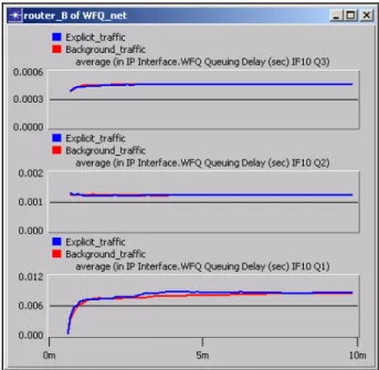
Figure 2-19 Showing Queuing Delays Graph
The second panel compares the individual queuing delays between the two scenarios. Observe that queuing delays for all the queues in both scenarios (explicit and background) are similar.
Figure 2-20 Comparing Queuing Delays
Note that using purely background traffic we were able to significantly reduce the simulation time (from 3 minutes to 10 seconds) and still obtain accurate result for the local queuing delays.
4 Compare end-to-end delay statistics.
4.1 Right-click on the demand going from “src_2” to “dest_2”and select View Results.
Note that the “Packet ETE Delay (sec)” statistic is shaded out and cannot be selected. The delay effects of the background traffic load are simulated only locally on each traffic element (node or link). Because of this, the purely background traffic mode does not provide for end-to-end delays.
Figure 2-21 Inaccessible Packet ETE Delay (sec) Statistic
In the next scenario, we will see how we can overcome this shortcoming by using hybrid traffic (mixture of background and explicit traffic).
End of Procedure 2-2
Simulation with Hybrid Traffic
In the next scenario, we configure the demands to use a mixture of explicit traffic
(1%) and background traffic (99%). This way we can obtain end-to-end statistics
and still achieve significant simulation speedup (compared to the purely explicit
traffic scenario).
Note that the explicit traffic is only a small fraction of the total traffic. This is the
recommended configuration. For flows with large traffic volumes, very small
fractions, such as 0.01% or 0.1% explicit, should be used. Configurations such
as 30% explicit + 70% background traffic do not result in significant simulation
speedup and should be avoided.
Procedure 2-3 Configure Demands with Hybrid Traffic 1 Replace background traffic with hybrid traffic.
1.1 Switch to the “Hybrid_traffic” scenario (select Scenario > Switch to Scenario > Hybrid_traffic).
1.2 Right-click on the demand going from “src_1” to “dest_1” and choose Select Similar Demands. Note that the other two demands were also selected.
1.4 Change the “Traffic Mix” attribute to “1.0 % Explicit”.
Figure 2-22 Changing the Traffic Mix Attribute
1.5 Check the Apply changes to selected objects checkbox, and click OK.
2 Run the simulation.
2.1 Click the Configure/Run Simulation toolbar button. The simulation is set to run for 10 minutes.
2.2 Click Run to start the simulation. (The simulation runs for about 15 seconds.)
2.3 Close the Simulation Sequence dialog box after the simulation runs.
3 Compare results with those of the other scenarios.
3.1 Click the Hide/Show Graph Panels button.
3.2 Load the panels with latest results by selecting DES > Panel Operations > Panel Templates > Load with Latest Results.
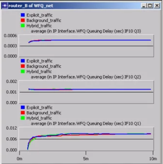
The first panel compares the queuing delays between the three scenarios. The queuing delays obtained in this scenario using hybrid traffic match with those from previous scenarios.
Figure 2-23 Comparing Queuing Delays
The second graph panel compares the packet end-to-end delays for the three traffic demands obtained using explicit traffic and hybrid traffic (no ETE delays were available in the purely background traffic scenario). The results obtained using the two traffic types match closely.
Figure 2-24 Comparing Packet ETE Delay (sec) Statistics End of Procedure 2-3
Conclusion
In this section, we have demonstrated how using background and/or hybrid traffic can help reduce the simulation time without significant losses in the accuracy of the results.
Using Hybrid Simulation to Model New Application Performance
In this section, we study the performance of a new application deployed in a
Wide Area Network (WAN). The preexisting baseline traffic in the network is
modeled using link loads. The new application is recreated from an actual traffic
trace and converted into OPNET application traffic using ACE.
In the first scenario, we deploy one instance of the new application in an empty
network (without the baseline traffic). The application user is modeled using
discrete traffic. We assess the application performance and verify whether it
conforms to the Service Level Agreement (SLA) requiring that the application
response time is below 30 seconds. Next we add the baseline traffic (modeled
as link loads) and observe its impact on the application response time. After
that, we use ACE and deploy additional application users, modeled not as
discrete traffic, but using background traffic flows. We monitor the application
response time and apply QoS to improve the application performance.
Procedure 2-4 Use Hybrid Simulation to Model Application Performance 1 Examine the new application trace in ACE.
1.1 Launch NETWARS, if not already opened.
1.2 From the System Editor’s File menu, choose Open Editor.
1.3 From the Open Editor drop-down menu, select ACE, and then click OK. The ACE Import WIzard displays the ACE Import: Choose Capture File(s) dialog box.
1.4 Click Add Capture File. The Select Capture File for Import dialog box displays.
1.5 In the Select Capture File for Import dialog box, select the file named cwd_local, and then click Open. The selected file name displays in the
Capture Filecolumnof the ACE Import: Choose Capture File(s) dialog box.
Note—If you do not have access to this file, simply view the screens provided in this user’s guide to follow along with the procedure.
1.6 Continue to follow the ACE Import Wizard screens as they are presented to you until the Treeview window displays.
Figure 2-25 Treeview window
1.7 Click the Data Exchange Chart button.
Figure 2-26 Data Exchange Chart
The Data Exchange Chart shows the application traffic patterns between the different tiers. Note that there are 3 tiers in this application: web_client, web_server and database_server. The horizontal lines represent the tiers - the topmost line corresponds to the web_client, the middle line to the web_server, and the bottom line represents the database_server. The color arrows connecting the three horizontal lines represent individual packet exchanges between the tiers. The horizontal axis visualizes the time of the transaction in seconds. The application is a typical database query. Initially the web_client contacts the web_server with a request and the two exchange
several packets. After that the bulk of the traffic exchange is between the web_server and the data_server. At the end of the application the web_server sends replies to the web_client. Note that the duration of the whole application is about 8.1 seconds.
1.8 Click Close to close the Data Exchange Chart.
1.9 Close the ACE editor.
2 Deploy one application user running discrete traffic.
Configure the network to use one instance of the ACE application. The following nodes will be used as the application tiers: web_client Æ San Diego, web_server Æ Los Angeles, and database_server Æ Houston.
2.1 Launch NETWARS, if not already opened.
2.2 From the System Editor’s File menu, choose Open Editor.
2.3 From the Open Editor drop-down menu, select Scenario Builder, and then click OK. The Scenario Builder window displays.
2.4 Select File > Open Project. The Open Project dialog box displays.
2.5 Select the project named 1302_lab2 (or if you want to follow along without actually performing the steps in this procedure, select the project named 1302_lab2_ref instead), and then click Open.
Scenario “app_user_only” appears as the first scenario.
Note—If you do not have access to these files, simply view the screens provided in this user’s guide to follow along with the procedure.
2.6 Click Protocols > Applications > Deploy ACE Application on Existing Network > as Discrete Traffic. The Configure ACE Application dialog box displays.
2.7 In the Configure ACE Application dialog box:
• Set the application “Name” to “my_app”
• Set the “Repeat” to “20 times per hour”
• Click the Add Task button and select the “cwd_local.atc.m” ACE trace file.
Figure 2-28 Configure ACE Application dialog box 2.8 Click Next.
In the next step we will assign application tier functionality to existing nodes in the network.
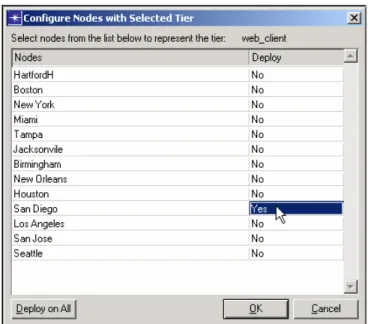
2.9 Click “Select Nodes” for the “web_client” tier.
2.10Select “San Diego” from the node list by clicking on the “Deploy” column value.
2.11Click OK.
Figure 2-30 Configure Nodes with Selected Tier dialog box
2.12In a similar fashion, choose “Los_Angeles” to function as the web_server and “Houston” to represent the database_server.
2.13Click Deploy.
3 Run the simulation and view results.
3.1 Click the Configure/Run Simulation toolbar button. The simulation is set to run for 1 hour.
3.2 Click Run to start the simulation.
3.3 Close the Simulation Sequence dialog box after the simulation runs.
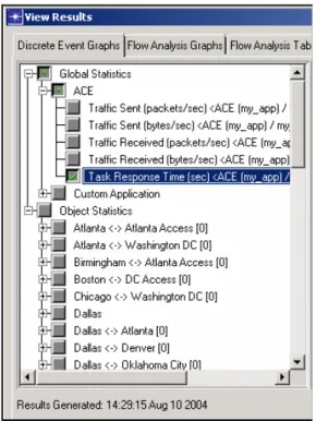
3.5 In the View Results dialog box, expand “Global Statistics / ACE” and select the “Task Response Time (sec)” statistics.
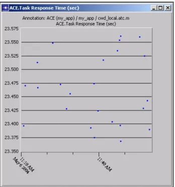
Figure 2-31 Selecting the Task Response Time (sec) Statistic 3.6 Click Show.
Note the application response time varies around 23.2 seconds. This conforms to the 30 second limit required by the SLA.
3.7 In the View Results dialog box, change the display filter from “As Is” to “average”.
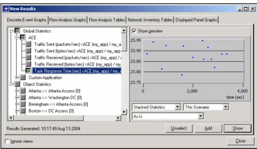
Figure 2-33 View Results dialog box 3.8 Click Show.
The graph shows the average response time for the new application.
Note—Remember that the duration of the application in the ACE editor was about 8.1 seconds. However, the application response time statistics now show that it takes about 23.2 seconds to complete the applications. Why the difference? The application trace was captured on a local network and all the tiers were part of the same LAN. In this scenario the application is deployed in a WAN and the
application tiers are placed in different geographical locations (San Diego, Los Angeles, Houston). This causes addition latency in the communication between the tiers, and as a result of this the application response time increases.
4 Include pre-existing baseline traffic.
In the next scenario, we add the baseline traffic (modeled as link loads) and observe its impact on the new application.
4.1 Switch to the “app_user_and_linkloads” scenario (select Scenario > Switch to Scenario > app_user_and_linkloads).
This scenario already includes the application traffic we configured in the previous scenario. In addition there are background loads configured on the links that represent the pre-exiting baseline traffic (link loads can be
configured manually or imported from a variety of traffic management tools).
4.2 To view an example traffic load profile, right-click on the Salt Lake City ↔
Dallas link and select Edit Attributes.
4.3 Click the “Background Load” attribute and select Edit....
Figure 2-35 Link Attributes dialog box
4.4 Click the “Intensity (bps) [Salt Lake City Æ Dallas]” attribute and select Edit....
The profile captures the WAN link traffic during business hours on May 6 (from 8am to 6pm). Note the green vertical line in the profile whose position indicates the current network time. The current network time can be
configured in the Time Controller tool (invoked by Ctrl+Alt+T). In this scenario the current network time has been pre-configured to 11 am, so that the 1-hour simulation that we will run includes the busiest period of the workday (from 11 am to 12 pm).
Figure 2-37 Profile dialog box
4.5 Click Cancel until you have closed all the Attribute dialog boxes.
5 Run the simulation and view the results.
5.1 Click the Configure/Run Simulation toolbar button.
5.2 Click Run to start the simulation.
5.3 Close the Simulation Sequence dialog box after the simulation runs.
5.5 Expand “Global Statistics / ACE” and select the “Task Response Time (sec)” statistics.
Figure 2-38 View Results dialog box 5.6 Click Show.
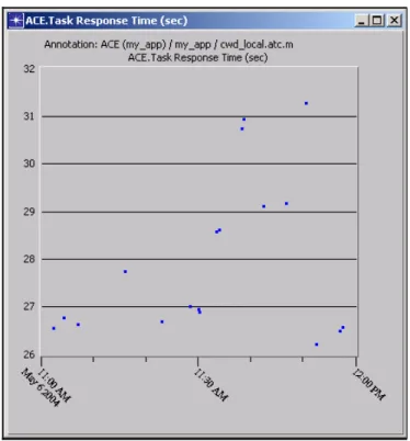
Compared to the previous scenario, as a result of including the baseline traffic load, the application response time increased by about 0.7 seconds to 23.9 seconds. The response time is still, however, well below the SLA limit (30 seconds).
Figure 2-39 Task Response Time Statistics
Note—The above result indicates that under current traffic conditions the network has sufficient spare capacity to support one new application within the SLA limits. Will the network capacity be enough to support thousands of new users? Continue on to the next scenario.
6 Deploy additional application users modeled as traffic flows.
In the following scenario, we configure an additional 1,690 application users in the network. This time, however, the users will not be modeled using discrete traffic, but rather as background traffic flows. We could model all the new users as explicit traffic, but that might result in a long simulation time. To get a quick answer, we use mixed traffic and hybrid simulation.
6.1 Select Scenario > Duplicate Scenario.
6.2 Name the new scenario “add_app_users_as_flows”.
6.3 Select Protocols > Applications > Deploy ACE Application on Existing Network > as Traffic Flows.
6.4 In the ACE Traffic Import: Specify Tasks dialog box under “Tasks”, click on “Click here to add new task”, select the “cwd_local” trace file, and then click
Next.
Figure 2-40 ACE Traffic Import: Specify Tasks dialog box
6.5 Assign nodes for each of the application tiers. Click on “ACE Tier web_client <initiating_tier>” to select it.
Next, assign all thirteen end-nodes in the network to support one hundred and thirty web_clients each (1,690 users total).
6.6 Go to the project editor, right-click on Seattle, and choose Select Similar Nodes.
6.7 Return to the ACE Traffic Import: Assign Nodes dialog box, and click Assign Selected Nodes.
6.8 In the ACE Traffic Import: Configure Initiating Node dialog box:
• Set the “Number of users” to “130”.
• Set “Repetitions per user per hour” to “20”.
• Check the Apply to remaining nodes (12) checkbox.
Figure 2-42 ACE Traffic Import: Configure Initiating Node dialog box
6.9 Click OK.
Note that the 13 selected nodes were added to the web_client list.
6.10Next we will assign five nodes to support the web_server functionality. Click on “ACE Tier web_server” to select it.
6.11Go to the project editor. Click in the workspace to unselect the previously selected nodes. While holding the Shift key, click on the following five nodes to select them: Seattle, Los Angeles, Houston, Miami, New York.
6.12Return to the ACE Traffic Import: Assign Nodes dialog box, and click Assign Selected Nodes.
The five nodes should now appear listed under the web_server.
Figure 2-44 Node Assignments (web_server) List
6.13Finally, click on the “ACE Tier database_server” to select it. Select Houston in the project editor, and click Assign Selected Nodes. Houston will be added to the list.
Figure 2-45 Node Assignments (database_server) List
6.14Click Finish. Observe the purple traffic demands added to the network to represent the traffic generated by the new application users.
7 Run the simulation and view the results.
7.1 Click the Configure/Run Simulation toolbar button.
7.2 Click Run to start the simulation.
7.3 Close the Simulation Sequence dialog box after the simulation runs.
7.4 Click DES > Results > View Statistics.
7.5 Expand “Global Statistics / ACE” and select the “Task Response Time (sec)” statistics. Click Show.
Figure 2-47 Task Response Time Statistics
Note that the application response time increased dramatically and some of the values are above the 30-second Service Level Agreement limit.
7.6 To find the reason for this increase, select DES > Results > Find Top Statistics. Expand the “Link Statistics / point-to-point” group and select “utilization”. Click Find Top Statistics.
Figure 2-48 Select Statistic for Top Results dialog box
7.7 Observe that as a result of adding new ACE application users, several links in the network become over 97% utilized. The link utilization for the “Dallas Access ↔ Dallas” link reaches 99.4%.
Figure 2-49 Top Objects Point-to-Point Utilization dialog box
7.8 Close the above window showing link utilizations.
The above results indicate that the current network bandwidth will not be enough to support the new application on top of the pre-existing traffic. This problem can be solved either by increasing the network capacity or applying some QoS techniques to prioritize the critical traffic. We will try out the latter approach and apply Quality of Service in the next scenario.
End of Procedure 2-4
Implementing QoS in the Network and Prioritizing Application Traffic
In the following scenario, we apply Weighted Fair Queuing (WFQ) to all the
routers in the network. We will configure a high-priority Type of Service on the
ACE application traffic (both discrete and flow based) and thus give it
preferential treatment over the pre-existing traffic (link loads).
Procedure 2-5 Implement QoS in the Network and Prioritize Traffic 1 Choose Scenario > Duplicate Scenario.
2 Name the new scenario “with_qos”.
3 Apply WFQ on all the interfaces in the network.
3.1 Select Protocols > IP > QoS > Configure QoS.
3.2 In the QoS Configuration dialog box:
• Set the “QoS Scheme” to “WFQ (Class Based)”.
• Set the “Qos Profile” to “ToS Based”.
• Uncheck the Visualize QoS configuration checkbox.
Figure 2-50 QoS Configuration dialog box • Click OK.
4 Set the Type of Service on all the traffic representing the new application (i.e. both the discrete traffic and the flows) to give it a preferential treatment over the baseline traffic.
4.1 To set the Type of Service on the traffic flows, right-click on any demand in the network and choose Select Similar Demands.
4.2 Right-click on the same demand and select Edit Attributes.
4.3 Expand the “Traffic Characteristics” attribute group by clicking on the (+) sign next to it. Set the “Type of Service” attribute to “Interactive Multimedia (5)”.
Figure 2-51 Attributes dialog box
4.4 Check the Apply changes to selected objects check box, and click OK.
5 Change the Type of Service on the discrete application traffic.
5.1 Right-click on the “Applic Config” utility node and select Edit Attributes.
5.2 Click on the “Application Definitions” value and select Edit.
5.3 Edit the Description for “my_app”.
Figure 2-53 Application Definitions Table
5.4 Edit the Value for “Custom”.
Figure 2-54 Descriptions Table
6 Change the “Type of Service” attribute to “Interactive Multimedia (5)”.
Figure 2-55 Custom Table
6.1 Click OK as often as needed to close all the open dialog boxes.
7 Run the simulation and view the results.
7.1 Click the Configure/Run Simulation toolbar button.
7.2 Click Run to start the simulation.
7.3 Close the Simulation Sequence dialog box after the simulation runs.
7.5 Expand “Global Statistics / ACE” and select the “Task Response Time (sec)” statistics. Click Show.
Figure 2-56 Task Response Time Statistic
We can see that applying QoS and prioritizing the new application helped achieve the goal. The application response time is about 23.5 seconds, which is below the 30-second SLA limit.
3
Importing IP and Layer 2 Networks with MVI
Introduction
The Multi-Vendor Import (MVI) module gives you a practical way to import
topology and traffic data from the production network environment. The Device
Configuration Import (DCI) feature of the MVI module lets you automatically
create high-fidelity network models by importing router and switch configuration
data.
This chapter shows you how to use the DCI features to import from switch,
router, and security appliance configuration files. DCI’s current platform support
includes Cisco IOS, Cisco CatOS, Cisco PIX, and Juniper JunOS devices.
Note—The following examples were presented at OPNETWORK 2004 in
Session 1617, Importing IP and Layer 2 Networks with MVI. If you do not have
access to the files that these procedures use, you can still follow along using the
sample screens provided in this user’s guide.
Import an Example Network
A set of router configuration files is provided for an enterprise scale network. In
this example, we will import the device configuration files to create a network
model and explore it using available visualization features.
Procedure 3-1 Import Device Configuration Files 1 Launch NETWARS, if not already opened.
2 From the System Editor’s File menu, choose Open Editor.
3 From the Open Editor drop-down menu, choose Scenario Builder, and then click
OK.
4 Create a new project.
4.1 Choose File > New Project, and click OK.
4.2 Name the project Session_1617.
4.3 Name the phase Lab_1, and click OK.
4.4 Choose Topology > Import> Device Configuration Files... The Import Device Configurationsdialog box opens.
5 Specify folders for device configuration files [we will look into in detail on vendor types later in the procedure].
5.1 Select the checkbox for Cisco (IOS, CatOS, PIX).
5.2 Click the Browsebutton for Cisco (IOS, CatOS, PIX), and select the folder:
C:\Netwars\User_Data\Projects\Session_1617\Lab_1\Cisco 5.3 Select the checkbox for Juniper (JunOS).
5.4 Click the Browsebutton for Juniper (JunOS) and select the folder:
C:\Netwars\User_Data\Projects\Session_1617\Lab_1\Juniper 5.5 Specify import options [we will look into in detail on import options later in the
procedure].
5.6 Select the checkbox for Generate import log.
5.7 Select the checkbox for Create PVCs.
5.8 Leave other options unchecked.
6 Import.
6.1 Make sure your settings are as shown below:
Figure 3-1 Import Device Configurations dialog box 6.2 Click Import.
7 The Open Import Assistant dialog box displays. It reports that the network has unnumbered interfaces and connected interfaces with data rates unspecified. For now, click Cancelto close the dialog box; you will come back to this in a later procedure.
8 Save the project.
The imported network should look as follows:
Figure 3-2 Sample Network
The import process is now complete.
End of Procedure 3-1
Exploring the OPNET Network Model
In this section you will explore different parts of the imported network model
using built-in visualization tools.
Procedure 3-2 Explore the OPNET Network Model 1 Zoom to the core of the network in the network editor by:
1.2 Drag the cursor to create a box around the area of interest.
Figure 3-3 Zoom In
Note—If you want to zoom to another area, you can come back to the original view by clicking the Zoom Out toolbar button.
2 Observe that the different types of links are shown in different colors.
Figure 3-4 Link Types in Color
PVCs are shown using dashed lines in the same color as the corresponding link
A T M – g re e n
S e ria l – b la c k
E th e rn e t – r e d
3 Hide all logical connections. Right-click on a demand object, and select Hide Similar Demands.
4 Click the Zoom Out button to go back to the top-level view, and choose View > Show Network Browser(Ctrl + B).
Figure 3-5 Network Browser
5 View link tool tip:
5.1 In the network browser, choose Links from the top drop-down list. The network browser shows the list of links in the network ordered alphabetically.
5.2 In the browser, choose the link Albany / Serial0/0 <-> 172_16_249_12/30(+) .
5.3 The link between Albany and the FR cloud gets selected in the project editor. Point your mouse at this link for a few seconds.
5.4 If you can’t find the link in the network, double-click on it for the editor to auto-zoom to that part of the network.
Link tool tip displays link type; node, interface, and IP address; and data rate.
Figure 3-6 Link Tool Tip
6 In the network browser, change back to Nodes from the top drop-down list; Select the router Albany, observe that the node is selected on the network browser at the top left corner of the network.
7 Choose View > Show Network Browseragainto close the network browser.
8 View command mappings for interface FastEthernet0/0.
9 Right-click on router Albany, and select Edit Attributes.
11 Go to the Interface Information attributeunder IP Routing Parameters. Each physical interface of the router is mapped to a single row under this attribute.
Figure 3-7 Attributes dialog box
Figure 3-8 Interface Information Attribute
12 Observe the values set on the attributes IP Address and Subnet Mask for interface FastEthernet0/0. They are 172.16.114.1 and 255.255.255.0 respectively. These are the same values as you noticed before in the configuration file.
13 Click Cancelto close the dialog box that shows interface information.
14 Click Cancelto close the dialog box that shows attributes for node Albany.
15 View subinterface information.
16 Right-click on router Albany again, and select View Device Configuration Source Data.
17 Scroll down to see the subinterfaces configured for the device.
Figure 3-9 Device Subinterfaces
18 Interface Serial0/0 has subinterfaces Serial0/0.101, Serial0/0.102. Notice on line 53 that Serial0/0.101 has an OSPF cost set to 500.
19 Close the window that shows the configuration file.
20 Right-click on router Albany and select Edit Attributes.
21 Expand the attribute group IP Routing Protocols.
22 Go to the Interface Information attribute under OSPF Parameters.
23 Choose Subinterface Information for interface Serial0/0. Each subinterface of the physical interface is mapped to a single row under OSPF Parameters > Interface Information > Subinterface Information.
24 You can notice subinterfaces Serial0/0.101, Serial0/0.102, etc., configured here. Note that the Cost field of interface Serial0/0.101 is set to 500, as noted in the configuration file.
Figure 3-10 Attributes dialog box
Figure 3-11 Interface Information Attribute
Figure 3-12 Subinterface Information Attribute
25 Click Cancelto close the dialog box that shows subinterface information.
26 Click Cancelto close the dialog box that shows interface information.
27 Click Cancelto close the dialog box that shows attributes for node Albany.
Procedure 3-3 View Skipped Commands 1 View log messages:
1.1 Right-click on router Albany and select View Detailed Import Log. The following dialog box displays.
Figure 3-13 Log Browser Showing Skipped Commands for Albany
Skipped commands are shown according to their class and subclass.
1.2 Expand the tree-view in the left to see the various categories of skipped commands.
1.3 Choose subclass FastEthernet0/0, under Interface class in the tree-view to view the skipped commands for this particular interface. These are
commands that are currently not supported by DCI.
Figure 3-14 Log Browser Showing Skipped Commands for FastEthernet0/0 1.4 Click Close to close the dialog box that shows log messages.
Procedure 3-4 Visualize the Network Model
1 Choose View > Visualize Protocol Configuration > IP Routing Domains
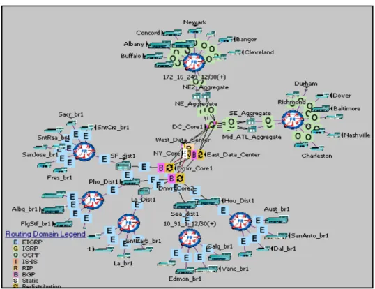
(Ctrl+Shift+V) to visualize the routing domains in the network. The network’s routing domains display as follows.
Figure 3-15 Sample Network’s Routing Domains
2 Scale the icons in the network.
2.1 Choose View > Visualize Protocol Configuration > Clear Visualization to clear routing domain visualization.
2.2 Left-click in an empty space in the project editor to deselect all objects.
2.3 Choose View > Layout > Scale Selected Icons.
Figure 3-16 Scale All Icons dialog box 2.4 Set Scale factor value to 25.
Notice, the icons become smaller; in many cases where you have a very large topology, scaling can help to get a better view of the network and its topology.
2.5 Click Cancel to close the Scale All Icons dialog box.
3 Choose File > Save Project to save the project.
End of Procedure 3-4
Conclusions
The Multi Vendor Import module (MVI) allows you to import network topology
using device configuration files. Using the “Import Logging” feature, you can
view the commands that the Device Configuration Import (DCI) does not use
during the import.
The network browser is useful for navigating through the network. NETWARS
provides several visualization features that make it easy to understand the
network topology and configuration.
Importing from device configuration files provides the ability to build a network
model, however all the relevant info is not contained in the configuration files.
In the following procedure, you will learn how to provide supplemental
information to deal with these inadequacies.
Using the Model Assistant
The device configuration files obtained from a network may not always contain
all of the necessary information to model the network accurately. In this section,
we will import a new set of configuration files with missing information and see
how we can provide additional information during and after the import process
using the Model Assistant.
Procedure 3-5 Import the Configuration Files 1 Launch NETWARS, if not already opened.
2 From the System Editor’s File menu, choose Open Editor.
3 From the Open Editor drop-down menu, choose Scenario Builder, and then click
OK.
4 Select File > Open Project. The Open Project dialog box displays.
5 In the Open Project dialog box, select the project file named Session_1617, and then click Open.
Note—If you do not have access to this file, simply view the screens provided in this user’s guide to follow along with the procedure.
6 Create a new scenario: Choose Scenario > New Scenario, name the scenario Lab_2, and click OK.
7 Choose Topology > Import> Device Configuration Files... The Import Device Configurationsdialog box opens.
8 Specify import settings:
Note—The Import Device Configurations dialog box retains its settings from the previous import; the following steps will direct you based on the retained settings in the dialog box from the previous procedures in this chapter.
8.1 Keep the checkbox for Cisco (IOS, CatOS, PIX)checked.
8.2 Click the Browse button for Cisco Router IOS and select the folder:
C:\Netwars\User_Data\Projects\Session_1617\Lab_2\Cisco_R outers
8.3 Keep the checkbox for Juniper (JunOS)checked.
8.4 Click the Browse button for Juniper JunOS and select the folder:
C:\Netwars\User_Data\Projects\Session_1617\Lab_2\Juniper _Routers
8.5 Toggle off the import option Generate Import Log.
8.6 Keep the Create PVCs option checked.
8.7 Check that the dialog box appears as follows:
Figure 3-17 Import Device Configurations dialog box
9 Import:
9.2 After import of the network model, the following dialog box displays:
Figure 3-18 Open Import Assistant
The Open Import Assistant dialog box displays automatically when the import process detects that all of the necessary information cannot be found within the device configuration files. The Import Assistant requests, but does not require, that you provide supplemental information.
9.3 Click Open. The following dialog box displays:
Figure 3-19 Import Assistant dialog box
End of Procedure 3-5
Procedure 3-6 Use Import Assistant to Connect Interfaces and Specify Data Rates
1.1 Make sure that the Show pull-down menu is set to Routers with unnumbered interfaces.
1.2 In the interface A pane, click on the (+) sign next to the router icon for
Boston_Bkup_IDC to expand the view of the router to include its name and interfaces.