ISSN 1755-5361
Discussion Paper Series
Designing large value payment systems:
An agent-based approach
Sheri Markose, Amadeo Alentorn, Stephen Millard and
Jing Yang
Note : The Discussion Papers in this series are prepared by members of the Department of Economics, University of Essex, for private circulation to interested readers. They often represent preliminary reports on work in progress and should therefore be neither quoted nor referred to in published work without the written consent of the author.
University of Essex
Department of Economics
Designing large value payment systems:
An agent-based approach
Sheri Markose*, Amadeo Alentorn**, Stephen Millard# and Jing Yang
*
University of Essex, Economics Department
** OMAM and Centre For Computational Finance and Economic Agents (CCFEA)
#
Bank of England, Threadneedle Street, London EC2R 8AH Bank of International Settlements,
E-mail: [email protected]
[email protected] [email protected]
Abstract
The purpose of this paper is to show how agent-based simulations of payment systems can be used to aid central bankers and payment system operators in thinking about the appropriate design of payment settlement systems to minimise risk and increase their efficiency. Banks, which we model as the ‘agents’, are capable of a degree of autonomy with which to respond to payment system rules and adopt a strategy that determines how much collateral to post with the central bank at the start of the day (equivalently how much liquidity to borrow intraday from the central bank) and when to send payment orders to the central processor. An interbank payment system with costly liquidity requires banks to solve an intraday cash management problem, minimising their liquidity and delay costs subject to their beliefs about what the other banks are doing. We use the Erev and Roth (1998) reinforcement learning algorithm for banks to
endogenously determine how much liquidity to post in the interbank liquidity management game.
Keywords: Agent-based simulation; Payment Systems; Liquidity; Systemic Risk
The views expressed are those of the authors and do not necessarily reflect those of the Bank of England or the Bank of International Settlements. The authors are grateful for comments received from seminar participants at the Bank of England, Cass Business School and the University of Essex.
Contents
1 Introduction 3
2 Payment systems in practice 5
3 An agent-based model of a payment system 7
4 An example experiment 12
4.1 Liquidity posted at opening 13
4.2 Liquidity is raised just in time 14
5 Results 14
5.1 Liquidity-delay trade off in RTGS 14
5.2 The impact of operational events in the two systems 16 6 Analysis of Erev- Roth reinforcement learning by banks
to determine optimal liquidity (alpha): Opening Liquidity system
7 Concluding remarks and future work 17
1 Introduction
The purpose of this paper is to show how the methodology of ‘agent-based modelling’ can be used to examine interbank payment systems, defined as ‘a set of instruments, banking procedures and, typically, interbank funds transfer systems that ensure the circulation of money’, (Bank for International Settlements (2003)). The interbank flow of large-value payments increased substantially in the 1980’s and 1990’s as a result of financial innovation, deregulation and globalisation of financial markets. On a daily basis it has been estimated that close to 20% of a country’s GDP typically comes up for settlement in the interbank payment networks of each of the G10 countries.(1) Given that the smooth functioning of payment systems is clearly important for financial stability, the central bank should have an understanding of the risks associated with different systems and seek to minimise these where it can do so in a cost-effective manner. Bank of England (2000) discusses four types of risk in payments systems:
Credit risk: the risk that a bank will not actually meet a payment obligation incurred by it either when the obligation is due or at a later stage
Liquidity risk: the risk that a bank won’t meet an obligation at the time it is due, although it will at some point thereafter (as a result of being ‘short of liquidity’)
Operational risk: the risk that the system breaks down or fails to function and this results in possible financial losses
Legal risk: the risk that unexpected legal decisions or legal uncertainty more generally will leave the system or its members with unforeseen obligations and possible losses
By thinking of the participants – ‘settlement banks’ – in a payment system as our ‘agents’, one can construct a model of a payment system in which the agents adopt strategies that determine how they behave given the ‘instruments and procedures’ in a particular payment system. In particular, such strategies would include rules for much collateral to post with the central bank at the start of the day (equivalently how much liquidity to borrow intraday from the central bank), when to send payment orders to the central processor and what priority to attach to each payment. Simulations of such models can be used to aid central bankers and payment system operators in thinking about the appropriate design of payment systems to minimise these risks.
A number of alternative methodologies have been used to examine these issues. On the more theoretical side, Angelini (1998), Bech and Garratt (2003) and Willison (2005) have used a game-theoretic perspective to understand the differences in incentives for the banks created by different credit and settlement arrangements in interbank payments. McAndrews (2005) refers to this strand of work as being a ‘market microstructure’ approach to payment systems. He argues that different payment system designs are analogous to the different institutional arrangements found in different financial markets. Hence, insights from the study of financial market microstructure can be used to consider the risk and efficiency implications of different payment system designs and that advances in the analysis of real-time data can be used to evaluate these theories.
1 In the United Kingdom, CHAPS processes some £200 billion per day with a transactions volume of about 100,000.
These papers are insightful and give qualitative suggestions on design issues. However, they cannot address the trade-offs between the different risks, and the costs associated with system designs that minimise them, in the quantitative fashion that is needed for a realistic comparison of different ‘real-life’ interbank payment systems. Further, these authors are typically forced to make a number of simplifying assumptions in order to solve their models. Indeed, it is well known that it is difficult to solve a formal model of a network of independent, optimising agents interacting with each other in an environment that is even close to reality. But such assumptions are not always innocuous. For instance, most models assume that banks know in advance what payments are coming in to them over the course of the day; this makes liquidity planning much easier than it ever would be in practice. Finally, we show how an Erev and Roth (1998) type reinforcement learning algorithm can be used for banks to endogenously determine how much liquidity to post in the interbank liquidity management game. However, it is beyond the scope of this paper to show how agent based modelling can be used to see how bank behaviour may evolve over time, particularly in response to the actions of other participants, and how certain ‘conventions’ in payments behaviour arise.
An alternative theoretical approach to examining the trade-off between risk and efficiency in payment systems can be found in Lester et al (2005). These authors adopt a ‘search-theoretic’ approach to modelling payments and develop a model within which they examine the trade-off between cost and risk of deferred net settlement (DNS) and real-time gross settlement (RTGS) payment systems. But their approach is not suitable for examining the behaviour of participants within a payment system since, in their model, payment requests received by banks are assumed to be automatically forwarded to the system; banks have no discretion over this.
Another popular methodology is that of payment system simulations (PSS). Leinonen (2005) brings together a number of papers in this vein, most of which use a simulator developed by the Bank of Finland (BoF PSS for short). In this approach, authors typically use actual data on the arrival of payment requests at the central payments processor and experiment with different
settlement rules, analysing the trade-off between liquidity used and speed in processing payments. The BoF PSS has also been used (for example, in Bedford et al (2005)) to examine the effect of operational events (such as a bank’s IT system crashing leaving it unable to make payments) and bank defaults on the ability of the remaining banks to make payments. Although, this approach is similar to ours, it suffers from the problem that it takes the behaviour of the participating banks as given. In particular, it cannot deal with the strategic decision of the banks to delay payments or that of how much liquidity to post in the first place. In addition, it assumes that bank behaviour and network interconnections in the system remain unchanged across experiments; we might expect both to change given different payment system designs.
In agent-based simulations, we can simulate bank behaviour by starting the banks off with simple rules and allowing them to revise these rules as they deliver outcomes that are better or worse in terms of their objective functions. Given this, we can watch the evolution of payments behaviour over time in different systems by using real payments data as input. Alternatively, we can run ‘stochastic simulations’ that would enable the experimenter to vary the statistical properties of the interbank system in terms of the size, arrival times of payment requests and distribution of the payment flows in the interbank system. For instance, one can compare payment systems we see
in practice with the perfectly symmetrical (identical banks making the same number of equal-sized payments to one other) systems that form the basis of most theoretical models of payments, examining, for example, the implications for liquidity requirements and systemic risk in each system.
As an example of this approach, we conduct a set of experiments that throw some light on the relative merits of two ‘vanilla’ variants of an RTGS system: one in which banks generate all the liquidity they need to use the system by posting collateral with the Central Bank at the beginning of the day – opening liquidity (OL) – and one in which they generate liquidity, by borrowing from the Central Bank, as and when they need it – just in time (JIT). In the JIT system banks weigh up the costs of delaying a payment against the interest they would need to pay on a loan from the central bank in order to determine when liquidity is used. We compare the performance of these systems in terms of a liquidity-delay trade off.
The rest of the paper is organized as follows. In Section 2 we discuss the main issues in payment system design. In Section3 we set out the computational modelling framework. In Sections 4 and 5 the results of our example experiment are reported. Section 6 briefly discusses how the Erev and Roth (1998) reinforcement learning algorithm can be used for banks to endogenously determine how much liquidity to post in the interbank liquidity management game. Section 7 gives the conclusions and discusses future work.
2 Payment Systems in Practice
Historically, interbank payments following the clearing house tradition for paper based IOUs such as cheques have involved central processing with multilateral net settlement at the end of the day. Such end-of-day netting systems were the norm when the process of transmitting payments was expensive and the physicality of the IOUs militated against real-time settlement. But these Deferred Net Settlement (DNS) systems can generate large intraday credit exposures.
Notification by payer banks of payment requests to customers of payee banks, result in the latter processing payments, granting de facto credit extensions to the initiating/payer banks until final settlement occurs at the end of day. Further, in a DNS system, as banks treat the promised inflows with a substantial degree of finality they typically make no explicit arrangements for any liquidity in excess of the end of day multilateral netted amount.
As the size and volume of payments grew larger, the corresponding increase of risk of non-settlement by payer banks in DNS led to the introduction of Real Time Gross Settlement (RTGS) systems in the 1990’s by all EU and G10 countries (with the exception of Canada). In a RTGS system all payment requests arriving at the central processor are processed individually, with immediacy and finality using the balance in a bank’s settlement account. Those payments that do not satisfy the criteria set out by the rules are returned to the sender unpaid.(2) While settlement risk can, in principle, be eliminated completely by RTGS, such systems require large quantities of intraday liquidity. As an alternative, banks can use payment inflows to finance subsequent
2 For a fuller discussion of the different variants of the RTGS in practice, see McAndrews and Trundle (2001).
outflows, strategically delaying the settlement of payments requested in anticipation of offset. Such delaying tactics, which result in hidden queues of unsettled payments, though individually rational, can result in ‘bad’ equilibrium outcomes, compromising the efficiency of the system (see, for example, Angelini, 1998, or Bech and Garratt, 2003).
The relative advantages of DNS and RTGS systems have led to the recent development of hybrid systems that combine the bilateral or multilateral netting features of DNS with RTGS to reduce liquidity requirements and to rid RTGS of the potential for free riding. The maximum benefits from a hybrid system arise when the system operates at the lowest possible level of liquidity, all payments are cleared in full at the time they are made, and all payments are made early in the day. (See Willison (2005) for a discussion of this.)
The intraday liquidity needed in a payment system is a non-trivial function of the random arrival times of payments as well as the size and distribution of payments among banks. For a DNS system, if every bank is assumed to owe every other bank the same value of payments, with multilateral or bilateral netting done at end of day, the liquidity needed will be zero. Given the lack of symmetry in the value (and volume) of real world interbank payment flows, the end of day multilateral netted amount is positive and typically about 2.5% - 3 % of the total value of payments. This amount, calculated by a multilateral netting algorithm on the end of day liability matrix of the interbank settlement system, is generally referred to as the ‘lower bound’ level of liquidity needed by a payment system. The ‘upper bound’ level of liquidity needed by a payment system, on the other hand, is equal to the amount of liquidity that banks require so that all payment requests are settled immediately at the time they are requested with no payments being queued. This value is typically far less than the total value of payments processed in the system and reflects the speed with which liquidity is recycled. If banks post less than their upper bound level of liquidity, the possibility arises of payment gridlock. Bech and Soramäki (2002) define a gridlock as one where the (possibly hidden) queues of payment requests of banks can be eliminated if they can be simultaneously netted with no additional posting of liquidity.(3) It is worth commenting at this point on how liquidity is generated within a payment system. In many RTGS systems liquidity is obtained by banks posting collateral with the Central Bank and receiving cash on their settlement account at the beginning of the day. At the end of the day, the Central Bank returns this collateral to the settlement banks. This process is equivalent to the Central Bank giving the settlement banks fully collateralised but otherwise free loans intraday. One could think of alternatives to this approach. In particular, the Central Bank could charge an interest rate on these loans and/or could provide these loans on an uncollateralised basis. In the case of uncollateralised loans, this could work through the provision of overdraft facilities at the Central Bank.
Other features of a payment system that are of interest to policy makers but that we will not consider in this paper include the types of payments that are made through it. For instance, we could distinguish between systems that process wholesale financial market transactions, such as 3 Situations in which additional liquidity is needed to assist in the elimination of payment queues with simultaneous or multilateral netting are referred to in Bech and Soramäki (2002) as deadlock.
CHAPS Sterling, and those that process retail payments, such as BACS or credit card schemes. Related to this will be the issue of size of payments. The wholesale systems are likely to process fewer payments but with much higher values than the retail systems. Finally, we could also consider the extent to which banks access the system. In the United Kingdom, the payment systems are highly tiered. That is, there are a small number of settlement banks that process payments not only on their own account but on behalf of a large number of other banks that do not have settlement accounts.
In what follows, we focus on large-value payment systems. But we make the model general enough that it can handle different rules as to how liquidity is obtained and on what terms. In particular, our example experiment compares two large-value payment systems:
1) Banks obtain liquidity by posting collateral at the start of the day; this liquidity is provided free of charge by the Central Bank – OL
2) Banks obtain liquidity as and when they need it by borrowing uncollateralised from the Central Bank at a cost – JIT
3 An agent-based model of a payment system
In order to construct an agent-based simulation model of a payment system we need the following ingredients:
a central processor for the payment system
a central bank that offers settlement accounts to a group of settlement banks; payments within the payment system are settled across these accounts
a set of settlement banks that have direct access to the payment system and have settlement accounts at the central bank (For the rest of this paper we use the term ‘banks’ to refer only to settlement banks.)
customers (which could include second-tier banks) submitting payment requests at random times
In principle, there are three arrival times that need to be stipulated for payments: let tRbe the
time when the customer of bank i has made the request for a payment, tC be the time the
payment request arrives at the central processor where it is either settled immediately or put in the central queue (if this facility exists), and tE be the time when the system settles the payment with finality.
Let tij R
X denote a payment request made by a customer from bank i to bank j at time tR and is known only to bank i. Let
C ij t
X denote a payment from bank i that has been submitted to the central processor for settlement and hence is known to the central bank and to bank j. In the absence of the facility of central queues, the time between tC and tEwould be zero as only
payments capable of being executed are submitted to the central processor. On the other hand for those payments that were requested at time tR but are forwarded for final execution at tC = tE, tC
> tR , banks have effectively maintained ‘hidden queues’ denoted by XiHQ(0, t),which is a vector
If the opening time is t=0, then a bank’s settlement account balance at the central bank at t-1 is denoted by Bit-1
t s t s j ij s t j ji s t t s s i t i LP XC X C B 1 1 1 0 , 1 , (1)LPi,s denotes liquidity generated by bank i (by depositing collateral with the central bank) at time
s; the second term is the sum of all payments made to bank i by all other banks j; and the third term is bank i’s payments to all other banks.
We need to specify a process for the arrival time of payment requests at the bank. One way of doing this is to use actual payments data. The problem with this is that we only see the times at which payments were submitted to the central processor, tC, and not tR. An alternative that still
relies on using real payments data involves allowing the payment requests to arrive at banks prior to the time they were submitted to the central processor. In particular, we could suppose that the arrival times are drawn from independent uniform distributions, tR ~U
0,tC
. (This is theapproach we use in our example experiment below.) Alternatively, we could randomly generate data that matched certain statistical features of the actual payments data. The advantage with this approach is that it is possible to do many simulations with different data when examining the benefits of one payment system design vis-à-vis another.
Having generated data for the arrival of payment requests at the banks, we then need to define strategies for the banks. In particular, we need to propose rules governing the amount of liquidity they post at the beginning of the day and the order and timing of payment submission to the central queue.
In terms of liquidity posted, the simplest rule that one could imagine would be that banks post a constant amount of liquidity each day. In principle, this amount could be set at any level above the lower bound level of liquidity. The simulation studies discussed in Leinonen (2005) typically examine payment delays at different levels of liquidity posted between the lower bound and the upper bound (where these are allowed to vary each day along with the upper and lower bounds). But, one of the key advantages of using an ‘agent-based’ approach is that we can specify a decision rule for the banks that makes liquidity posted each day a function of observed payment system outcomes. The variables entering this function could vary over time or be time invariant. They could be past values of certain variables or the expectations of future values. Examples of variables that might enter such a function include the upper and lower bounds, total outgoing payments, total incoming payments, total outgoing/incoming payments to individual banks, the proportion of their payments that are time critical, the cost of liquidity, the number and value of delayed payments, the variance of any of these, the date, and indeed any other variable that might be thought relevant. We could even go so far as to revise the coefficients within this function based on payment system outcomes; this would enable us to examine whether agents can autonomously learn to play strategies that would result in the system converging on a ‘good’ equilibrium.
We turn, next, to the issue of when to send payments to the central processor. A benchmark strategy for payment submission is one where banks promptly despatch payments at time of arrival to the central processor. This requires that banks generate additional liquidity if settlement balances defined in equation (1) at the central bank are insufficient to make the payment. The total amount of liquidity used by banks under these conditions gives the upper bound of liquidity needed by the interbank system. If banks faced a zero cost of liquidity, this strategy would be cost minimising. But, as liquidity typically has an opportunity cost, then this strategy is not cost-minimising in general.
So, to derive an alternative queuing rule for banks to determine when to forward payment requests to the central processor, start by noting that, since delaying payments is costly, banks will always settle payments when they have the liquidity to do it. That is, if Bi,t1 > 0 and greater
than any of its payment requests in its hidden queue, XiHQ(0, t), the bank will select such
payments for settlement without delay. There is, of course, an issue of how to order payments. Clearly, payments with a higher delay cost (e.g., time-critical payments) will be made first; two alternative ways of ordering payments of equal priority are ‘first-in-first-out’ (FIFO) and by value. More generally, the total costs incurred from making a given payment, X, will be the sum of two components: a delay cost and a liquidity cost. We could imagine that delay costs are increasing in the length of time the payment is delayed, tE – tR and asymptote towards infinity as the
execution time approaches the end of the day. This reflects an assumption that the costs of a payment failing to be made at all are ‘very large’. In addition, we can allow different payments to have different priorities, , with high priority payments carrying a greater delay cost than low priority payments for a given delay. Putting all this together suggests the following specification of delay costs:
E R E t T t t X b Cost Delay (2)Two possible alternative assumptions for the liquidity cost are that it is constant throughout the day (though it need not be the same as that of generating liquidity at the central bank first thing in the morning) or that it depends on the length of time for which the bank expects to need it. In either case, this will create an incentive for the bank to ‘free ride’ off the liquidity provided by its incoming payments. Given this, it is impossible to generate analytically an ‘optimal’ decision rule for how long to delay a payment. The analysis suggests using a ‘rule of thumb’ that links the length of time for which a bank is prepared to delay making a payment to the delay cost
associated with that payment, cumulative outgoing payments, cumulative incoming payments, expected payment requests (in and out) for the rest of the day, and indeed any other variable that might be thought relevant. Again, it would be possible to examine whether such rules of thumb will lead to the system converging on a ‘good’ equilibrium in which free- riding was minimal. As an example of such a rule of thumb, suppose that we assume the cost of liquidity to equal , where is independent of the length of time for which the liquidity is required. This would be the case if there were no intraday money market – the case in the United Kingdom – since banks would have to enter into two overnight transactions in order to raise the liquidity they need.
Since banks take into account the possibility of receiving incoming payments, we need to calculate the difference between the value of payments they expect to receive and the value of payments they need to pay out over all time periods between now and the end of the day, which we denote as V. If we assume that, although they know the total value of payments they will need to make and expect to receive over the whole day, they do not know the timing of any of them we can calculate V as:
t T X X X X V t s t s j ij t j ji t T t s T t s j ij t j ji t t i
1
1 , (3)The bank’s total cost function will now be:
0 , max E R E R E t t V B X t T t t X b Cost (4)Differentiating with respect to tE implies :
T t
V t T X b t Cost E R E 2 (5)The bank’s optimal decision rule will then be as follows: If B X and/or
T t
V 0 X b R , make the payment immediately.
Otherwise, it will be optimal to delay the payment. Assuming that the bank’s expectation of V turned out to be realised, the optimal execution time will be given by:
V t T X b T t R E (6)However, it is likely that the pattern of incoming and outgoing payments would not be as smooth as assumed in calculating V. In that case, the bank would need to re-optimise each time it
received a new payment request or a payment from another bank. It would do this for all payments in its internal queue; part of the rule of thumb would involve specifying an ordering for payments within the queue, say, first-in-first-out or by value from lowest to highest.
In our example experiment below, we consider an alternative specification of liquidity cost. In particular, we assume that liquidity carries a per-minute cost and that banks simply ignore
expected incoming and outgoing payments when calculating the optimal time of delay. Although, neither of these assumptions are likely to hold in practice, there are two reasons for considering this case. First, we can calculate an optimal time of delay for each payment in this case. Second, it would be interesting to see how a rule of thumb based on these assumptions actually works in
practice; it may be that such rules of thumb are no worse than those based on more realistic assumptions since we know that none will be optimal in general.
Adding such a specification of liquidity costs to delay costs suggests that the total cost of making a payment of value X will be given by:
E E R E t T B X i t T t t X b Cost max ,0 (7)where B is, again, the bank’s settlement account balance at the central bank, T is the number of minutes in a trading day and i is the per-minute intraday interest rate.
One way of interpreting the parameter b is to think of banks deciding whether or not to delay payments based on their priority. For relatively low priority (low ) payments, banks will be happy to delay them a while, whereas for relatively high priority (high ) payments, banks will want to make them immediately. Let * be the cut-off point at which all payments of priority higher than or equal to * are made immediately. Then different values of b will imply different values of *. So b can be thought of as parameterising a rule of thumb along the lines of ‘Make any payment immediately if it is of high enough priority; otherwise, delay until incoming payments provide the liquidity needed to make it or we are getting close to the end of the day’. An alternative interpretation of b relates to the bank’s view of incoming payments. The
derivation of equation (7) assumes that banks do not ‘free-ride’ on incoming payments since they take no account of their likelihood when deciding the optimal delay time. In practice, it is clear that if banks think incoming payments are going to arrive soon then they are more likely to delay outgoing payments in order to reduce their total liquidity cost. We can think of a lower b as proxying for more regular and larger incoming payments since this would lead to an increase in the value of delaying payments (reduction in delay costs).
Either way, as varying b will lead to changes in the amount of liquidity used and numbers of delayed payments in a system where banks were obtaining liquidity through the day, then it will have the same effect as varying the amount of liquidity posted (and hence available to use) in a system where banks obtain all their liquidity at the start of the day. In the experiment we report below, we varied b in order to achieve different levels for the liquidity-delay trade-off in our system where liquidity was raised ‘just-in-time’.
Minimising the total cost implies an optimal time to execute the payment that will be given by:
R R E t B X i t T X b T t * max , (8)This analysis suggests the following strategy for the banks: execute payments immediately if the liquidity is available and otherwise execute the payment at the time suggested by equation (8). We can note that the higher is the liquidity needed to make the payment and/or the cost of
liquidity, the longer it will be delayed whereas the higher its priority the less time it will be delayed. We can further note that this function is a concave function of the payment’s arrival time, as would be expected. Now, given the assumptions used to derive this rule, it is optimal. But, as we said earlier, in practice these assumptions are unlikely to hold. In our experiment below, we assess how efficient is liquidity usage when banks are using this rule.
4 An example experiment
As an example of how one might go about using this approach we consider an experiment comparing the liquidity-delay trade offs for two variants of the RTGS system. In the first payment system, banks can post liquidity only at the start of the day as there is an implicit assumption that the cost of posting additional liquidity intraday is large relative to the potential cost of not using liquidity posted at the beginning of the day. In the second system banks obtain liquidity as and when they need it by borrowing uncollateralised funds from the central bank at a cost. To make the experiments being run for the two variants of RTGS comparable, identical sets of payments data (with payments arriving at the same time at the level of banks) need to be used so that both systems have the same upper and lower bound liquidity requirements. In the
experiments reported below, we fully replicate the data on payments settled within CHAPS Sterling on a particular day in terms of the numbers of banks involved, the direction and size of payment flows and time of arrival for settlement at the central processor. We, however, simulate assuming an independent uniform arrival process as discussed above, of the arrival time of payment requests to banks and they are modelled as arriving at banks earlier than the time they were submitted to the central processor.
To evaluate the liquidity-delay trade off in the different variants of RTGS we calculated the absolute values of liquidity posted and the number and value of delayed payments. In addition, we calculated time-weighted values for these, in order to see for what proportion of the day payments were delayed or settlement balances were positive. The time delay on payments uses the time stamps converted to the closest number of minutes from opening for payment requests, tisR, and payment execution, tisE, for each payment indexed by s for bank i such that when (tisE -tisR ) > 0. The time weighted delay is given by dividing each of these numbers by T where T is total time in minutes from opening to closing.
The aggregate time weighted value of payments for N banks is given by
N i s isR isE is TWD T t t X X 1 (£) (9)It is clear that if all payments are requested at opening and delayed till end of day, XTWD(£) will equal the total value of payments requested in the day and, in percentage terms, the
The aggregate time weighted value of liquidity (LTW ) used is a useful measure to be contrasted with the total absolute value of payments made and the liquidity used in so doing. This is defined as LTW=
N i s isL is T t T L 1 (10)4.1 Liquidity posted at opening (OL)
In this experiment, we do not specify a decision rule by which banks post opening liquidity; instead, we follow Bech and Soramäki (2002) and specify exogenous amounts of opening
liquidity.4 Six liquidity levels are operated for simulation purposes. These lie between the upper bound (UB) and lower bound (LB) levels of liquidity for each bank.
The six levels of liquidity are calculated as follows
L(UB - (UB –LB) (11)
where = {0, 0.2, 0.4, 0.6, 0.8, 1}
When banks receive payment requests, they will make them immediately provided they have enough liquidity so to do. If they do not, then they will put such payments into their internal queue. This will happen for, at least, some payments ifthe exogenously posted opening liquidity is less than the upper bound. As soon as the bank receives an incoming payment, it will then assess whether it now has enough liquidity to make any of its queued payments starting with the payment at the head of the queue, according to a pre-specified ordering. We ran two versions of this experiment, one where the banks ordered payments in their queues by ‘First-in-first-out (FIFO)’ and one where they ordered their queued payments by size, lowest value first. Due to the asynchronous nature of the arrival and size of payments, if banks post opening liquidity far short of what is needed to settle all payments as and when they arrive (the upper bound), payments may need to be settled as a group at the end of the day. We do not actually settle these payments but simply refer to them as ‘failed payments’ with their gross value being given.
4 We can think of the exogenous levels of liquidity as having been generated by the banks following a rule of thumb
based on their expected upper and lower bounds for the coming day. Explicit decision rules can be modelled for liquidity posting that would allow the amount of liquidity posted on a given day to depend on the bank’s experience of the previous day in addition to its expectation of incoming and outgoing payments for the day to come. However, as shown in Section 6 a low rationality endogenous learning process is more efficacious to see how a bank will learn to optimize the amount of liquidity it will post.
4.2 Liquidity is raised just in time (JIT)
In this experiment, we assume that liquidity is raised ‘just-in-time’ – through borrowing from the central bank – and that banks post no liquidity at the beginning of the day. When banks receive payment requests, they will make them immediately provided they have enough liquidity so to do. If they do not, they put the payment into their internal queue. As soon as the bank receives an incoming payment, it will then assess whether it now has enough liquidity to make any of its queued payments starting with the payment at the head of the queue, according to a pre-specified ordering. Again, we ran two versions of this experiment, one where the banks ordered payments in their queues by ‘First-in-first-out (FIFO)’ and one where they ordered their queued payments by size, lowest value first. If the payment has sat in the queue until the time suggested by equation (8) without being made, it is made at that point anyway. Note again that this time is set once for each payment; banks do not react to incoming payments or their perceptions of future incoming and outgoing payments when they decide how long they are prepared to allow payments to sit in their queues. In terms of the parameters of our model, we set the intraday interest rate to 0.1 basis points per day and we varied b in order to achieve different levels for the liquidity-delay trade-off (the equivalent of in the OL system).
5 Results
In this section, we report the results of our example experiment. We start by examining the liquidity-delay trade-off in each of our two systems and we then use payment throughput in the two systems as a way of gauging their exposure to operational risk.
Our data on payment requests was generated by using data on payments settled within CHAPS Sterling on a particular day, allowing payment requests to arrive at banks earlier than the time they were submitted to the central processor; as described earlier, we assumed an independent uniform arrival process. Having generated a day’s worth of data in this manner, we ran 24
simulations: for each system, we chose six values for the key parameter (as described below) and two alternative methods of ordering queued payments (also described below). In future work, for each system, parameter value and queue ordering, we intend to run multiple simulations with different draws of payment arrival times so as to test the robustness of our results.
5.1 Liquidity-delay trade off results in RTGS
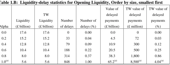
Here we first implement the Bech-Soramäki (2002) methodology for determining the liquidity-delay trade off in RTGS where all liquidity is posted up front at opening and liquidity-delayed payments are settled on a FIFO basis. To do this, we run a simulation of our OL system where the banks are assumed to post liquidity based on equation (11) above for each of the six values of . Table A gives the results of these simulations. Table B, in contrast, reports the results for the OL system when banks submit the payments for settlement smallest in value first. Again we run six simulations based on different values of . What is interesting is that as the OL system is squeezed for liquidity, i.e., when liquidity posted is at the lower bound value, there are some 10 unsettled payments of about £7.8 billion when banks reorder payments for settlement based on their value. In particular, two banks needed to make six and four payments to each other,
respectively. As neither had an adequate settlement balance to make the smallest payment they owed the other, we were left with a gridlock situation in which £7.8 billion of payments were left unsettled. In the FIFO case for the OL system, there was no gridlock. Further, at liquidity levels equal to the lower bound the time-weighted value of delayed payments in Table1.B is over twice that of the case in Table 1.A when banks follow the FIFO rule.
Table 1.A: Liquidity-delay statistics for Opening Liquidity, FIFO
Alpha Liquidity (£ billion) TW Liquidity (£ billion) Number of delays Number of delays (%) Value of delayed payments (£ billion) TW value of delayed payments (£ million) TW value of delayed payments (%) 0.0 17.6 17.6 0 0.00 0.0 0 0.00 0.2 15.2 15.2 60 0.07 4.7 68 0.03 0.4 12.8 12.8 303 0.36 12.3 229 0.11 0.6 10.4 10.4 796 0.94 23.2 503 0.24 0.8 8.0 8.0 3370 3.98 49.2 1,279 0.61 1.0 5.6 5.6 12319 14.54 87.6 3,804 1.80
Table 1.B: Liquidity-delay statistics for Opening Liquidity, Order by size, smallest first
Alpha Liquidity (£ billion) TW Liquidity (£ billion) Number of delays Number of delays (%) Value of delayed payments (£ billion) TW value of delayed payments (£ million) TW value of delayed payments (%) 0.0 17.6 17.6 0 0.00 0.0 0 0.00 0.2 15.2 15.2 33 0.04 4.5 72 0.03 0.4 12.8 12.8 79 0.09 10.9 300 0.12 0.6 10.4 10.4 188 0.22 20.5 500 0.25 0.8 8.0 8.0 314 0.37 38.3 1,800 0.86
1.0(a) 5.6 5.6 848 1.00 65.2(a) 8,500(a) 4.04(a)
(a) Includes value of the 10 failed payments totalling £7.8 bn.
These results are in line with some unpublished work that two of the authors carried out using the BoF PSS. They suggest that if the system operators are worried about controlling operational risk by minimising the total value of payments in the queue, they would always prefer banks to use the standard FIFO by priority method of sorting their payments. If, alternatively, they were most concerned about the volume of payments in the queue, they would always prefer the banks to use the ‘order by size, smallest first’ method of sorting their payments. In practice, banks choose to post far more liquidity than the lower bound value (indeed they post far more liquidity than the upper bound value), probably to counter the possibility of being unable to make time-sensitive payments. In particular, this is more likely to be the economical option when liquidity costs are relatively low and posting additional liquidity would not make large inroads into bank profitability. In addition, it is also likely that in a gridlock situation the banks concerned would negotiate an interbank loan so as to enable one bank to make the first payment needed for the gridlock situation to unwind; this possibility was not considered in our experiment.
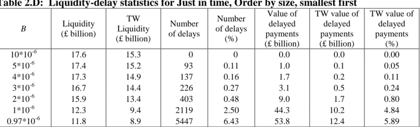
Tables 2.C and 2.D report the liquidity-delay trade offs for the JIT system conditional on different threshold values for b. With b = 6*10-6, banks will make all payments without delay. To do this, they need to use a total of £17.6 billion, the ‘upper bound’ value of liquidity needed by the system. With b = 0.97*10-6 (at which point liquidity used is minimised), banks use a total of £11.9 billion if they order their queues by FIFO and £11.6 billion if they order their queues by value. At all levels of liquidity, fewer payments are delayed when queues are ordered by value than when they are ordered by FIFO but the value of delayed payments is higher when queues are ordered by value than when they are ordered by FIFO. This is the same as we found for OL systems and again suggests that if the system operators are worried about controlling operational risk by minimising the total value of payments in the queue, they would always prefer banks to use the standard FIFO by priority method of sorting their payments.
Table 2.C: Liquidity-delay statistics for Just in time, FIFO
B Liquidity (£ billion) TW Liquidity (£ billion) Number of delays Number of delays (%) Value of delayed payments (£ billion) TW value of delayed payments (£ billion) TW value of delayed payments (%) 10*10-6 17.6 15.3 0 0.00 0.00 0.00 0.00 5*10-6 17.5 15.2 102 0.12 0.97 0.10 0.05 4*10-6 17.3 15.0 155 0.18 1.33 0.20 0.09 3*10-6 16.8 14.4 258 0.30 2.81 0.44 0.21 2*10-6 15.8 13.4 470 0.55 8.56 1.50 0.71 1*10-6 12.5 9.5 2845 3.36 43.90 10.01 4.74 0.97*10-6 11.9 9.1 6089 7.19 52.29 11.93 5.65
Table 2.D: Liquidity-delay statistics for Just in time, Order by size, smallest first
B Liquidity (£ billion) TW Liquidity (£ billion) Number of delays Number of delays (%) Value of delayed payments (£ billion) TW value of delayed payments (£ billion) TW value of delayed payments (%) 10*10-6 17.6 15.3 0 0 0.0 0.0 0.00 5*10-6 17.4 15.2 93 0.11 1.0 0.1 0.05 4*10-6 17.3 14.9 137 0.16 1.7 0.2 0.11 3*10-6 16.7 14.4 226 0.27 3.1 0.5 0.24 2*10-6 15.9 13.4 403 0.48 9.0 1.7 0.80 1*10-6 12.3 9.4 2119 2.50 44.3 10.2 4.84 0.97*10-6 11.8 8.9 5447 6.43 53.8 12.4 5.89
Figure 1 below graphs the percentage time weighted value of delayed payments against the liquidity posted in the OL and JIT systems.
Figure 1: Trade off between Liquidity posted and Time Weighted Delays
5.2 The impact of operational events in the two systems
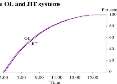
As we said earlier, one way of gauging the effect of an operational event is to examine how quickly payments are submitted to the central processor and settled within the system. The logic is that should an operational event occur, it will affect the ability of the system to sort out any remaining payments for the day. The more payments that have already been processed before the event happens, the less this will be a problem. Figure 2 shows the throughput for the two
systems, viz. the percentage of payments by value that are settled prior to any given time for each of our two systems. To make the comparison fair, we assumed that £12.8 billion of liquidity was used in each of the two systems. From Tables A and C, respectively, we see that in the FIFO case, at this level of liquidity, the JIT system delays £44.8 billion worth of payments with time weighted value of £10.2 billion. In contrast, the OL system delays payments valued at about £12.3 billion with time weighted value of £0.2 billion. Chart 1 shows that, at each point in time, the OL system has settled more payments than the JIT one.
Time weighted delay vs. Liquidity
£0 £5 £10 £15 £20 £25 0.00% 1.00% 2.00% 3.00% 4.00% 5.00% 6.00% 7.00% 8.00% 9.00% 10.00%
Percentage TW delay value
L iqu idit y po sted ( b illi o n s)
OL SIZE OL FIFO JIT SIZE JIT FIFO OL (Delay by size)
OL (FIFO)
JIT (Delay by size)
0 20 40 60 80 100 5:00 7:00 9:00 11:00 13:00 15:00 T ime Per cent
Chart 1: Throughput in
the OL and JIT systems
OL JIT
Figure 2: Through put (%) of payment requests settled with X-axis giving time of day
6. Erev- Roth reinforcement learning by banks to post optimal liquidity (alpha): Opening Liquidity system
Here we report the results on how banks can endogenously learn to determine how much liquidity to post. For this we use the Erev- Roth reinforcement learning (RL) algorithm (Erev and Roth (1998)) which is known to be a powerful learning device and has been successful in training artificial agents on how to play complex games. RL is an experientially driven low rationality algorithm that enables agents to develop sufficient competence to play strategies that will, with a high probability, enable them to play optimally with little or no knowledge of the characteristics of other agents and of the environment itself.
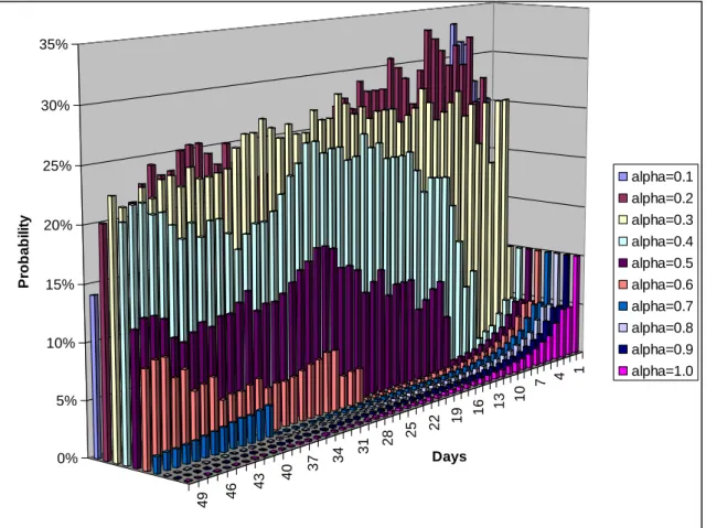
The choice of strategy here involves different values of alpha in equation (11) which enables a bank to minimize liquidity and delay costs given that other banks are behaving similarly. We assume the first in first out (FIFO) ordering of payment requests. Figure 3 gives the result of 50 days of learning for a single bank where initially the possible values of alpha (from 0 to 1) are placed in 10 alpha ‘buckets’. The picture below shows how the probabilities of a particular bank using each of the possible alpha values evolve over time as the bank learns. It starts at Day 1 with all buckets having the same probability of 10%. In this particular instance, the bank seems to learn that using lower values of alpha is more profitable, so the probabilities of using large values of alpha quickly decrease to negligible values. As can be seen from Figure 3, after 50 days, the alphas that the bank is more likely to use are between 0.3 to 0.4. Note: this is only one particular example, and the results are highly dependent on the relative magnitudes of liquidity costs vs. delay costs.
Figure 3 shows how a single bank learns to determine the alpha parameter. If we average the alpha used by all banks in each day, we see that over the 50 day period, the average alpha value for this particular simulation tends to decrease to about 0.35. This is shown in Figure 4. This implies that banks learn to operate at about £12-£13 bn levels of opening liquidity which shows very high efficiency in terms of a less than 0.1% time weighted delay in payments (see Table 1.A).
1 4 7 10 13 16 19 22 25 28 31 34 37 40 43 46 49 0% 5% 10% 15% 20% 25% 30% 35% P ro b a b il it y Days alpha=0.1 alpha=0.2 alpha=0.3 alpha=0.4 alpha=0.5 alpha=0.6 alpha=0.7 alpha=0.8 alpha=0.9 alpha=1.0
Figure 3: Results of Erev-Roth Reinforcement Learning over 50 days of how much liquidity to post (alpha) at the beginning of the day : A single bank case
0 0.1 0.2 0.3 0.4 0.5 0.6 1 3 5 7 9 11 13 15 17 19 21 23 25 27 29 31 33 35 37 39 41 43 45 47 49 Day A v e ra ge a lph a a c ros s ba nk s
Figure 4: Results of Erev-Roth Reinforcement Learning over 50 days of how much liquidity to post (alpha) at the beginning of the day :Averaged over all banks
7 Concluding remarks and future work
In this paper, we have discussed a methodology for simulating interbank payment systems that is capable of handling real time payment records along with limited autonomy in bank behaviour. We showed that this methodology could be used, in principle, to evaluate different designs of RTGS systems by carrying out an example experiment using two systems: one in which liquidity was posted at the beginning of the day and one where it could be borrowed ‘just in time’.
In RTGS systems, payment requests to banks are not fully and individually financed as then they would need an amount of liquidity equal to the total value of payments made; rather, the bulk of the liquidity used for settling comes in the form of incoming payments. The efficiency in recycling the liquidity posted by banks is the key to the design of RTGS system. At the level of individual banks, an attempt to handle the trade-off between liquidity and delay costs may result in behaviour where banks delay settlement in anticipation that other banks will make payments to them first. Thus, in principle banks always have the discretion to reorder payments for
submission at the central processor influencing the liquidity that they need to post and the ability of the system to settle payments. What appears to be an individually rational response at the level of banks, viz. to delay large payments (with low priority), leads to a deterioration in the collective performance of the RTGS system whether in the OL case or the JIT variant. However, we found that the JIT system is more prone to rapid deterioration of its liquidity recycling capabilities than the OL system. In fact, a key message of our experiments is that, at any given level of liquidity, the JIT system would generate more delayed payments than an otherwise identical system in which banks posted their liquidity at the beginning of the day, and this would be bad from an operational risk point of view.
However, some important caveats need to be borne in mind in the interpretation of the results of our experiment. In particular, our experiments relied on one particular stochastic simulation of data based on one day’s worth of actual payments. To get a clearer picture we would need to run multiple simulations based on data from a large number of days. In addition, our experiments on the OL system imposed a given level of opening liquidity. In order to get a real understanding of how such systems work, one would need to postulate behavioural rules to explain the decision of how much liquidity to post at opening and allow the parameters of such rules to depend on the outcomes of previous days. For the JIT system, we assumed that banks did not take into account the possibility of using liquidity from incoming payments to make their own future payments when they choose how long to delay payments.
The main issue relating to mechanism design in real time interbank settlement systems is the question ‘At what levels of liquidity and delay will each system operate? In particular, we would like to know how the socially efficient outcome can be achieved by design, with banks having to behave autonomously and faced by asymmetric information. In the philosophy of agent based modelling, however, the prior question is ‘Can banks behaving autonomously adaptively learn to achieve the liquidity savings associated with cooperative outcomes?’ An obvious extension of the work presented in this paper would be to focus on the question of whether or not banks, as autonomous and adaptively intelligent agents playing a repeated game, can move to the efficient
and stable point of the ‘good’ equilibrium; that is, could they co-operate in such a way as to enable them to make payments with little delay in an OL system operating at liquidity levels close to the lower bound. Preliminary results in Section 6 based on adaptive learning by banks show that they could in fact operate without much free riding at very high efficiency with few delayed payments. Computational experiments of this kind can yield invaluable normative insights into the complex intraday liquidity management game by banks within the context of bank profitability and solvency. For this further experimentation is needed using Erev-Roth type autonomous learning over multiple days and under different market conditions to see if banks’ liquidity strategy changes. Finally, it will be interesting to see how banks respond to changes in policy rules of RTGS. Wind tunnel tests for proposed policy changes such as the introduction of hybrid large value payment systems which combines RTGS and real time netting requires an artificial test bed of this kind.
References
Angelini, P (1998), ‘An analysis of competitive externalities in gross settlement systems’,
Journal of Banking and Finance, Vol. 22, pages 1-18.
Bank of England (2000), Oversight of payment systems.
Bank for International Settlements (2003), A glossary of terms used in payments and settlement systems.
Bech, M L, and Soramäki, K (2002), ‘Liquidity, gridlocks and bank failures in large value
payment systems’, in R. Pringle and M. Robinson (eds.) E-Money and Payment System Review, London: Central Banking Publications.
Bech, M L, and Garratt, R (2003), ‘The intraday liquidity management game’ Journal of Economic Theory, Vol. 109, pages 198-219.
Bedford, P, Millard, S P, and Yang, J (2005), ‘Analysing the impact of operational incidents in
large-value payment systems: A simulation approach’ in Leinonen, H. (ed.), Liquidity, risks and speed in payment and settlement systems: A simulation approach, Bank of Finland.
Erev, I., Roth, A., (1998), Predicting how people play games: reinforcement learning in
experimental games with unique, mixed strategy equilibria, American Economic Review, 88, 848-881
Leinonen, H, ed. (2005), Liquidity, risks and speed in payment and settlement systems: A simulation approach, Bank of Finland.
Lester, B, Millard, S P, and Willison, M (2005), ‘Optimal settlement rules for payment systems’, Bank of England, mimeo.
McAndrews, J (2005), ‘Current trends in payment systems: A microstructure approach’, paper
given at a Bank of England conference on ‘The future of payments’, May 19 and 20, 2005.
McAndrews, J, and Rajan, S (2000), ‘The timing and funding of Fedwire funds transfers’,
Federal Reserve Bank of New York Economic Policy Review, July, pages 17-32.
McAndrews, J, and Trundle, J (2001), ‘New payment system design: Causes and consequences’, Bank of England Financial Stability Review, December, pages 127-36.
Willison, M (2005), ‘Real-time gross settlement and hybrid payment systems: A comparison’,