Department of Economics Issn 1441-5429 Discussion paper 03/11
A q Model of House Prices
1Jakob B. Madsen2
Abstract:
This paper develops a Tobin’s q model of house prices which shows that changes in interest rates, demography, and income are likely to have only temporary effects on house prices while house prices in the long run are determined by prices of developed land, value added taxes, stamp duties, and construction costs. Empirical estimates show that agricultural land prices are a proxy for urban land prices, which, together with construction costs are the key determinants of house prices in the long run.
Key words. housing market, Tobin’s q, construction costs, land prices JEL. E130, E220, G120
1
Helpful comments and suggestions from Greg Scwann, Dan Knudsen, Jonathan Pincus, Torbjorn Lange and participants at seminars at the University of Western Australia, Curtin University, Deakin University, University of Victoria, Wellington, The Reserve Bank of New Zealand, and Monash University, are gratefully acknowledged. Hui Yao provided excellent research assistance.
2
Department of Economics, Monash University Australia. Jakob.Madsen@monash.edu +613 9903 2134
© 2011 Jakob B. Madsen
All rights reserved. No part of this paper may be reproduced in any form, or stored in a retrieval system, without the prior written permission of the author.
1 Introduction
Important progress has been made in modeling house prices over the past decades. In the first generation models of Muth (1960), Huang (1966), and Smith (1969) demand for housing depends on the real price of housing, the alternative cost of renting, and user costs, among other variables. Expected capital gains and tax deductibility of interest payments are absent from these models. In the second generation models of Kearl (1979), Buckley and Ermisch (1982), Dougherty and Van Order (1982), and Poterba (1984) expected capital gains and tax considerations were incorporated into user costs and became a central part of house price models. The second generation models of house prices have been widely used in the empirical literature (see for example Mankiw and Weil, 1989, Meen, 1990, 2002, Tsatsaronis and Zhu, 2004, and Girouard et al. 2006).
The problems associated with the existing models of house prices are that they are of partial equilibrium nature and, therefore, do not adequately capture the interactions between the asset markets, demand for housing services, and the market for residential investment. Although Poterba’s (1984) model allows for the interaction between the capital accumulation constraint and the present value of rent/house services, the model does not allow for optimizing firm behavior and, consequently, residential property investors do not respond in an optimizing manner to disequilibrium in the housing market.
A related problem associated with the existing models is that they have not adequately established the factors that determine the long run equilibrium of house prices. Variables to which house prices gravitate towards in the long run have been used in the literature. Examples of these variables are nominal housing rents, discounted nominal housing rents, (per capita) nominal income, particularly, wealth and population multiplied by consumer prices and other deflators.3 Applying Tobin’s q theory to the housing market Summers (1981), Poterba (1991), Abraham and Hendershott (1996), and Shiller (2006) assume that the shadow costs of houses equal construction costs and, therefore, that building investment will close the gap between the market value of houses and construction costs.4 However, since the cost of structures in most metropolitan areas, in which the supply of land is quite inelastic, is only a fraction of the total cost of new houses (Capozza and
3 See for, example, Meen (1990, 2002), IMF (2004), Tsatsaronis and Zhu, (2004), Gallin (2004, 2006), OECD (2005), and particularly Table 3 in Girouard et al. (2006). Gallin (2006) argues that while income is widely used as the long-run determinant of house prices, income and house prices are not cointegrated, not even in panels with 95 metropolitan areas over 23 years.
4 Meen (2002) notes that construction costs are rarely used in British studies while it is more commonly done in US studies.
Helsley, 1989) the value of residential land needs to be allowed for in order to generate a theoretically and empirically satisfactory account of the shadow value of the housing stock.5
The contribution of this paper is partly theoretical and partly empirical. In the theoretical part of the paper a model of optimizing firm behavior is used to show the factors that determine house prices on short run and long run frequencies under the assumptions of exogenous interest rates (Section 2). The model extends the model of Poterba (1984) by allowing for optimizing behavior among investors and by allowing for the influence of value added taxes and stamp duties in the optimization. The theory shows that house prices in the long run, are determined by construction costs, land values, value added taxes, and stamp duties. While taxes traditionally influence house prices through the channel of user costs, it is shown that taxes influence house prices in the long run through the channel of acquisition costs of houses and, therefore, have effects on house prices that are quite different from that of user-cost-based models. In Section 3 the model is extended to allow for consumers that optimize intertemporally in a general equilibrium setting. The theoretical hypothesis developed in Section 2 is supported by the estimates, which show that house prices, in the long run, are driven by land prices, construction costs, value added taxes and stamp duties taxes using long historical data for 6 industrialized countries (Section 4). The macroeconomic implications of the findings for international transmissions of business cycles and the assessment of the fundamental value of house prices are discussed in Section 5.
2 The model
This section derives a supply side model of house and property prices under the assumption that the interest rate is determined exogenously by other countries under a fixed exchange rate regime or by the monetary authorities under the regime of floating exchange rates. It is shown that house prices in the short run are determined by portfolio equilibrium while they are determined by replacement costs in the long run. The assumption of exogenous interest rates is relaxed in the next section. Throughout the paper house prices will refer to the price of structures plus the price of land.
Consider the profit maximization problem of the individual investor, where all the variables are in units of individuals:
5 Although land prices are sometimes mentioned in the literature as potentially important components of acquisition costs of housing, as for example by Evans (2004), they are hardly ever included in econometric modeling, where Poterba (1991) is one of the few exceptions. Poterba (1984) incorporate land prices into his model, however, he does not explicitly incorporate land prices as a determinant of the shadow price of houses.
( )
(
)
(
)
{
}
∫
∞ = − Φ − + + + = ∏ 0 1 1 ] ) / ( [ max t i t t t t t t t rt dt h h h I h H e ψ & μ τ , (1) st t t t I h h& = −δ , (2)where r is the required returns to housing investment, H is the economy-wide housing stock, Φ(H) is the marginal revenue per unit of housing stock which is a declining function of the economy-wide stock of the housing, h is the housing stock of the individual builder or the individual household, I is real gross residential investment per individual, ψ(h&t/ht)htis adjustment cost of housing investment,
where ψ(0)=0, ψ'(h&t/h) > 0, ψ''(h&t /h)> 0, δ is the depreciation rate, τi
is the value added tax rate, and μ is stamp duties as a percentage of acquisition costs. A dot over a variable signifies the time-derivative. Value-added taxes are, as a rule, paid on construction costs and land for new houses and for maintenance and renovations. Sales of second-hand houses are not subject to sales taxes. Investment and investment adjustment costs are kept in real values although taxes apply to nominal values to keep the exposition as simple as possible and without affecting the principal results.
The required returns are given by r=i(1−θ), where i is the nominal interest rate, and θ is the income tax rate. Property taxes are omitted from the required returns and interests are assumed to be fully tax deductible for simplicity although interests are not tax deductible in all countries and some countries use a fixed rate for tax deductions that is below the income tax rate. Below r is referred to as required returns while uc = r + is referred to as user costs, where is the depreciation rate. User costs are derived formally from the consumer’s intertemporal optimization problem in Section 3. Depreciation is not included as a determinant of r, because depreciation is allowed for in the capital accumulation constraint.
Maximizing (1) under the capital accumulation constraint given by (2) yields the following first order conditions:
(
)
[
]
(
)
( )
i t t t t h t t t t r q H I h q& =( +δ
) −Φ( )+ψ
−ψ
' / 1+μ
1+τ
, (3)(
)
(
)
⎥⎦⎤ ⎢ ⎣ ⎡ − + + = − 1 1 1 '1 i t t t t t q h h τ μ ψ & , (4)0 lim − = ∞ → t t rt t e qh , (5)
where q is the shadow price of housing stock or Tobin’s q, which is discussed in depth in subsection 2.1 below. Equations (3) and (4) define a simultaneous first–order differential equation system and Equation (5) is the transversality condition, which ensures that the present value of the total housing stock at infinity is zero. Equation (4) is net investment in residential buildings. In a no-tax world this equation collapses to the traditional Tobin’s q model in which investment is positive if q >1 and vice versa. A value of q higher than 1 is required for investment to be positive because taxes increase the effective acquisition costs of investment as discussed in the next subsection.
The asset market equilibrium condition given by (3) is most easily interpreted if it is rewritten as
(
)
[
]
(
)
(
)
t i t t t t h t t q h I H q q r ⎟⎟ ⎠ ⎞ ⎜⎜ ⎝ ⎛Φ − − + + + ⎟⎟ ⎠ ⎞ ⎜⎜ ⎝ ⎛ = +δ & ( ) ψ ψ' / 1 μ 1 τ ,i.e. user cost of capital is equal to relative capital gains/losses plus dividend yield in portfolio equilibrium. In other words, the returns to investing in residential housing are equal to the rent or housing services as a percentage of the shadow cost of capital plus the expected capital gain/loss on the investment as a percentage of capital outlay minus depreciation expenses.
2.1 Shadow price of residential property
The shadow price of housing stock, q, is given by the ratio of the current market value of an additional unit of housing stock to its replacement costs. Provided that the usual homogeneity assumptions are satisfied, the marginal q equals the average q (Hayashi, 1982). Conventionally Tobin’s q for housing is measured as house prices deflated by construction costs (Summers, 1981, Poterba, 1991, Abraham and Hendershott, 1996, and Meen, 2002). However, the cost of the structure is often only a fraction of the land price of the property (Capozza and Helsley, 1989). Thus the replacement cost of houses is an average of construction costs and the cost of developed land.
These considerations suggest that the shadow price of the housing stock is given by:
) 1 ( α α − = t t h t t cc lc p q , 0 0, (6)
where ph is the price of a unit of housing, lc are the costs of developed land per unit of housing and cc are construction costs per unit of housing.
Unfortunately, the price of developed land is rarely available and when available, tends to be of poor quality, and what’s more, does not solve the fundamental question of what factors determine house prices. Therefore, a theory of factors that determine the price of developed land is called for. Urban growth theory suggests that residential land values are determined by agricultural land values, the costs of developing the land for urban use, the expected increase in rents and the value of the accessibility to the central business district (Capozza and Helsley, 1989). Wheaton (1974) shows, more formally, that land is developed for housing until the urban land gradient intersects agriculture rent at the edge of the city in equilibrium. As urban areas grow the land rents are pushed up throughout the city, which in turn, leads to an expansion of land for development at the edge of the city. It follows that house prices are determined by construction costs, agricultural land prices, and development costs that are not related to construction costs. The question is whether a combination of construction costs and agricultural land prices, at least for some countries, can be used as a proxy for repurchase prices of houses.
The prices of agricultural land is only a fraction of the price of developed land (Shiller, 2006) and the absence of suitable or available land around some larger cities will effectively constrain the supply of developed land. For the former territory of the Federal Republic the price per square meter of undeveloped and developed land was 31.12 and 140.44 EURO, respectively, in 2005. Assuming that the average size of a “house-sized” plot of developed land is 500 m2 the cost of developed land is 70,220 EURO.6 This is a significant fraction of the average total cost of a house, which was 113,661 EUROs in 2004 (Girouard et al., 2006).
A question is whether the price of developed land varies proportionally to the price of agricultural land prices and, therefore, whether agricultural land prices can be used as proxies for costs of developed land in locations where the supply of land is not constrained. Theoretically, the prices of developed land at the fringe of the city are heavily influenced by prices of agricultural land. Suppose house prices in the outer circles of a city increase due to increasing prices of agricultural land. This makes houses closer to the city center relatively more affordable and leads to an excess
demand for these houses. Thus, due to ripple effects, house prices in the whole city are pushed up by the initial increase in prices of agricultural land.
Empirically, Statistik Bundesamt and Told & Skat publish data on average purchasing value per square meter of developed building land and undeveloped building land in Denmark and Germany.7 Regressing the log of the price of developed building land on the log of the price of undeveloped building land over the period from 1962 to 2005 for Germany and over the period from 1938 to 2007 for Denmark yield the coefficients of the log of undeveloped land of 1.09(7.31) and 0.67(11.91), where the number in parenthesis is the t-statistics. The dynamic OLS, as discussed below, is used in the estimates. These results suggest that the price of developed land in Germany and Denmark approximately vary proportionally to the price of undeveloped land. However, these results may not apply to other countries and, therefore, whether agricultural land prices are suitable proxies for the cost of developed land remains an empirical issue, which is addressed in the empirical section.
In the short run the supply of land is likely to be restricted by tough zoning rules, burdensome building restrictions, and lengthy administrative procedures (see Girouard et al., 2006, for examples for the US, the UK and Ireland). In the long run, however, the supply will, in most events, adjust to demand as builders work their way through the administrative apparatus and new zoning rules are introduced. Furthermore, delays may give developers an incentive to increase their stock of developed land to meet unexpected demand and, therefore lead to a faster supply response than in an unregulated market.
2.2 House prices in the long run
Solving Equations (4) and (6) in steady state gives the determinants of house prices in the long run: ) 1 ( * ) 1 )( 1 ( +μ +τ α −α = lc cc pth t ti , (7)
where an asterisk refers to steady state. This equation is the key equation in this paper and shows that house prices in steady state follow the direct acquisition costs (land and construction costs), stamp duties and value added taxes because they represent the effective replacement costs of houses. Stamp duties and value added taxes increase the effective acquisition costs of houses and, therefore, permanently increase house prices.
Stamp duties vary substantially across countries and over time. Stamp duties are almost 6% of the sales prices of property in the state of Victoria, Australia, and 4% of the sales prices of property in Finland, and are somewhat lower in most other OECD countries. Historically, stamp duties have been a significant fraction of house acquisition costs and may have played a potentially important role in the movements of house prices in the past. Stamp duties were the main source of tax revenue in the 17th and the 18th century in Europe and the US and were a significant part of the tax revenue in the 19th century in Europe and the US (van der Poel, 1954).
In contrast to the conventional analysis of housing prices, the price of housing in the long run is independent of the interest rate. This is because investors set the returns they require on their investment and the housing stock adjusts endogenously until the expected returns equal the required returns, as shown more explicitly in the next section. However, there are three channels through which the interest rate or the required returns may permanently affect house prices. First, if the land supply is not perfectly elastic e.g. in places such as Hong Kong, Japan, Singapore, and other big cities, the capitalisation effects of permanent real interest rate changes have permanent effects on house prices. Second, land prices are determined by the present value of yield per acre provided that the supply of marginal land is inelastic. Some land price models assume that yields are discounted by a fixed real discount rate while others allow the discount rate to vary over time (see for example Hardie et al., 2001, and Roche and McQuinn, 2001). Thus the price of agricultural land may or may not be influenced by the real interest rate. Third, nominal interest rates affect financing costs throughout the period in which housing is build and, therefore, increase the effective acquisition costs of houses. Since empirical evidence suggests that the real interest rate is mean-reverting (Koustas and Lamarche, 2006), the interest rate is unlikely to be important for house prices in the long run.
The model is quite different from the models of Poterba (1984) and Mankiw and Weil (1989) in which capital adjustment is not derived from optimising behaviour among investors but is assumed to be related to the following equation: H& =ψ(qt)−δH. In contrast to the model in this paper, demand shocks and demographic shifts have long-term effects in their models, even if the supply of land is perfectly elastic, because the supply schedule is upward sloping as the capital depreciation expenses increase along with higher housing stock. The model in this paper is also quite different from the model of Dougherty and Van Order (1982), which is widely used in the literature.8 Since
8 Note that Dougherty and Van Order (1982) present two separate models; one which is derived from intertemporal consumer optimizing behavior and one that is derived from the firm’s profit maximizing problem.
investment adjustment costs are not allowed for in their model the investment function and, therefore, the capital adjustment is not identified. Consequently, their model is more a short-term than a long-term model of housing prices.
2.3 Dynamic effects of various shocks on house prices
This section shows the effects on house prices and housing stock of changes in interest rates, inflation, taxes, demand, demography, and land prices and the results are compared to the results obtained in the literature.
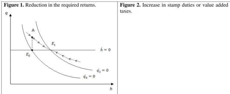
Figures 1-3 show the dynamics of the simultaneous first-order differential equation system given by (3) and (4). The q&=0 and h&=0 schedules are given by the following equations:
δ + Φ = t t t r H q ( ) , (8) ) 1 )( 1 ( t ti t q = +μ +τ , (9)
where the q&=0 schedule is downward sloping because housing services and rents are declining functions of the housing stock. Note that (8) defines q as the present value of housing services or rent under the assumption that rent and the interest rate at period t are expected to remain constant to infinity.
Figure 1. Reduction in the required returns. Figure 2. Increase in stamp duties or value added taxes.
Figure 1 shows the effects of an unexpected real interest-induced reduction in the real required returns. Starting from the steady state equilibrium at the point E0 the q&0 =0 schedule shifts to the right (more correctly it changes slope) and the perfect foresight house market jumps to the point A because housing rents/services are capitalized at a lower discount rate. The perfect foresight market will not jump the whole way up to the q&1=0 line, because it knows that the increased present value of housing rent will only last for the period in which the housing stock remains fixed. Since q exceeds it’s equilibrium value at the point A it is profitable to build new houses and the housing stock starts increasing. The increasing housing stock will increase the supply housing, which in turn will reduce the rental income per unit of housing; thus bringing down q towards its long run value. Under the assumption that the developers financing costs are not influenced by the interest rate reduction, the shadow price of houses remains unaffected by interest rates in the long run. Whether house prices in the long run are affected by the reduction in the required returns depends entirely on land supply elasticities. If the supply of developed land is perfectly elastic and determined by the supply of agricultural land, house prices will be unaffected by the interest changes in the long run. Conversely, if the supply of land is inelastic house prices will be affected by interest rate shocks and demand shocks even if the h&=0 schedule is horizontal. This issue is addressed in the empirical section.
The role of demand shocks and demographic shifts is indirect in the model. Assuming that housing rent is a positive function of demand factors such as income and the proportion of the population in the 25-35 years age group, a positive unexpected shift in demand or the demographic
composition leads to a rightward shift in the q&=0 schedule. Another channel through which demand can influence house prices is via demand for office space that may spill over to the housing market as these two sectors are competing for space. The dynamics are similar to the dynamics in Figure 1. From the dynamics it can be concluded that the shifts in demand and in demography have only short term effects on Tobin’s q because the adjustment of the housing stock will continue until the shadow price of houses are brought down to their initial level.
The gap between housing prices and repurchases costs created by positive demand shocks may be reduced by increasing construction costs because of Philips curve effects and by higher agricultural land prices that may be positively affected by land development (see, for estimates, Hardie et al., 2001). In the long run, however, demand shocks have no effects on land prices and construction costs provided that a buffer of agricultural land is available in the economy. Agricultural land prices are unlikely to be affected by land development in the long run because agricultural land prices are determined by yield per acre, which is in turn determined exogenously by world agricultural prices and technological progress.9 Furthermore, neither demand nor supply shocks will influence construction costs in the long run following the natural rate hypothesis in which wage-induced unemployment will put downward pressure on the wage growth rate until the pre-shock equilibrium wage is re-established.
Since real agricultural land values have fluctuated substantially over the past four decades they have been a potentially important source of house price fluctuations given that prices of developed land, at least for Germany and Denmark, tend to follow the price of undeveloped land. The increasing real value of land in the 1970s can be attributed to the food price hike during the same period (see for instance Lindert, 1988). Suppose that increasing prices of agricultural produce unexpectedly increase land prices. This leads to increasing acquisition costs of houses and a corresponding instant increase in the price of houses to maintain q at its steady state level. Thus neither the q&=0 schedule nor the
0
=
h& schedule is affected by the change in land prices. The same conclusion holds for changes in real construction costs.
Next, consider an unexpected increase in stamp duties or value added taxes, which shift the 0
=
h& schedule up from h&0 =0 to h&1=0 in Figure 2. In other words, stamp duties and value added
9 Mundlak et al. (1997) find that real prices of agricultural land have hardly increased over the past century for four countries for which they were able to find long data. This result suggests that the increasing income during the last century had no long-term effects on agricultural land prices.
taxes have increased the effective acquisition costs of houses, thus pushing house prices up. House prices jump to the point A and follow the stable saddle path towards the new long run equilibrium at E1 as the stock of housing is being reduced. Although house prices will increase, the existing house owners will only experience a capital gain in the case of increasing value added taxes. Existing house owners will not experience a capital gain in the event of increasing stamp duties since the increasing taxes have created a wedge between the price paid by the new house owner and the price received by the vendor.
Finally, the question is whether supply elasticities are sufficiently large to prevent demand shocks from having permanent effects on house prices. Girouard et al. (2006) find that there is a small significant positive relationship between building activity and the ratio of house prices to the housing investment deflator in the OECD countries, which suggests that the supply side adjusts to disequilibrium in the housing market. That the relationship is not strong may reflect that land prices have not been allowed for in their estimates of Tobin’s q.
3 Endogenous discount rate
In the last section it was assumed that house prices were solely determined by the investment decision and that the provision of house services, consequently, played no role in the determination of house prices. This section relaxes the assumption of an exogenous discount rate in the previous section by allowing households to optimize intertemporally. The extension is important because the dual role of housing investment as being a simultaneous demand for assets and demand for housing services for the potential owner occupier. In general equilibrium there must be simultaneous equilibrium in asset and housing markets. This duality is explicitly acknowledged in this section.
Consider the representative consumer who maximizes the following constant-relative-risk-aversion CRRA utility function:
∫
∞ = − − − ⎥ ⎦ ⎤ ⎢ ⎣ ⎡ − + = 0 1 1 0 1 ) ( max t t t t dt h c e U γ ϕ γ γ ρ , (10)(
)
(
)
t t t t t t t t i t t t t t x t t P I h h h c y i b b b& + [ +ψ(& / ) ]1+μ 1+τ + =(1−θ ) +(1−θ ) ⋅ −π , (11)where b is financial savings per individual, ρ is the subjective time-preference, π is expected inflation, y is real income of the individual, Px is the price of a house relative to prices of non-durable consumer goods, c is consumption of non-durables per individual, and γ is the coefficient of the relative risk aversion or the inverse intertemporal rate of substitution. The term πtbt is the real
depreciation of bonds, i.e. inflation erodes the real value of bonds. The value of bonds is the net financial asset position (including mortgage debt) of the individual. The flow of housing services is assumed to be proportional to the stock of housing, where ϕ is the constant of proportionality. The right hand side of (11) is the sum of after-tax income and real interest income. Interest income will be negative if the mortgage debt exceeds the individual’s net holding of other financial assets. The left-hand side of (11) is the sum of consumption, gross investment in housing, and net savings.
Defining qtA as the shadow value of housing stock the Hamiltonian is given by the equation:
(
1)
(
1)
(1 ) [ (1 ) ] ] ] ) / ( [ [ 1 ) ( ) , , ( 1 1 t t t t t t t i t t t t t x t t A t t t t A b i y c h h h I P b q h c e q h c ⎥+ + + + + + − − + − − ⋅ ⎦ ⎤ ⎢ ⎣ ⎡ − + = ℜ − − − ψ μ τ θ π θ γ ϕ γ γ ρ & &Maximizing the Hamiltonian yields the following first order conditions:
0 = ∂ ∂ℜ c : + =0 − − A t t t q c e ρ γ (12) A t q h =−& ∂ ∂ℜ :
(
)
[
]
(
)
(
)
A t i t t t t h x t A t t t q h I P q h e−ρϕ(ϕ )−γ + ψ −ψ' / 1+μ 1+τ =−& , (13) A q b =−& ∂ ∂ℜ : A t t t t A t i q q [(1−θ ) −π ]= & , (14)Taking logs of Eq. (12) and differentiating with respect to time yields:
ϑ γ ρ+ ≡ = • t t A A c c q q& / (15)
where ϑ is the returns to consumption. Substituting Eq. (15) into Eq. (13) yields the Euler equation: ) 1 /( θ ϑ − = i (16)
Combining Eqs. (12), (13) and (14) yields the following expression:
(
)
[
/]
(
1)
(
1)
(1 ) ] [ 1 ' t t t i t t t t h x t t t i h h P c h ψ ψ μ τ π θ ϕ ϕ γ = − + + − + − ⎟⎟ ⎠ ⎞ ⎜⎜ ⎝ ⎛ − & . (17)This equation says that the gain in utility from an additional unit of housing services over non-durable consumption equals the foregoing real interest payments and marginal adjustment costs. A related, but not similar expression, is derived by Dougherty and Van Order (1982).
3.1 General equilibrium
The condition for goods market equilibrium is given by:
t t t t t t R I h h h y = + +
ψ
(& / ) , (18)where y=F(k,n) is output per household as a function of exogenously given non-residential capital stock per household, k, and labour per household, n, and R, as defined above, is imputed rent. Non-housing consumption and non-residential investment are omitted from the income identity to simplify the exposition without affecting the principal results.
From Eqs. (1), (2) and (18),
t t t t t t t H h h h h h h h n k
F( , )& =Φ( ) + & +δ +ψ(& / )
Rearranging it, we get the following expression:
t t t t t t t F k n H h h h h h h& = ( , )−Φ( ) −ψ(& / ) −δ
which together with Eqs. (3), (4), (15), (16), (17) define the dynamic system. In steady state, in which
A
q& =h&t =
•
t
c = 0, and
[
ψ −ψh'(
It/ht)
]
(
1+μt)
(
1+τti)
= 0, the system reduces to the following equations:ρ =i(1−θ), (19) ρ ϕ ϕ γ = 1 ⎟⎟ ⎠ ⎞ ⎜⎜ ⎝ ⎛ − t t c h (20)
(
)
(
i)
t t t q = 1+μ 1+τ , (21) ) ( / ) , ( ) ( ) ( δ ρ δ δ + + = + Φ = t t t t h n k F r H q . (22)Thus the steady state values of q and h are given by: ) 1 )( 1 ( * i t t t q = +μ +τ , (23) and
[
( )(1 )(1 )]
1 * t i t t h =Φ− ρ+δ +μ +τ , (Φ−1)'<0. (24)These steady state values are similar to the steady state values based on (3) and (4) except that it is the time-preference, as opposed to the required returns, that is an argument in (24). This model has the same property as the partial equilibrium model in the previous section in which house prices are independent of demand for housing services, interest rates, and direct tax rates in steady state. House prices depend only on land prices, construction costs, stamp duties and value added taxes in the long run.
The interpretation of Equation (23) is that investment is zero when the shadow costs of a unit of housing investment equals one multiplied by the gross rates of stamp duties and value added taxes in equilibrium. Higher stamp duties and value added taxes increase the bar over which investment is initiated because the effective acquisition costs of houses have increased. According to (24) the steady state housing stock is determined by the time-preference and the depreciation rate in a tax free world. Suppose that consumers become more impatient, which puts upward pressure in the required returns to housing. This initiates a housing capital decumulation process that lasts until the marginal product of housing (rent) equals the real required returns plus the depreciation rate. When taxes are introduced
the steady state housing stock is reduced because the effective acquisition costs of houses have increased.
4 Empirical estimates
According to the models in the previous two sections house prices fluctuate around their steady state value, which is given by (7), due to shocks in interest rates, direct taxes, and rent or housing services. In this section cointegration estimates are undertaken to examine whether there exists a long run relationship between house prices, land prices, construction costs and value added taxes. Land prices are approximated by agricultural prices because prices of developed land are rarely available and are of poor quality and because agricultural prices are determined by factors that are external to the property market. Agricultural land prices are of primary interest in this section because agricultural land prices have rarely, if ever, been used as long-run determinants of house prices in econometric modelling and because real agricultural land prices fluctuate markedly over time and are, therefore, potentially important sources of the house price fluctuations on medium term frequencies and in the long run.
To investigate the long-run determinants of house prices the following stochastic counterpart of (7) is estimated for the US, UK, Denmark, Norway, Finland, Ireland and the Netherlands:
t i t s t t t h t lc cc i P =α +α ln +α ln +α +α ln(1+τ )+ε ln 0 1 2 3 4 , (25)
where is is the nominal interest rate on short-term bonds, lc is agricultural land values, and ε is a stochastic error term. The country sample and the length of the estimation periods are dictated by data availability. The nominal interest rate is included to allow for financing costs during the period in which the house is being built. The nominal, as opposed to the real, interest rate is used because financing costs are not related to discounting of a real income flow but are a direct expense. Stamp duties are not included because of the difficulties associated with the finding of them.
The data period and the data quality vary substantially across the seven countries considered here. The data span four centuries for the Netherlands, one and half century for the US and Norway, and about half a century for the rest of the countries. Long data give many advantages, however, they come at a cost. Consider for example the Netherlands. First, land prices are approximated by land rent for Friesland, which is only a fraction of the Netherlands, and dike taxes are included in land rents
before year 1800. Although theoretical and empirical research suggests that land prices are closely related to the rental value of land, particularly in the long run (see for example Murphy and Nunan, 1993), there is not a one-to-one relationship between land prices and land rents in the short run and in the medium term. Second, the house price index is not a composite index for the whole of the Netherlands before 1959 but is constructed from the Herengracht index which consists of house prices in the Herengracht, one of the canals in Amsterdam. Furthermore, the housing price data are not adjusted for changes in quality of housing. Third, data on value added taxes are not available before 1807 and interest rates are not available before 1890. A liquid bond market was not established before that period and very little information on interest rates is available (Homer and Sylla, 1991). Fourth, construction costs are proxied by wages of tradesmen before 1800. Although the quality of the data is better for other countries, there are many deficiencies in these data that are important to keep in mind in the interpretation of the estimates.
Equation (25) is estimated using the dynamic ordinary least squares (DOLS) estimator of Stock and Watson (1993), where the first-differences of one-period lags and leads and concurrent values of the explanatory variables are included as additional regressors to allow for the dynamic path around the long-run equilibrium and to account for endogeneity. The advantage of using the DOLS over the static OLS estimator is that it possesses an asymptotic normal distribution and, therefore, the associated standard errors allow for valid calculation of t-tests. The variables were first tested for unit roots and almost all the variables contained a unit root (the results are available from the author).
Table 1. Parameter estimates of Equation (25).
Country Est. Per. Lc cc is (1+τi) 2
R z UK 1946-2004 0.40(1.41) 0.91(3.27) -0.07(3.28) -0.22(0.36) 0.99 -14.4 USA 1892-2004 0.38(2.50) 0.51(2.84) -0.04(2.47) 0.04(0.31) 0.99 -21.2 Fin 1982-2004 0.26(5.54) 2.03(10.8) 0.02(1.42) 0.43(1.25) 0.98 -39.6 Nor 1850-2004 0.75(32.9) 0.10(3.71) 0.00(0.56) 0.00(1.49) 0.99 -32.3 Den 1940-2007 0.42(2.79) 0.53(3.15) -0.02(2.84) 0.69(3.35) 1.00 -43.5 Net 1632-2004 0.88(6.58) 0.17(1.77) 0.02(0.69) 0.40(7.32) 0.96 -47.6 Ire 1959-2004 0.15(3.05) 0.92(14.4) 0.01(0.61) 0.75(3.34) 1.00 -23.2 Notes. The parameter estimates are based on DOLS. R2 = adjusted R2. z = Phillips’ (1987) test for cointegration, where the critical value is -38.4 at the 10% level. Impulse dummies are included for the Netherlands over the period from 1797-1811 to account for the effects of the Napoleonic Wars.
The results of estimating (25) are shown in Table 1. The variables are cointegrated for Denmark, Finland and the Netherlands at the 10% significance level and are close to being cointegrated for the other countries except the UK. These results suggest that there is a reasonably close long-run relationship between the variables included in the estimation. That the variables are not completely cointegrated may reflect that the variables are measured with errors that are likely to contain a stochastic time trend and that house prices are periodically out of equilibrium due to speculative bubbles and fads to such an extent that serial correlation is created in the residuals. If there is serial correlation in housing bubbles, for example, the variables will not be cointegrated although there is a genuine long-run relationship between the variables. For the UK, however, the low z-statistics may indicate that house prices are not entirely determined by building costs and agricultural land prices in the long run because of long-term restrictions on the development of new land and acquisition costs, consequently, are sensitive to income and demography.
The estimated coefficients of agricultural land prices are highly significant for all countries, except the UK, and the estimated elasticity is, on average, approximately a half. The estimated coefficients of construction costs are statistically significant in all cases except for the Netherlands and the average elasticity is again approximately a half if the coefficient estimate for Finland is omitted since it appears to be an outlier that may have been subject to a small sample bias. The estimated coefficients of value added taxes are statistically significant and have the right sign for 3 of the countries. Since there is a limit to the extent to which value added taxes can change over time they are not, except in rare circumstances, responsible for the upward trend and cycles around the trend in house prices. Finally, the estimated coefficients of nominal interest rates are statistically insignificant or of the wrong sign when statistically significant. This result may be an outcome of two opposite forces; one in which higher nominal interest rates drive the financing costs up and one in which higher interests lower demand for houses following the inflation illusion hypothesis of Modigliani and Cohn (1979).
Overall the estimates show that house prices in the long run are predominantly driven by land prices and construction costs. These results are important because they show that land prices and construction costs are long-run determinants of house prices for the countries considered here, which stands in contrast to estimates in the literature in which the long-run determinants of house prices vary substantially across countries and even across studies for the same countries. Furthermore, the results highlight the importance of land prices in determining house prices in the long-run and, to some
extent, explain why house prices have been fluctuating substantially over the past centuries. Finally, and most importantly, the estimates indicate that the supply of developed land must be highly elastic except for the estimates for the UK. If the supply of developed land was inelastic, house prices would not have been functions of construction costs and agricultural land prices but be driven by demand factors.
5 Discussion
5.1 How is the model related to other housing price models?
As discussed in the introduction, rent, income and user costs are predominantly used in the literature as long-run determinants of house prices (see Girouard et al., 2006). Furthermore, OECD (2005), Girouard et al., (2006), IMF (2004) use the ratio of house prices to nominal income and to rent to assess the intrinsic value of houses. These indicators, however, may be misleading indicators of the fundamental value of houses. Regarding income, there is no theory linking house prices and nominal income. Nominal income is usually assumed to influence house prices by affecting housing rent, housing services or through the channel of the marginal rate of substitution between housing services and non-durable consumption (see for example Buckey and Ermisch, 1982, and Meen, 1990, 2002); however, there is nothing that guarantees the existence of a one-to-one relationship between house prices and income and nor is there any clear reason why housing services should be related to income. For the countries considered here the ratio between nominal house prices and nominal income today is about 5% of the value that prevailed about one century ago, which suggests that there is no stationary long-run relationship between house prices and income.
Rents can only be used as an indicator of fundamental prices under the assumption that user cost of capital is expected to be constant and if the rental market is unregulated, or, if investors purchase rental property intended for later sale to owner occupied units with expectations of large capital gains. While it is likely that user costs of capital tend towards a constant level in the long run, housing rents are regulated in most continental European countries and some cities in the US which tends to lead to housing rents that fall behind house prices over time. For the countries considered in this paper the ratio between house prices and rent has increased approximately four-fold since the early 1930s, which suggests that this ratio is not likely to revert to a constant level in the long run (the data are not shown, but available on request). Housing rent tends to follow consumer prices while consumer price deflated house prices tend to increase over time, which suggests that housing rent is
likely to be a biased measure of housing services, which has also been argued by Shiller (2006). Furthermore, rents may also be an unreliable indicator of the fundamental value of houses on business cycle frequencies. An income-induced increase in the housing rent will automatically indicate that the fundamental value of houses has gone up although an endogenous supply response will increase the housing stock and eventually bring the real value of rent down to its pre-shock level. Finally, the problem associated with the use of rents to value the fundamental price of houses is that it gives no information as to which structural factors are driving house prices in the long run.
Throughout the whole paper it has been assumed that prices of agricultural land are unaffected by house prices. However, there may be a two-way relationship; particularly in land scarce countries. For the Mid-Atlantic Region in the US, Hardie et al. (2001) find a modest feedback effect from house prices to land prices. They estimate the agricultural land price elasticity with respect to house prices to be 0.03, which squared with the finding in the last section, suggesting that it is agricultural prices that are important for house prices and not the other way around.
5.2 Macroeconomic implications
The result that agricultural land prices are influential for house prices give an explicit mechanism through which macroeconomic shocks are transmitted internationally and across sectors of the economy on business cycle frequencies and in the long run. In standard models land prices are determined by the discounted value of expected earnings per acre under the assumption that the supply of land, on a world-wide scale, is inelastic (see for example Hardie et al., 2001, and Roche and McQuinn, 2001). Since expected earnings per acre are sensitive to prices of agricultural products it follows that land prices are sensitive to the contemporaneous prices of agricultural products, which are in turn determined in the world market. Furthermore, real interest rates, which are used to discount earnings, are also highly interlinked across the world.
Consequently, we get international spill-over effects on house prices from prices of agricultural products and interest rates. This may, to some extent, explain why house price fluctuations tend to be synchronized across the OECD counties (OECD, 2005) and, consequently gives an additional channel through which fluctuations are transmitted internationally. The direct macro effects of world agricultural prices are reinforced by 1) the effects of land prices on property prices; and 2) the expenditure effects in the agricultural sector of changing land prices. As shown above decreasing land prices will lead to lower property prices. For existing house owners the
reduced house prices will curb consumption through the wealth effect in consumption and for existing companies the lower property prices will result in lower the net asset position of firms and, therefore, lower their stock prices and their credit worthiness. Since land is about 20% of the value of total fixed assets of the US financial corporate sector (Wright, 2004), lower property prices can have non-trivial effects on the corporate sector.
Using a model of asymmetric information, Hubbard and Kashyap (1992) show that the net worth of farmland reduces a lender’s overall willingness to lend and demonstrates that investment in the agricultural sector was severely hampered by the decline in the real value of farmland during the Great Depression in the US. The importance of agricultural prices during the Great Depression is shown by Madsen (2001) who argues that the agricultural crisis before and during the Great Depression was a major contributor to the Great Depression through various channels and that the Depression was spread internationally through the channel of agricultural prices. Although the agricultural sector has declined in importance for the industrialized countries since the Depression, the findings of Madsen (2001) nevertheless show that the macro-effects of land-price-induced house price fluctuations are reinforced by the macro-effects of changing agricultural land values. Madsen (2001) also shows that the 1932 currency depreciations among the non-gold block countries had positive demand effects on the economies because they increased agricultural prices.
5.3 A Tobin’s q approach to disequilibrium in the housing market
The model in this paper gives a simple tool to assess whether house prices are out of their long-run equilibrium. Figure 1 shows Tobin’s q for the US housing market, where q is normalized to one on average. Tobin’s q is based on Equation (6) with α set to a half and taxes and interests are suppressed. Figure 1 shows that q fluctuates around its long-run equilibrium but tends towards a constant level in the long run as predicted by the model in the theoretical section.
Three periods are of special interest. The first period is the housing boom in the immediate post WWII period. The decline in q in the 1950s and particularly in the 1960s shows that the positive demand shock had only short-lived effects on Tobin’s q. The second period of interest is the period from 1970 to 1982 during which house prices increased substantially, which has drawn a lot of attention of the literature. As discussed by Poterba (1991) several explanations have been put forward in the literature to explain the increasing real house prices in the 1970s; however, according to Poterba (1991) none of them give an adequate account for the increasing house prices during that
period. Since increasing acquisition costs, induced by soaring land prices, outpaced house prices, q decreased substantially during the 1970s and the beginning of the 1980s. The reduction in q suggests that house prices did not increase sufficiently during this period to meet the increasing acquisition costs. So the puzzle is, therefore, not why real house prices increased markedly during that period but why they did not increase more than they did. House investors may have realized that the booming land prices were temporary and, therefore, did not consider the housing market to be out of equilibrium or, more likely, that the recessions following the oil price shocks and the increasing interest rates put downward pressure on demand for housing.
Notes. Tobin’s q is estimated as q=ph/(lp1/2cc1/2). The figure is normalized to have a mean of 1.
The third period of interest is the recent housing boom that started in the mid 1990s. According to the Tobin’s q model house prices today are approximately 20 percent in excess of their long-run equilibrium, which is not much when it is taken into account that house prices deflated by consumer prices have more than doubled over the past decade. The recent property boom is often attributed to reduced interest rates, the economic upswing and speculation (OECD, 2005). The model in this paper suggests that increasing land prices have been the main contributor to the property boom since land prices have almost doubled over the past 10 years. Another, but related issue, is whether land prices are in excess of their long-run equilibrium. The long-run evidence of Featherstone and Baker (1987) for the US suggests that land prices overreact to shocks and that the land prices have a propensity for bubbles. Like the falling land prices in the 1980s following the 1970s boom, the land price boom today may also come to an end and start putting downward pressure on house prices.
Figure 1. Tobin's q , USA
0.5 0.6 0.7 0.8 0.9 1 1.1 1.2 1.3 1.4 1.5 1890 1900 1910 1920 1930 1940 1950 1960 1970 1980 1990 2000 Mean = 1
5.4 House prices in the long run
The evidence by Shiller (1996) shows that house buyers have very optimistic expectations about the increase in house prices in the long run. In fact real house prices have increased by less than 1% on an annual basis in the very long run for the countries considered in this paper and the increase has predominantly been a post WWII phenomenon. The drift in real construction costs and real land prices can shed light on the historical movement in house prices. Considering real land prices over a century for four countries Mundlak et al. (1997) conclude that real land prices have hardly increased during the past century. Consumer price deflated construction costs also appear to have been fairly constant before WWII and increased thereafter for the countries considered in this study. The increase has particularly been concentrated over the period from the mid 1940s to the end of the 1960s. Thereafter, the real construction cost index has been stable for most countries. If the productivity advances in the building industry continue to follow the productivity advances in the rest of the economy into the future, the post-WWII increase in real house prices may have come to a halt.
6 Concluding remarks
This paper has shown that house prices in the long run are driven by urban land values, construction costs, stamp duties and value added taxes, while shocks to demography, demand and interest rates have only temporary effects on house prices. Using long historical data for seven industrialized countries the estimates show that house prices are predominantly driven by land prices and construction costs in the very long run.
The results have important macroeconomic implications. First, house prices are predominantly driven by agricultural land prices and construction costs for the seven countries considered in this paper and these variables have general validity as long-run determinants of house prices; thus overcomes the need to use country specific variables, which are often of an ad hoc nature, to explain the long-run path of house prices. Second, the model implies that house price cycles tend to be synchronized across nations through the channel of world agricultural prices. Third, the model can, to a large extent, account for the worldwide house price boom in the 1970s, the subsequent decline, and house price boom between 1995 and 2006. Fourth, the Tobin’s q indicator consisting of house prices divided by a geometric average of construction costs and land prices is suggested as a simple tool to evaluate whether there is disequilibrium in the housing market.
Data appendix
UK. Land prices. Valuation Office Agency and Ministry of Agriculture (the data were kindly provided by Dave Rimmer, Ministry of Agriculture). Building costs. Jens K Sørensen, 2006, “Dynamics of House Pricing,” Master Dissertation, Department of Economics, University of Copenhagen. House prices. Department of Trade and Industry, “Quarterly Building Price and Cost Indices. Value added tax rate. Value added tax revenue divided by nominal income. Value added taxes are from B R Mitchell, 1975, European Historical Statistics
1750-1975, London: Macmillan, and OECD, National Account s Vol. II, Paris (NA). Nominal income is from C
H Feinstein, 1976, Statistical tables of national income, expenditure and output of the U.K. 1855-1965, Cambridge: Cambridge University Press and NA. Interest rates. T. Liesner, One Hundred Years of Economic
Statistics, Oxford: The Economist and IMF, International Financial Statistics (IFS).
USA. Land prices. Before 1986: Peter H Lindert, 1988, “Long-run Trends in American Farmland Values,”
Agricultural History, 62(3), 45-85. Land prices were first available on an annual basis after 1910. Before then
land prices are interpolated exponentially between the years 1890, 1900, 1905 and 1910. After 1986: US Department of Agriculture. Building costs. Robert J Shiller, Irrational Exuberance, 2nd. Edition, Princeton University Press, 2005, Broadway Books 2006, as updated by author (http://www.irrationalexuberance.com/). House prices. Shiller, 2005, op cit. Nominal Income. 1870-1929: N S Balke and R J Gordon, 1986, The
American Business Cycle: Continuity and Change, Chicago: University of Chicago Press. 1929-1960 Survey of
Current Business August 1998: “GDP and Other Major NIPA Series 1927-97”, and NA. Value added taxes. B R Mitchell, 1983, International Historical Statistics: Americas and Australasia, London: Macmillan, and NA. Interest rates. F R Macaulay, 1938, “The Movements in Interest Rates, Bond Yields, and Stock Prices,” New York: National Bureau of Economic Research, various publications of the Federal Reserve Board, and IFS.
Denmark. Land prices and prices of developed land. Danmarks Statistik, Statistisk Årbog and Told & Skat: Ejendomssalg. Construction cost index. Statistisk Månedsoversigt, Byggevirksomheden, Indenrigs- og boligministeriet, O Grue, 1965, Byggevirksomheden og den Økonomiske Udvikling, Gads Forlag, Københavns Universitet. House prices. Price of one-family houses. Statistics Denmark’s database and Kim Abildgren, Monetary Trends and Busines Cycles in Denmark 1875-2005, Working Paper #43, Danmarks Nationalbank. Value added taxes. Mitchell, 1975, op cit. and NA. Nominal income. NA. Interest rates. S Nielsen and O Risager, 2001, “Stock Returns and Bond Yields in Denmark, 1922-1999,” Scandinavian Economic History
Review, XLIX, 63-82, and IFS.
Ireland. Land prices. Land prices in the Limerick region from K J Murphy and D B Nunan, 1993, A Time SeriesAnalysis of Farmland Price Behavior in Ireland, 1901-1986,” Economic and Social Review, 24(2), 125-153 and Central Statistical Office (the data were kindly provided by Maurice J Roche). Building costs. Residential investment deflator, NA. House prices. Department of Environment and Local Government, Ireland, Average Price for New Houses, whole Country, except for 1957 to 1967 which are New houses Dublin only (the data were kindly provided by Alcie O'Reilly, Department of Environment and Local Government). Value added taxes. Mitchell, 1975, op cit. Nominal income. NA. Interest rates. IFS.
Norway. Land prices. Table 100, “Historisk statistikk 1978”, Statistics Norway and Statistics Norway. Building costs. After 1930. Statistics Norway and Statistics Norway, Historical Statistics of Norway, Oslo. Before 1930. Daily wages in manufacturing and crafts, P. Scholliers and V. Zamagni (eds), 1995, Labour’s
Reward, London: Edward Elgar. House prices. Ø Eitrheim and S K Erlandsen, 2004, ”House Prices in Norway
1819-1989,” Working Paper 2004/21, Research Department, Norges Bank. Updated from Norges Bank. Value added taxes. Mitchell, 1975, op cit. and NA. Nominal income. O H Grytten, 2004, “The Gross Domestic Product for Norway 1830-2003,” in Chapter 6 in Ø Eitrheim, J T Klovland and J F Qvigstad (eds) Historical
Monetary Statistics for Norway 1819-2003, Norges Bank Occasional Papers No 35, Oslo, 241-288 and NA.
Interest rates. Long government bond interest rates are used before 1922. J T Klovland, 2004, "Bond markets and bond yields in Norway 1820-2003", 99-180 in Eitrheim et al. op cit. and IFS.
Finland. Land prices. NLS, Market Price Register (the data were kindly provided by Perttu Pykkönen). House prices. Statistics Finland. Construction costs. Statistics Finland, Fin
http://www.nhh.no/forskning/nnb/?selected=brows/xls. Value added taxes. Mitchell, 1975, op cit. and NA. Nominal income. NA. Interest rates. IFS.
Netherlands. Land prices. Land prices were proxied by land rents. After 1800: Pachtprijzen in Friesland in Central Bureau voor de Statistiek, 2001, Tweehondred Jaar Statistiek in Tijdreeksen, 1800-1999, Centraal Bureau voor de Statistiek, Voorburg, and updated from Netherlands Statistics. Before 1800: Pachtprijzen in Friesland, M T Knibbe, 2006, Lokkych Fryslan. Pachten, lonen en productiviteit in de Friese landbouw, 1505– 1830, Groningen 2006. House prices. Before 1959. P M A Eichholtz, 1997, “A Long Run House Price Index: The Herengracht Index, 1628-1973,”Real Estate Economics, 25, 175-192. After 1959. Central Bureau of Statistics, Prijsindexcijfers Nieuwbouw woningen, (Incl BTW), newly built residential buildings including VAT. Construction costs. Before 1807. Nominal wages of craftsmen in Amsterdam. R C Allen, 2001, “The Great Divergence in European Wages and Prices from the Middle Ages to the First World War,” Explorations
in Economic History, 38, 411-447. 1807-1913. Construction price index, Table D.2.D in J-P Smits, E Horlings,
and J L van Zanden, 2000, Dutch GNP and its Components, 1800-1913, Groningen,
http://www.eco.rug.nl/ggdc/PUB/dutchgnp.pdf. 1913-1993. Centraal Bureau voor de Statistiek, 1994,
Vijfennegentig Jaren Statistiek in Tijdreeksen, 1899-1994, The Hague. Value added taxes. Mitchell, 1975, op
cit. and NA. Nominal income. Smits et al., 2000, op cit., Central Bureau voor de Statistiek, 2001, op cit. and
NA. Interest rates. S. Homer and R. Sylla, 1991, A History of Interest Rates, London: Rudgers University Press and IFS.
REFERENCES
Abraham, Jesse and Patric H Hendershott, 1996, “Bubbles in Metropolitan Housing Market,” Journal of
Housing Research, 7, 191-207.
Ayuso, Juan and Fernando Restoy, 2006, “House Prices and Rents: An Equilibrium Asset Pricing Approach,”
Journal of Empirical Finance, 13, 371-388.
Brunnermeier, Markus K and Christian Julliard, 2007, “Money Illusion and Housing Frenzies,” The Review of
Financial Studies, 21, 135-180.
Buckley, R and John Ermisch, 1982, “Government Policy and house Prices in the United Kingdom: An Econometric Analysis,” Oxford Bulletin of Economics and Statistics, 44, 273-304.
Capozza, D R and R W Helsley, 1989, “The Fundamentals of Land Prices and Urban Growth,” Journal of
Dougherty, Ann and Robert Van Order, 1982, “Inflation, Housing Costs and Consumer Price Index,” American
Economic Review, 72, 154-165.
Evans, Alan W, 2004, Economics and Land Use Planning, Oxford: Blackwell Publishing.
Featherstone, Allen M and Timothy G Baker, 1987, “An Examination of Farm Sector Real Asset Dynamics: 1910-85,” American Journal of Agricultural Economics, 69, 532-546.
Gallin, Joshua, 2004, “The Long-Run Relationship between House Prices and Rents,” Finance and Economics Discussion Series 2004-50, Division of Research and Statistics and Monetary Affairs, Federal Reserve Board, Washington DC.
Gallin, Joshua, 2006, “The Long-Run Relationship between House Prices and Income: Evidence from Local Markets,” Real Estate Economics, 34, 417-438.
Girouard, Natalie, Mike Kennedy, Paul van den Noord and Christophe Andre, 2006, “Recent House Price Developments: The role of Fundamentals,” Economics Department Working Papers No. 475, OECD.
Hardie, Ian W, Tulika A Narayan and Bruce L Gardner, 2001, “The Joint Influence of Agricultural and Nonfarm Factors on Real Estate Values: An Application to the Mid-Atlantic Region,” Americal Journal of
Agricultural Economics, 83, 120-132.
Hayashi, Fumio, 1982, “Tobin’s Marginal q: A Neoclassical Interpretation,” Econometrica, 50, 213-224. Homer, S and R Sylla, 1991, A History of Interest Rates, London: Rudgers University Press and IFS.
Huang, D S, 1966, “The Short-Term Flows of Non-Farm Residential Mortgages,” Econometrica, 34, 433-459. Hubbard, R. Glenn, and Anil K. Kashyap. “Internal Net Worth and the Investment Process: An Application to U.S. Agriculture.” Journal of Political Economy 100 (1992): 506-534.
International Monetary Fund, 2004, “The Global House Price Boom,” World Economic Outlook,” September, Washington.
Kearl, J R, 1979, “Inflation, Mortgages, and Housing,” Journal of Political Economy, 87, 1115-1138.
Koustas, Zisimos and Jean-Francois Lamarche, 2006, “Policy-Induced Mean Revision of the Real Interest Rate?” Working Paper #601, Department of Economics, Brock University.
Lindert, Peter H, 1988, “Long-Run Trends in American Farmland Values,” Agricultural History, 62, 45-85. Mankiw, N Gregory and David N Weil, 1989, “The Baby Boom, the Baby Bust, and the Housing Market,”
Regional Science and Urban Economics, 19, 235-258.
Madsen, Jakob B, 2001, “Agricultural Crises and the International Transmission of the Great Depression,”
Journal of Economic History, 61, 327-365.
Meen, Geoffrey P., 1990, “The Removal of Mortgage Market Constraints and the Implications for Econometric Modelling of UK House Prices,” Oxford Bulletin of Economics and Statistics, 52, 1-23.
Meen, Geoffrey P., 2002, “The Time-Series Behaviour of House Prices: A Transatlantic Divide?” Journal of
Housing Economics, 11, 1-23.
Modigliani, Franco, and Richard A Cohn, 1979, “Inflation, Rational Valuation and the Market,” Financial
Analysts Journal, 35, 24-44.
Murphy, Kevin J and Donald B Nunan, 1993, “A Time-Series Analysis of Farmland Price Behaviour in Ireland, 1901-1986,” Economic and Social Review, 24, 125-153.
Muth, Richard E, 1960, “The Demand for Non-Farm-Housing,” in A C Harberger (ed), The Demand for
Durable Goods, Chicago: University of Chicago Press, 29-96.
Mundlak, Yair, Donald F Larson and Al Crego, 1997, “Agricultural Development: Issues, Evidence, and Consequences,” Policy Research Working Paper, The World Bank Development Research Group.
OECD, 2005, “Recent House Price Developments: The Role of Fundamentals,” in Economic Outlook, 78, 123-154.
Phillips, Peter C B, 1987, “Time Series Regression with a Unit Root,” Econometrica, 55, 277-301.
Poterba, James A, 1984, “Tax Subsidies to Owner-occupied Housing: An Asset Market Approach,” Quarterly
Journal of Economics, 99, 729-752.
Poterba, James A, 1991, “House Price Dynamics: The Role of Tax Policy and Demography,” Brookings
Papers on Economic Activity, 2, 143-203.
Roche, Maurice J and Kieran McQuinn, 2001, “Testing for Speculation in Agricultural Land in Ireland,”
European Review of Agricultural Economics, 28, 95-115.
Shiller, Robert, 1996, “Speculative Booms and Crashes,” in F Capie and G E Wood (eds), Monetary
Economics in the 1990s, London: Macmillan.
Shiller, Robert J, 2006, “Comments,” Brookings Papers on Economic Activity, No 1, 59-65.
Smith, L B, 1969, “A Model of the Canadian Housing and Mortgage Markets,” Journal of Political Economy, 77, 795-816.
Stock, James H and M. W. Watson, 1993, “A Simple Estimator of Cointegrating Vectors in Higher Order Integrated Systems,” Econometrica, vol. 61, no. 4, pp. 783-820
Summers, Lawrence H, 1981, “Inflation, the Stock Market, and Owner-Occupied Housing,” American
Economic Review, Papers and Proceedings, 71, 429-434.
Tsatsaronis, Kostas and Haibin Zhu, 2004, “What Drives Housing Price Dynamics: Cross-Country Evidence,”
BIS Quarterly Review, March, 65-78.
Van der Poel, J, 1954, De Geschiedenis van het Netherlands Fiscaal Zegel 1624-1954, Davo: Deventer.
Wheaton, W. C., 1974, “A Comparative Static Analysis of Urban Spatial Structure,” Journal of Economic
Wright, Stephen, 2004, “Measures of Stock Market Value and Returns for the U.S. Nonfinancial Corporate Sector, 1900-2002,” Review of Income and Wealth, 50, 561-581.