KHAZAR UNIVERSITY
Faculty:Engineering and Applied Sciences
Department:Computer Sciences
Specialty: Mathematics of Computer
MASTER THESIS
Theme: Usage of Artificial Neural Network and Support Vector Machine model for classification of Credit Scores.
Master Student: Lala Gafarova
Supervisor: PhD Associate Professor. Nuru Safarov
CONTENTS ABREVIATIONS ... IV LIST OF FIGURES ... V LIST OF TABLES ... VI ABSTRACT ... 7 INTRODUCTION ... 8
1. DEFINITION AND CREATION OF CREDIT SCORING ... 10
1.1. What is Credit Scoring ... 10
1.2. History of Credit Scoring ... 11
1.3. Credit Scoring and Data Mining ... 12
1.4. Sampling Selection ... 13
1.5. Good Customer-Bad Customer Description ... 14
2. CLASSIFICATION METHODS USED IN CREDIT SCORE ... 16
2.1. Traditional Approach to Credit Scores ... 16
2.2. Classification Methods in Credit Scores ... 17
2.2.1. Logistic Regression ... 17
2.2.2. Random Forest ... 19
2.2.3. Decision Tree ... 20
2.2.4. K-Nearest Neighbour Approach ... 21
3. SUPPORT VECTOR MACHINE AND NEURAL NETWORK CREDIT SCORING CLASSIFICATION MODELS ... 23
3.1. Data preprocessing ... 23
3.1.1.Analysis of Variables ... 26
3.1.2.Partition of Data ... 44
3.2. Support Vector Machine (SVM) Modeling ... 45
3.2.1.Support Vector Machine (SVM) ... 45
3.2.2.SVM - Vanilladot Kernel ... 48
3.2.3.SVM - Gaussian RBF kernel ... 49
3.3.1.Artificial Neural Network (ANN) ... 49
3.3.2. Artificial Neural Networks Structure ... 52
3.4. Scoring Model with Support Vector Machine and Artificial Neural Network ... 53
3.4.1.Scoring with SVM - Vanilladot Kernel Model ... 53
3.4.2.Scoring with SVM - Gaussian RBF kernel Model ... 55
3.4.3.Scoring with Artificial Neural Networks Model ... 58
4. CONCLUSION ... 61
REFERENCES ... 64
ABREVIATIONS
CS : Credit Scoring
ANN : Artificial Neural Network
SVM : Support Vector Machine
BS : Behavior Score
RF : Random Forest
LR : Logistic Regression
DT : Decision Tree
PE : Processor Elements
LVQ : Linear Vector Quantization
SOM : Self Organizing Map
MLP : Multi Layer Perceptron
AUROC : (AUC – ROC)
KS : Kolmogorov Smirnov
LIST OF FIGURES
Figure 1. Standard Logistics Regression chart
Figure 2. A schematic representation of a sample decision tree structure
Figure 3. Division of customer data for analysis and representation by histogram chart
Figure 4. Variable- Existing account status Figure 5. Variable- Month period
Figure 6. Variable- Credit History Figure 7. Variable- Aim of the loan Figure 8. Variable- Amount of credit
Figure 9. Variable- Savings account / stock Figure 10. Variable- Since then get a job Figure 11. Variable- Installment rate
Figure 12. Variable- Personal status and sex Figure 13. Variable- Other debtors / sureties Figure 14. Variable- Place of residence Figure 15. Variable- Estate
Figure 16. Variable- Age
Figure 17. Variable- Other plans of installments Figure 18. Variable- Home
Figure 19. Variable- Number of existing loans in this bank Figure 20. Variable- Job
Figure 21. Variable- The number of persons obliged to provide care Figure 22. Variable- Telephone Number (Yes/No)
Figure 23. Variable- Foreign Employee (Yes/No) Figure 24. Support Vector Machine algorithm
Figure 25. In the SVM, it is not possible for the hyper plane to be unidirectional between the two groups
Figure 26. Systematic representation of Artificial Neural Network and biological neural network
Figure 27. SVM - Vanilladot Kernel Model ROC Curve
Figure 28. SVM - Gaussian RBF Model ROC Curve
Figure 29.ANN model architecture
LIST OF TABLES
Table 1. Information about the variables used in the Credit Scores Table 2. Value ofVariable- Existing account status
Table 3. Value ofVariable- Month period Table 4. Value of Variable- Credit History Table 5. Value of Variable- Aim of the loan Table 6. Value of Variable- Amount of credit
Table 7. Value of Variable- Savings account / stock Table 8. Value of Variable- Since then get a job Table 9. Value of Variable- Installment rate
Table 10. Value of Variable- Personal status and sex Table 11. Value of Variable- Other debtors / sureties Table 12. Value ofVariable- Place of residence Table 13. Value ofVariable- Estate
Table 14. Value of Variable- Age
Table 15. Value of Variable- Other plans of installments Table 16. Value ofVariable- Home
Table 17. Value of Variable- Number of existing loans in this bank Table 18. Value ofVariable- Job
Table 19. Value of Variable- The number of persons obliged to provide care Table 20. Value of Variable- Telephone Number (Yes/No)
Table 21. Value of Variable- Foreign Employee (Yes/No)
Table 22. Outcome from classification made with SVM-VanillaDot Kernel model Table 23. Outcome from the evaluation of SVM-VanillaDot Kernel model with Model Evaluation Error Criteria
Table 24. Outcome from classification made with SVM- Gaussian RBF Kernel model
Table 25. Outcome from the evaluation of SVM- Gaussian RBF Kernel model with Model Evaluation Error Criteria
Table 26. Parameter inputs for the ANN training function Table 27. Outcome from classification made with ANN model
Table 28. Outcome from the evaluation of ANN model with Model Evaluation Error Criteria
Abstract
In the emerging banking sector, credit is an important product. The decision to give or not to give credit to the customer is a decision that should be taken carefully from the point of view of the bank and as credit requests increase, the evaluation of
applicants becomes even more complex. Decisions may be subjective because the evaluators may consider different criteria. In this case, various statistical and non-statistical techniques are used to answer both the increasing number of applications and to make objective decisions without subjective criteria.
In this study, we tried to distinguish between good and bad customers with twenty variables of the german loan data set, and the results of the applications are compared with one another.
Some non-statistical techniques were used in the study: Artificial Neural Network and Support Vector Machine and the practice of these techniques are discussed. Practice presented as theoretical information without their practice are Logistic Regression, Random Forest, Decision Tree and K-Nearest Neighbor Approach. Practice related to these techniques will reprieve to work in the future.
Since there are various advantages and disadvantages in the implementation of
models, it can be said that the model with the highest prediction success, according to the data set used is Support Vector Machine -Vanilladot Kernel method.
Introduction
Credit scores, one of the first developed financial risk management issues, is one of the most successful statistical and operational models used in finance and banking and credit scoring analysts are needed more and more over time. The credit scoring, which is also affected by the increase in credit cards, automatically calculates the risk and the models that make up this account are able to expand the card volumes of credit card issuing banks more easily based on the data in their hand.
Credit scoring has provided extensive user support in economic environments since 1995. That year, major US mortgage agencies, Fannie Mae and Freddie Mac,
advised lenders to use FICO score ratings. two agencies had more than two thirds of the US mortgage market, it is not difficult to calculate the effect of this
recommendation.
Credit scoring has provided extensive user support in economic environments since 1995. That year,to major US mortgage agencies, Fannie Mae and Freddie Mac, advised lenders to use FICO skor ratings. two agencies had more than two thirds of the US mortgage market , it is not difficult to calculate the effect of this
recommendation.
Contain in the first part of this study, the definition of credit scoring, the history and the development of scorecards. The key points of the model, such as sampling selection, data sources, separation of customers as good or bad, and classification of required data in credit card application form, are considered in this chapter. The data set used in the implementation phase contains the information of a bank's customers and assuming that the theoretical background described for the preparation of the data was used to prepare the data beforehand, no changes were made to the data.
In the second part of the study, information on the theoretical backgrounds of some non-statistical techniques used in the classification of customer data in credit scoring is given. Logistic Regression, Random Forest, Conditional Inference Trees, Bayesian Network was examined during non-statistical techniques.
Support Vector Machine (SVM) algorithms such as VanillaDot Kernel and Gaussian RBF Kernel models, as well as techniques such as an Artificial Neural Network, are included in the third chapter. Firstly approaches theoretical knowledge of these
non-static techniques and then given place practically how these techniques are used to classify customers as well-bad in credit scoring.
Finally, models applied at the end are evaluated together and the comparison between the techniques is given.
1. DEFINITION and CREATION of CREDIT SCORING 1.1 What is Credit Scoring?
Calculating the probability that a customer will not be able to repay loans on a loan application is called credit scoring.
CS (credit scoring) is the decision models and techniques that help the lender give the consumer credit. These techniques will help to make decisions about whom and will be given credit how much and what kind of operational strategies will increase the profitability of the borrower.
By credit score refusing to give credit to high-risk customers will reduce the potential harm to the financial institution, will increase the profit by giving loans to low-risk customers, therewithal it will also reduce the inconvenience caused by customers who cannot reimburse for debt.
CS techniques dissipate the risk of giving credit to a particular customer. Credit worthiness is not a personal attribute such as weight, length, or income. It shows the relationship of the debt with the lender and reflects the conditions of both parties and shows the possible future economic scenarios in terms of the lender. Thus, lenders class according to whether an individual is worthy or not worthy of a credit. The biggest long-term danger of CS is that this process is stopped, and some customers are borrowing from all lenders but some customers never get it. Defining a customer as not suitable for a credit leads to reaction. It is best for creditors to show the truth. There is always a risk of non-repayment of debts received, lenders should never forget that.
A lender should decide two kinds: to decide whether to give credit to a new application and to determine how to act against existing customers who want to increase their credit limits. While the techniques that describe the first type of question are called credit scoring, the second type of decision is called behavior scoring.
Whichever technique is used, it is important point in both decision types: it is
necessary to sample a lot of detailed information and credit history information from previous clients. All techniques use sampling to describe the relationships between the characteristics of the customers and to make a good-bad distinction based on their
past history. Most of the techniques from a scorecard, on which features a score is given and the sum of these scores allows you to determine whether giving a credit to a person has a bad outcome. Some techniques, such as score cards, directly
understand that the customer is not good at giving credit, and these techniques work in parallel with credit and behavioral scoring.
Although scoring is generally used in credit terms, it has been used in many different areas, especially recently time. It is especially useful in direct and other marketing techniques to determine the target customer group. In the finance and retail sectors, many companies need to apply scoring techniques to store data. Similarly, data mining and highly sophisticated information systems are preparing successfully scoring applications.
1.2 History of Credit Scoring
Although the credit history is based on 5000 years, credit scoring is only used for 50 years. KS is the most important way of describing different groups in a main group, based on their interrelated properties. Fisher first introduced a statistical approach to solve such problems in 1936. He tried to distinguish two species of a flower named Iris according to their physical size and structure. In 1941, Durand tried to classify good and bad debts for the first time using the same techniques.
In the 1930s, mail-ordering companies developed a numerical scoring system to eliminate the adverse effects of credit decisions. Along with the beginning of the Second World War, all lenders and postal sales companies suffer from difficulties in credit management. By going to the troops of credit analysts, the number of
specialists in this sector has decreased considerably. Thus, companies want their analysts to write down the rules they apply to when deciding whom to give credit (Johnson, 1992). Some of these have led to the establishment of digital scoring systems, while others have created the conditions that make up the satisfaction of needs. These rules have thus led even non-experts to take credit decisions (Thomas et al., 2002).
Soon after the war ended, automatic landing systems, statistical classification models, began to be used in lending decisions. The first consulting firm on this subject was founded in San Francisco by Bill Fair and Earl Isaac in the early 1950s and clients are financial houses, retailers and mail-order companies (Thomas VD., 2002).
With the introduction of credit cards at the end of the 1960s, CS has become very useful for credit card issuers. With the use of computers, this technique can evaluate the application of many people every day. Thus, companies have seen CS as a very good predictor and decision-making tool. CS is a legal technique used in lending with the Equal Loan Opportunity Act introduced in the US in 1975 and 1976. Thus, in the next 25 years KS analysis has become a rapidly growing profession. It has become very popular, especially in the United States and the UK (Thomas et al., 2002). In the 1980s, with the success of CS's credit cards, the banks began to use this technique in other products such as personal loans, home loans and small investor loans. In the 1990s, the use of scorecards in direct marketing has led to increased returns to advertising campaigns. Developments in the computer have allowed other techniques to be used to generate score cards. In the 1980s, two of the most important techniques used today, logistic regression and linear programming techniques, began to be used. Recently, artificial intelligence and neural network techniques have been used for testing purposes.
Today, the purpose, function is based on how customers can earn more than such customers, rather than to minimize their debt repayments. Significant improvements were made in the risk estimates of customers who did not pay the debt with score cards. Scorecards "How often will customers use a new product and direct sales?", "How often will customers use a product?", "How much time will they use the old product when a new product emerges?", "Will customers submit another loan? "How will customers be able to pay off their debts, and what will be their attitude towards them?" And "How to avoid fraud on applicants" It helps to find answers to questions such as.
1.3 Credit Scoring and Data Mining
Data mining is a data analysis and research technique to identify meaningful
relationships and constructs in data. Similar to mining, it is tried to determine where and how to find the necessary data in this technique. In recent years, companies, especially banks and retailers, have been conceptualizing the value of identifying information about their customers. With electronic fund transfer and widespread use of loyalty cards, such companies can easily gather information about their customers. Computer technology also facilitates the analysis of large quantities of collecting
data. Increasing competition, substitute products and easy communication channels such as the internet make customers easily relocate. Thus, understanding and
analyzing customer behavior is of great importance. For this reason, companies spend a huge amount of money to create data warehouses and use techniques such as data mining.
When you look at the main techniques of data mining, it is seen that this technique provides very successful results in credit scoring. Basic data mining techniques include data summary, variable reduction, observation clustering, prediction and explanation. Standard descriptive statistics such as frequency, median, variance, and cross tabulation is used to summarize the data. It is also very useful for categorizing continuous variables in discrete classes. Descriptive statistics are rough classification techniques that are widely used in CS. Determining which variables is most
important and removing unnecessary ones from the analysis is also used in data mining applications as well as frequently used techniques in CS applications. It is another data mining tool to segment customers into groups according to different products they purchase or other features. KS also creates different groups according to the behaviors of the customers and a separate score card is prepared for each group. This idea implies the segmentation of the sub-masses so that a score card profile is created for each sub-mass.
In fact, techniques developed for use in CS, such as estimating which client will use, which financial instrument next year, are also very important for data mining. In fact, segmentation analysis used in data mining is used to show segments with certain types of behavior. Thus, data mining is an indispensable technique and technology for KS, and it needs to be applied to a wider area. Those who use data mining in combination with KS will achieve much more success and development in their work in order to prevent mistakes in implementation, to prevent deficiencies and to apply them in other areas.
1.4 Sampling Selection
All methods related to Credit Scoring (DS) and Behavioral Score (DS) require
customer history and their stories to improve the scoring system. There are two issues to consider when choosing a sample. First; the sampling should represent the
information to reflect that the payment habits are good or bad. The best example of this is the database where the information of borrowed persons is included in the most recent possible period. In the application scoring these last 12 months and in the behavior scoring the last 18-24 months (Thomas et al., 2002).
Another point to note when choosing a sample is; how much will be the sample size and which elements of the good-bad loans will be separated. Should the good
customer-bad customer ratio in the sample is equal or should it be represented as it is in the main mass? When the well-to-bad ratio is determined according to the ratio in the mainstream, it is generally assumed that this ratio is 50:50 since the data are not available in the sample until the bad loans are announced. If the distributions of the good-bad variables in the sample are not the same, the results must be corrected to obtain the sample that will permit it.
For Lewis sampling size and good-to-bad credit ratio; 1500 was good and 1500 was bad enough (Lewis, 1992). In practice, much larger samples are used.
If the sampling is randomly selected from the existing mainstream, you need to make sure that it is really random. If one out of every 10 bones in the list of main mass is selected, this will be 10% of the sample. However, it is important to make sure that the first things to be done when it is necessary to go to the branches randomly select rural and urban areas. Or, at the time the sample was selected, it should be checked whether certain products were marketed or not addressed to specific masses. For example, when a certain month is taken as sampling, one product may be marketed in that month, and if this product appeal to young people, it is inevitable that the sample rate in the sample will be higher.
1.5 Good Customer-Bad Customer Description
In the development of the scorecard, one of the stages is how to do good customer-bad customer classification. Poor identification of some customers does not mean that all other customers are good. There are at least 2 more choices besides customers being good-bad. The first one is "unidentifiable" and the second is "not worth watching".
Generally, those who suffered from 3 period problems among the payments without improvement of CS are described as problem loans. Those who cannot be defined
are those who experience problems for 2 terms and those who do not return for 3 years.
Whatever the good-bad distinction is made, the KS technique is not affected. It is necessary to remove the "unidentifiable" and "insignificant" from the sample and develop a scorecard only for good-bad classification. Of course different
classification of good-bad will develop different scorecard results. Another problem stems from the fact that the bad credit is defined as an extremity. In this case, the reliability of the model 8 may be shaken by poor credit (Thomas et al., 2002).
2. CLASSIFICATION METHODS USED IN CREDIT SCORE 2.1 Traditional Approach to Credit Scores
In the traditional approach; the lenders decide on the 5C of the lender. These; character, capacity, capital, collateral and external factors. In this approach, the experience of the person using the credit, taking advantage of his / her past
knowledge, and his / her views on the future situation of the person who will use the credit are important. With the credit scoring methods, the risks of the person or company that will use the credit are reduced by certain models.
The greatest benefit of credit scoring methods arises when making decisions that will affect customers. In the decision-making process, the person or institution that will give the loan will be in lending action according to different scenarios and policies; acceptance / non-acceptance, loan interest, duration of the loan. The credit scoring approach leaves place to traditional methods by credit specialists in situations where there is not enough credit for scoring and when the likely profit is too high.
Credit scores have different names depending on their usage. These;
Application Score: In this scoring technique for newly started customers, the
scorecards are being used within the data obtained from past agreements and credit facilities of the customers.
Behavior Score: Movements in existing customers 'accounts are used to
identify gore customers' behaviors and to set limits and allow actions.
Collection Score: A scoring method used for the collection process.
Customer Score: It is used to analyze the customer behavior of many accounts
and to manage customer's accounts and cross-sell.
Office Score: A scoring used by the credit bureaus to estimate the office score,
delays and bankruptcies.
Scoring studies have several common characteristics in spite of their different nomenclature for their purposes.
The customer uses internal and external data as data.
2. All these scores can be used in marketing, new business processes, collections, advertising campaigns (Anderson, 2007).
2.2 Classification Methods in Credit Scores
Credit scoring methods use past experiences to predict whether the situation will be good or bad in the future, using predictive methods (algorithms). Despite the use of different algorithms and methods in credit scoring approaches, the most accepted approach is regression, which is a statistical method. Various methods have been used for the development of credit scoring methods to the development of the scorecards. These methods are now divided into parametric and non-parametric. While parametric methods accept some assumptions on the data used, there is no assumption of the data used in non-parametric methods (Anderson, 2007).
Parametric methods; 1. Logistic regression Non-Parametric methods; 1. Random Forest 2. Decision Tree 3. K nearest neighborhood
4. Support vector machine
5. Artificial neural networks 2.2.1 Logistic Regression
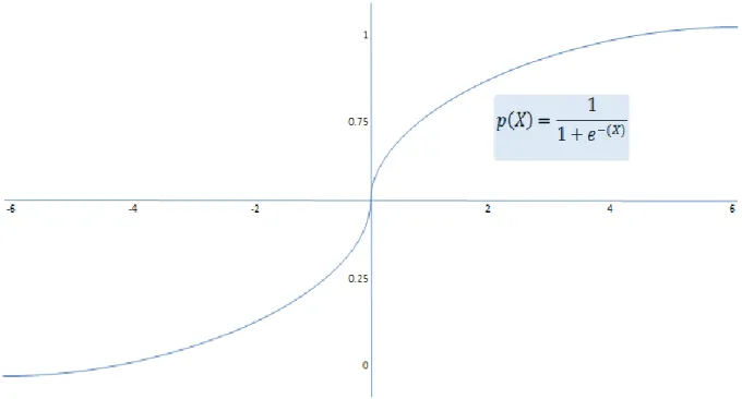
Logistic regression (LR) is a widely used model during the development period of credit scoring models. The reason for this is that the target variables in the credit scoring model are binary. Logistic regression uses the maximum likelihood estimation process (Anderson, 2007).
This process;
(1) transforming dependent variables into a logarithmic function, (2) which coefficients should be,
(3) the determination of coefficient changes and the maximization of the logarithmic likelihood.
ln (𝑝(𝐺𝑜𝑜𝑑)
1 − 𝑝(𝐺𝑜𝑜𝑑)) = 𝑏0+ 𝑏1𝑥1+ 𝑏2𝑏2 + ⋯ + 𝑏𝑘𝑏𝑘 + 𝑒 (𝟏)
The assumptions required to use logistic regression; 1. categorical target variable,
2. linear relationship in logarithmic odds functions,
3. Independent error term,
4. unrelated estimators, 5. the appropriate variables.
Today, credit scoring models are developed and logistic regression is accepted as the most important method. The reasons for this are;
1. design of binary outputs for finalization,
2. the probability of the results remaining between 0 and 1,
3. is to be able to make highly accurate probability estimates with the given information.
Compared with logistic regression, discriminant analysis and linear regression methods, it has the following advantages;
1. Logistic regression requires no assumption of normal distribution of
arguments.
2. Logistic regression can work well if there are large differences between group
sizes.
Figure 1. Standard Logistics Regression chart 2.2.2 Random Forest
Random forests or random decision forests are a community learning method for working classifications, regression and other tasks by creating a large number of decision trees at the time of the training and by creating a class (classifying) mode or average estimation (regression) of classes. Unstable decision forests correct the habit of over-fitting decision trees to the educational setting.
The first algorithm for random decision forests was created by Tin Kam Ho using the random subspace method, which is a way of applying a "stochastic discrimination" approach to the classification proposed by Eugene Kleinberg in Ho's formulation. The Random Forest (RF) is a community classifier that uses the paging mechanism. RF consists of a series of CART classifiers. At each node of a tree, only a small subset of features is selected for the partition; this allows the algorithm to quickly classify for high-dimensional data. The number of randomly selected features (try) should be determined in each section. The default value is secret (p) for the
classification of the number of properties of p. The separation criterion is the Gini index, as shown in Equation (1).
𝑔𝑖𝑛𝑖(𝑁) =1 2(∑ 𝑝(𝜔𝑗) 2 𝑗 ) (𝟐) 2.2.3 Decision Tree
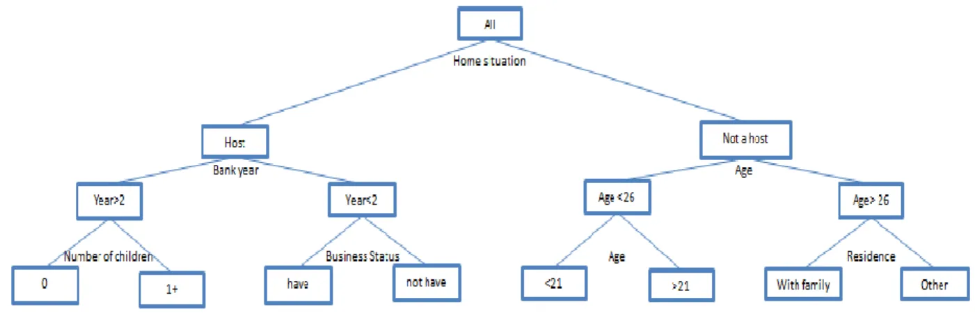
Decision tree (DT) is a graphical tool that shows the possible consequences of events to decision makers. Decision trees are also used in classification problems and
estimation problems. One of the advanced methods is data analysis. As an example of decision trees, the following graph can be given;
When this decision is considered downward, the top-tier age is defined as the basic needs of living with the family and becoming professional. Intermediate boxes; age, children, possession of the house, and intermediate nodes and bottom boxes are defined as end nodes. When the decision tree is over, the scores obtained from the finish node are used. A sample decision tree structure is shown in Figure 2.
Figure 2. A schematic representation of a sample decision tree structure Decision trees have several disadvantages and advantages over other techniques;
1. In the case of a set of rules, this technique can identify high or low risk categories that can be quickly and easily understood.
2. It is very simple to use with computer programs. The process ends with the
selection of the variables and the creation of the decision tree structure. But it is not a modeling process that has a lot of flexibility. There is not enough
information on how to make a lot of changes in the variables and affect the result.
3. The use of small data sets may lead to doubts about the reliability of the results. In order not to worry about the reliability of the model, it is necessary to work with large data sets.
4. It is quite simple to examine the results in simple decision trees. But it is rather difficult to examine the results when the decision tree structure is complicated (Anderson, 2007).
2.2.4 K-Nearest Neighbour Approach
The nearest neighbors technique is a standard, non-parametric approach to the
classification problem developed by Fix and Judges for the first time. This technique K - nearest neighbor approach was first applied by Chatterjee and Barcun, then by Henley and Hand. The logic on which this technique is based on choosing a distance in the application data space to measure how far apart any two applications are from each other. Sampled representation of past applicants is taken as standard. A new applicant is classified as good or bad on the basis of the well-bad ratio between close-up applicants (the nearest neighbor of the new application) in the sample (Thomas, 2002).
To implement this approach, three parameters are needed: the distance, how many reference counts (k) constitute the nearest neighbors set, and what should be the best rate of application for an application to be classified as good. Normally, if the
majority of the neighbors is good, the referral is classified as good. Otherwise the application is classified as bad. Define the average existing cost M, and the average loss profit K of rejecting good. If at least M / M + K of the nearest neighbors is good, a new reference is classified as good. If the proportion of neighbors who are likely to be good at a new application, this criterion will minimize the expected loss.
The choice of distance is very important. Fukanaga and Flick defined a general distance;
𝐴 (𝑥), is a p × p symmetric end positive matrix. If connected to x, A (x) is called local distance, if it is independent of x it is called global distance. The lack of local
distance often takes into account the characteristics of the unsuitable test set. For this reason, many researchers focus on global distance. The most detailed application of the nearest neighbors approaches in CS was done by Henley and Hand. With this technique, the focus is on a mixture of Euclidean length and good length, which best distinguishes evil. If w; the p-dimensional direction vector is the distance expression of Henley and Hand;
𝑑(𝑥1, 𝑥2) = {(𝑥1− 𝑥2)𝑇(𝐼 + 𝐷 𝑤𝑇)(𝑥1− 𝑥2)}12 (𝟒) Although the CS is not as frequently used as linear and logistic regression
approaches, the nearest neighbors have some important features for real applications. It is very easy to update the experiment set by dynamically adding new events and it can be easily removed from the sample when it is known that the addition is good or bad. Finding a good distance the first time is almost equivalent to creating a
scorecard with the regression technique. Thus, most practitioners prefer to stop at this point and use a traditional scorecard. When we compare it with the classification tree approach, the nearest neighbor approach does not produce a score for the future of each applicant. They identify a balance point for practitioners and they enable them to understand what the system actually does.
3.SUPPORT VECTOR MACHINE AND NEURAL NETWORK CREDIT SCORING CLASSIFICATION MODELS
3.1 Data Preprocessing
The R programming language was used to establish the models for classification in Credit Scores.
The German data set is used for modeling. The set consists of 21 columns (variable) and 1000 lines (data).
Variables- Existing account status, Month period, Credit history, Aim,Amount of
credit, Savings account / stock, Since then get a job, Installment rate, Personal status and sex, Other debtors / sureties, Place of residence, Estate, Age, Other plans of installments,Home, Number of existing loans in this bank,Job, The number of persons obliged to provide care,Phone, Foreign employee,Cost Matrix.
The extensive article attached to this article is given in Table 1.
Attribute Data Type Value Description
1 Existing account status qualitative A11 <0 A12 0 <= ... < 200 A13 >= 200
A14 no checking account
2 Month
period
numerical Duration in month
3 Credit history
qualitative A30 no credits taken/all credits paid back duly A31 all credits at this bank paid back duly A32 existing credits paid back duly till now A33 delay in paying off in the past
A34 critical account/other credits existing (not at this bank) 4 Aim qualitative A40 car (new)
A41 car (used)
A43 radio/television A44 domestic appliances A45 repairs
A46 education
A47 (vacation - does not exist?) A48 retraining A49 business A410 others 5 Amount of credit numerical 6 Savings account / stock qualitative A61 <100 A62 100 <= ... < 500 A63 500 <= ... < 1000 A64 >= 1000
A65 unknown/ no savings account 7 Since then
get a job
qualitative A71 unemployed A72 < 1 year A73 1 <= ... < 4 years A74 4 <= ... < 7 years A75 >= 7 years 8 Installment rate numerical 9 Personal status and sex
qualitative A91 male: divorced/separated
A92 female: divorced/separated/married A93 male: single
A94 male: married/widowed A95 female: single
debtors / sureties A102 co-applicant A103 guarantor 11 Place of residence numerical
12 Estate qualitative A121 real estate
A122 if not A121 : building society savings agreement/life insurance A123 if not A121/A122 : car or other, not in attribute 6
A124 unknown / no property
13 Age numerical
14 Other plans of
installments
qualitative A141 bank A142 stores A143 none 15 Home qualitative A151 rent
A152 own A153 for free 16 Number of
existing loans in this bank
numerical
17 Job qualitative A171 unemployed/ unskilled - non-resident A172 unskilled - resident
A173 skilled employee / official
A174 management/ self-employed/highly qualified employee/ officer 18 The number of persons obliged to provide care numerical
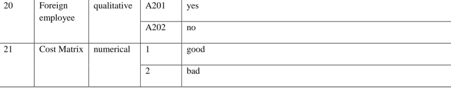
19 Phone qualitative A191 none
20 Foreign employee
qualitative A201 yes A202 no 21 Cost Matrix numerical 1 good
2 bad
Table 1. Information about the variables used in the Credit Scores
For modeling, Month period, Amount of credit, Installment rate , Place of residence,
Age, Number of existing loans in this bank, The number of persons obliged to provide care variables convert to numeric types.
3.1.1Analysis of Variables
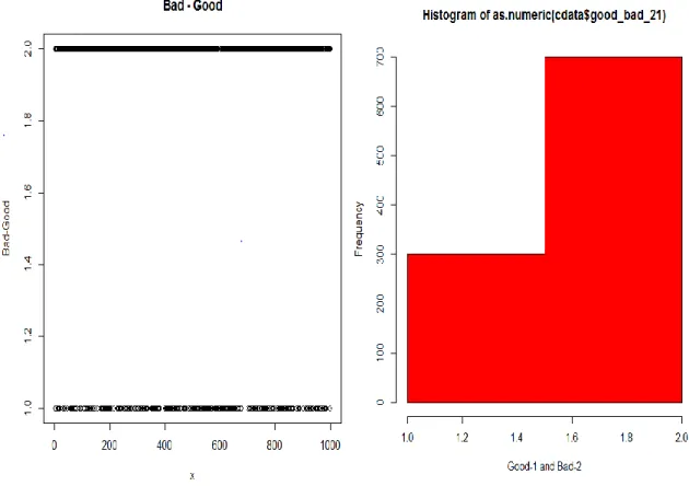
There are 300 bad and 700 good customers in the dataset. The customer analysis is described with charts using R graph, while the following values are calculated for each change.
Names- the value of the variable in the data set
Good- good customer count
Bad- bad customer count
Good_pct- good customer count by percentage
Bad_pct- bad customer count by percentage
Total-total customer count
Total_Pct- total customer count by percentage
Bad_Rate-Bad rate or response rate
grp_score-score for each group
WOE-Weight of Evidence for each group
IV-Information value for each group
Figure 3. Division of customer data for analysis and representation by histogram chart
Figure 4. Variable- Existing account status
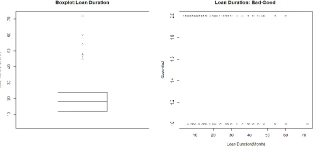
Table 2. Value ofVariable- Existing account status Variable- Month period :
Table 3. Value of Variable- Month period
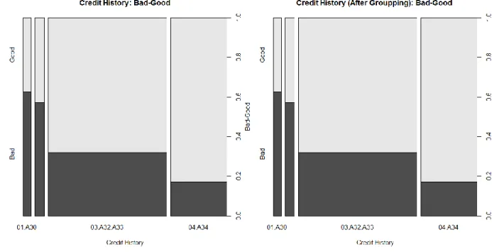
Figure 6. Variable- Credit History
Table 4. Value ofVariable- Credit History
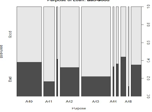
Figure 7. Variable- Aim of the loan
Table 5. Value ofVariable- Aim of the loan Variable- Amount of credit :
Figure 8. Variable- Amount of credit
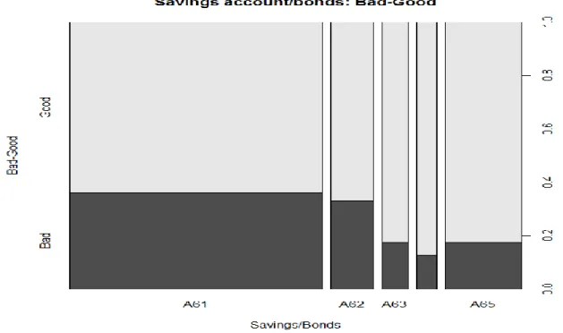
Table 6. Value of Variable- Amount of credit Variable- Savings account / stock :
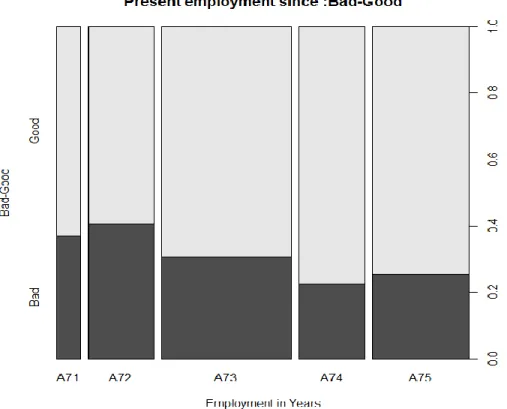
Table 7. Value ofVariable- Savings account / stock Variable- Since then get a job :
Figure 10. Variable- Since then get a job
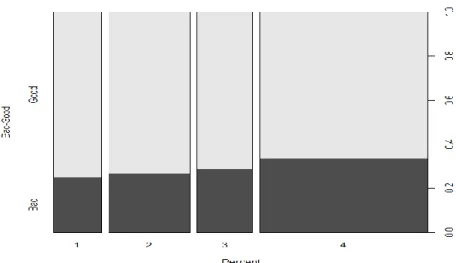
Table 8. Value ofVariable- Since then get a job Variable- Installment rate :
Figure 11. Variable- Installment rate
Table 9. Value ofVariable- Installment rate Variable- Personal status and sex :
Table 10. Value ofVariable- Personal status and sex
Variable- Other debtors / sureties :
Figure 13. Variable- Other debtors / sureties
Table 11. Value ofVariable- Other debtors / sureties Variable- Place of residence :
Figure 14. Variable- Place of residence
Table 12. Value ofVariable- Place of residence Variable- Estate :
Table 13. Value ofVariable- Estate Variable- Age :
Table 14. Value of Variable- Age Variable- Other plans of installments :
Figure 17. Variable- Other plans of installments
Table 15. Value ofVariable- Other plans of installments Variable- Home :
Figure 18. Variable- Home
Table 16. Value ofVariable- Home Variable- Number of existing loans in this bank :
Figure 19. Variable- Number of existing loans in this bank
Table 17. Value ofVariable- Number of existing loans in this bank Variable- Job :
Figure 20. Variable- Job
Table 18. Value of Variable- Job Variable- The number of persons obliged to provide care:
Figure 21. Variable-The number of persons obliged to provide care
Table 19. Value ofVariable- The number of persons obliged to provide care Variable-Telephone Number (Yes/No) :
Figure 22. Variable- Telephone Number (Yes/No)
Table 20. Value ofVariable- Telephone Number (Yes/No)
Figure 23. Variable- Foreign Employee(Yes/No)
Table 21. Value ofVariable- Foreign Employee(Yes/No)
3.1.2Partition of Data
After the data is analyzed, the partition is processed in the data set.
We can divide random samples with 50-50, 60-40, or 70-30 ratios for training (Model to be developed or trained), and Test (validation / retention pattern model can be tested according to population size). In the thesis, we will split the sample into 70-30. Three types of basic sampling strategy:
Random
Systematic
Simple random sampling is a sampling technique (example) when selecting a group of subjects to work with a larger group (population). Every individual is chosen purely by chance and every member of the population equals the chance of being included in the sample.
Select train sampling :
Select test sampling :
3.2 Support Vector Machine (SVM) Modeling 3.2.1 Support Vector Machine (SVM)
It is one of the most effective and simple methods used for classification. It is
possible to distinguish two groups by drawing a boundary between the two groups in a plane for classification. The place where this border can be drawn is that the two groups should be the farthest place to their members. Here SVM determines how this boundary is drawn.
In order to do this, two near and two parallel border lines are drawn on the two groups and these boundary lines are drawn closer together to produce a common boundary line. Take, for example, the following two groups:
Figure 24. Support Vector Machine algorithm
In this way, two groups are shown on a two-dimensional plane. It is possible to think of these planes and dimensions as properties. In other words, a feature extraction of each input that enters the system in a simple sense has resulted in a different point that shows every input in this two-dimensional plane. The classification of these points is the classification of inputs according to the properties that have been extracted.
It is possible to say the tolerance (offset) between the two classes above. The definition of each point in this plane can be made by the following notation:
𝐷 = {(𝑥𝑖, 𝑐𝑖)|𝑥𝑖 ∈ 𝑅𝑝, 𝑐𝑖 ∈ {−1,1}}
𝑖=1 𝑛
(𝟓)
It is possible to read the above formula as follows. For every x, c, the vector X is a point in our space and c is the value indicating that this point is -1 or +1. This set of points goes up to i = 1 'den n.
So this formula refers to the points of the previous form.
If we think that this formula is on an extreme plane (hyper plane). Every point in this formula:
can be expressed by the equation. Where w is the normal vector perpendicular to the hyper plane and x is the varying parameter of the point and b is the shear rate. It is possible to compare this equation to the equation for calc ax + b.
Again, according to the above equation b / || w || The value gives us the distance difference between the two groups. We have already given the tolerance (offset) value to this distance difference. In order to obtain the highest value of the distance according to this distance difference equation, 2 / || w || in the equation giving 3 straight values having the values 0, -1 and +1 shown in the first above, formula is used. That is, the distance between the lines is 2 units.
The two right equations obtained according to this equation are: 𝑤𝑥 − 𝑏 = −1 (𝟕)
𝑤𝑥 + 𝑏 = 1 (𝟖)
In fact, these equations are the result of finding the highest values obtained as a result of shifting the truths. It is also assumed that the problem is linearly separable with these equations.
As expected, it is not possible that the hyper plane between the two groups is one way. Here is an example of this situation:
Figure 25. In the SVM, it is not possible for the hyper plane to be unidirectional between the two groups
In case of two different hyper planes (extreme planes) as above, the SVM method takes the one with the greatest possible offset from these possibilities.
3.2.2 SVM - Vanilladot Kernel
Support Vector Machines are the perfect tool for classification, regression and
innovation detection. Svc, nu-saver (regression), no-Svc (classification) formulations with the well-known single class Svc (novelty) eps-saver, together with the kSVM, the classification formulations in native multi-species and the borderline SVM
formulations. In addition, KSVM supports confidence intervals and class probability output for regression.
KSVM Basic Model:
𝑘𝑠𝑣𝑚(𝑥, 𝑑𝑎𝑡𝑎, 𝑘𝑒𝑟𝑛𝑒𝑙)
𝑥 - A symbolic description of the model to follow. If you do not use a formula, x may be a matrix or vector containing training data, or a list of character vectors (for use with a character string kernel) or a kernel matrix of the class core matrix of training data. Note that regardless of whether the cut point is given in the form, it is always excluded.
𝑑𝑎𝑡𝑎 -is the data set containing the training data when using the formula. When no
parameter is given, the data are taken from the environment where `ksvm 'is called. 𝑘𝑒𝑟𝑛𝑒𝑙 - the core function used in prediction and training. This parameter can be set to any function of the core class that computes the inner product of the property field between the two vector arguments. Kernlab provides the most popular kernel
functions that can be used by setting the kernel parameter to the following strings: rbfdot - Radial Basis kernel "Gaussian"
polydot - Polynomial kernel vanilladot - Linear kernel
tanhdot - Hyperbolic tangent kernel laplacedot - Laplacian kernel
besseldot - Bessel kernel
splinedot- Spline kernel stringdot - String kernel
We have chosen the "VanillaDot Kernel" parameter as a kernel in designing our model.
𝑘𝑠𝑣𝑚(𝑥 = [𝑔𝑜𝑜𝑑_𝑏𝑎𝑑~], 𝑑𝑎𝑡𝑎 = [𝑡𝑟𝑎𝑖𝑛_𝑑𝑎𝑡𝑎_𝑠𝑒𝑡], 𝑘𝑒𝑟𝑛𝑒𝑙 = [𝑉𝑎𝑛𝑖𝑙𝑙𝑎𝑑𝑜𝑡]) 3.2.3 SVM - Gaussian RBF kernel
Radial base function kernel, also called RBF kernel, or Gaussian kernel is a cure in the form of a radial basis function (more specifically a Gaussian function). Gaussian kernel is probably the most used kernel functions. RBF kernel :
𝐾(𝑥, 𝑦) = 𝑒𝑥𝑝 {−‖𝑥 − 𝑦‖
2
2𝜕2 } (9)
Matches the input field to the infinite size property field. This feature is very flexible and can accommodate a wide variety of decision boundaries. The Gaussian kernel is often called the radial basis function (RBF). In some cases, it is parameterized
somewhat differently:
𝐾𝑅𝐵𝐹(𝑥, 𝑦) = 𝑒𝑥𝑝[−𝛾‖𝑥 − 𝑦‖2] (10)
The following function is used in our model in the Gauss Kernel model.
𝑘𝑠𝑣𝑚(𝑥 = [𝑔𝑜𝑜𝑑_𝑏𝑎𝑑~], 𝑑𝑎𝑡𝑎 = [𝑡𝑟𝑎𝑖𝑛_𝑑𝑎𝑡𝑎_𝑠𝑒𝑡], 𝑘𝑒𝑟𝑛𝑒𝑙 = [𝑅𝐵𝐹𝐷𝑜𝑡]) 3.3 Artificial Neural Network Modeling
3.3.1 Artificial Neural Network (ANN)
An artificial neural network is an information processing system arising from the imitation of the nerve cell and the nerve network by a computer. Artificial neural networks are interconnected, connected in parallel, distributed systems, each of which has its own information processing capability and memory. Artificial neural networks are systems of similar structure derived from artificial neurons in the human brain. Artificial neural networks are a mathematical model or measurement model developed based on biological neurons.
Artificial neural networks are artificial intelligence technologies that are multivariate and produce successful results when there is complex, mutual interaction between variables, or when a single set of solutions is not found.
Artificial neural networks have been developed through the mathematical modeling of human nervous systems and have certain assumptions (Fausett, 2004);
Information processing is through the elements called neurons.
The signal is propagated through the connections between the neurons.
Each connection has a certain weight and these weights are multiplied by the
signals.
Each neuron has an activation function that generates the output signal by
means of a formula.
Artificial neural networks are characterized by the following forms;
the connections between neurons,
(learning, teaching, algorithm) of the connections between the links,
activation formula (Fausett, 2004).
Figure 26. Systematic representation of Artificial Neural Network and biological neural network
Input
Entries are information from an outside world into an artificial neural cell. Entries in artificial neural networks are unprocessed data. Artificial neural network's
output according to input data. According to the weights of the inputs, the learning function is performed and the training phase is carried out.
Weights
Weights are the values that determine the effect of incoming information on the cell. The information enters the cell through the weights on the links and the weights show the relative strength (mathematical coefficient) of the values to be used as inputs in the artificial neural network. There are different weight values of all the connections that allow the inputs to be transmitted between cells within the artificial neural network. Thus, weights affect each entry of each processor
element. Weights can be variable or fixed. Activation function
The output value is obtained by using an activation formula summing the
weighted inputs. In most cases the output of the weighted input values from the activation process is between -1 and 1 or between 0 and 1. The activation
formulas used in most studies are shown in the following chart (Bigus, 1996). The sample activation functions are given in the following chart.
Activation function Mathematical Definition
Lineer 𝑓(𝑥) = 𝑥
Lojistik Sigmoid
𝑓(𝑥) = 1
1 + 𝑒𝑥𝑝(−𝑥)
Gaussion
𝑓(𝑥) = exp (− 𝑥
2
2𝜕2)
Output
Outputs are final process elements. The output is determined by the activation function. Each neuron sends its output as an input to another neuron. There is only one output value from a neuron. Artificial neural network output, solution of the problem. For example, loan appraisal, credit appraisal; positive or negative. Outputs such as input in artificial neural networks are composed of numerical values. +1 is positive, 0 is negative. It is the calculation of the objective output value of artificial neural networks.
3.3.2 Artificial Neural Networks Structure and Model Artificial Neural Networks have the following features:
Feedforward Neural Networks
Backpropagation Neural Networks
Multilayer Perceptron
Feedforward Neural Networks-In a Feedforward Neural Networks, the processor elements (PE) are generally divided into layers. The cells in each layer are fed only in the cells of the previous layer. In the forward 40-feed ANN, the cells are arranged in layers and the outputs of the cells are input as weights over the next layer. The entry layer conveys the information from outside the cells in the intermediate layer without any change. Information is processed in the middle and output layer to determine the network output. Signals are transmitted from the input layer to the output layer
through one-way connections. When the PEs establish a connection from one layer to another layer, there are no connections within the same layer. Examples of advanced networking include Multi Layer Perceptron (MLP) and Linear Vector Quantization (LVQ) networks (Alavala, 2002).
Feedback Neural Networks - There are dynamic memories of this kind of neural networks, and one output reflects both that input and the previous input. Therefore, they are used especially in forecasting applications. These networks have been quite
successful in predicting various types of problems. As an example of these networks; Hopfield, Self Organizing Map (SOM), Elman and Jordan networks (Alavala, 2002). Multilayer Perceptron- Multilayer sensor artificial neural networks are one of the most used neural network models in engineering applications.Many layered sensors (perceptron model, consisting of one input, one or more intermediate and one output layer).All the processing elements in a layer depend on all the processing elements in a top layer.The information flow is forward and there is no feedback.For this reason, it is called as a feedforward neural network model.
The following function has been used to train the Neural Network:
𝑛𝑛𝑒𝑡(𝑓𝑜𝑟𝑚𝑢𝑙𝑎, 𝑑𝑎𝑡𝑎, 𝑠𝑖𝑧𝑒, 𝑚𝑎𝑥𝑖𝑡, 𝑑𝑒𝑐𝑎𝑦, 𝑙𝑖𝑛𝑜𝑢𝑡, 𝑡𝑟𝑎𝑐𝑒) (11)
formula- A formula of the form class : 𝑥1 + 𝑥2 + ...
data- The data frame to be taken first of the variables specified in the formula
size- number of units in the hidden layer.
maxit-maximum number of iterations.
decay- parameter for weight decay.
linout-switch for linear output units.
trace-switch for tracing optimization.
3.4 Scoring Model with Support Vector Machine and Artificial Neural Network 3.4.1 Scoring with SVM - Vanilladot Kernel Model
We use the ksvm function and the kernel parameter Vanilladot function in the study. We apply this model on the test data.
With the first once predict function, we get a score for the test data, then we look at how well these scores match our target data with the prediction function capability. Then the performance evaluation of the model is done. The performance evaluation is calculated according to the output values.
Figure 27. SVM - Vanilladot Kernel Model ROC Curve The ROC curve (A Receiver Operating Characteristic Curve) shows the performances of the two cluster classifiers at the possible rung intervals. Ideal classifiers are collected on the left and top of the graph under the points where the curve has a value of 1.0. Random classifiers are successful at around 0.5 (classifiers in the area below 0.5 can be developed).
ROC curve classifiers are recommended for benchmarking, not just the arbitrarily chosen decision step, but the performance in all possible decision steps. The ROC curve is used to select the optimum step decision. This step (equal to the wrong classification ratio in both classes) can be used automatically in the step confidence setting.
Classification
Observation Prediction
Good Bad Rate
Good 183 38 82%
Bad 27 52 65%
Average Rate 70% 30% 78%
Table 22. Outcome from classification made with SVM-VanillaDot Kernel model As we have seen from the classification chart, the number of well-estimated
customers (183) is really good, 82% and the number of poorly estimated customers actually good is 38. In reality, the ratio of badly estimated customers (52) is 65%, and in reality, if it is bad, the number of customers estimated to be good is 27. According to the SVM-Vanilladot Kernel model, the prediction success is 78% for good and bad customers.
In the model, the support vector number is 399 and the training error is 0.225714 And finally, the performance of the model was evaluated by three important Model Evaluation Error Criteria.
Model Evaluation Error
Metrics
Performance Metrics
AUROC (AUC – ROC) 81.50
KS (Kolmogorov Smirnov) 46.82
Gini (Gini Coefficient) 63.02
Table 23. Outcome from the evaluation of SVM-VanillaDot Kernel model with Model Evaluation Error Criteria
We use the Support Vector Machine classification method to examine a second scoring model. The same KSVM function was used to set up our model, but unlike the Vanilladot model, RBFDot (Gaussian RBF) was chosen as the kernel parameter. As with the VanillaDot model, new functions are estimated for customers with forecasting functions.
Now let's look at the ROC Curve of this model.
Figure 28. SVM - Gaussian RBFModel ROC Curve
The predicted maximum value (1.93) was the minimum value (-1.61) as seen from the ROC curve.
SVM- Gaussian RBF Kernel model shows the results of classifications realized in the following chart.
Classification
Observation Prediction
Good Bad Rate
Good 199 60 76%
Bad 11 30 73%
Average Rate 70% 30% 76%
Table 24. Outcome from classification made with SVM- Gaussian RBF Kernel model
The above table shows that the number of well-estimated customers is 199 and the rate is 76%. The number of customers is 30 and the ratio is 73%. The number of customers who are really bad and who are good at the estimate is 11, Our model's prediction success rate is 76%.
In the SVM-Gaussian model, support vector number 457 and training error 0.2 were observed.
Performance evaluation of the Scoring Model was measured as follows.
Model Evaluation
Error Metrics
Performance Metrics
AUROC (AUC – ROC) 72.89
KS (Kolmogorov Smirnov) 38.42
Table 25. Outcome from the evaluation of SVM- Gaussian RBF Kernel model with Model Evaluation Error Criteria
3.4.3 Scoring with Artificial Neural Networks Model
Neural Networks, NeuralNetTools, e1071 libraries are used in modeling of Artificial Neural Networks with R programming language.
First, the Train and Test data are normalized by the normalize function.
Normalize<- function (x)
Return( (x-min (x)) / (max(x)-min(x)))
The model uses a multi-layer sensor network structure, that is, it has a feedforward structure consisting of three layers of input, neural network middle and output layers. The model of the network is as follows:
Figure 29.ANN model architecture
As you can see from the picture, 24 input variables are included in the neural network, these inputs are passed to the next layer and the number of inputs in this
intermediate layer is reduced to 20.And the output layer, which is our last layer, consists of 1 variable.The connection weights of the nerve cells are 521.The nnet function is selected for training of neural networks.
And the parameters of this function are given in the appropriate input Table 26.
Parametre Value
formula V25 ~ V1+V2+V3+…+V24
data train_nn (normalize olunmuş
train veriler) size 20 maxit 10000 decay 0.01 linout F trace F
Table 26. Parameter inputs for the ANN training function
The result table of the Artificial Neural Network model configured for classification in scoring model:
Classification
Observation Prediction
Good Bad Rate
Good 162 56 54%
Bad 46 36 12%
Average Rate 69% 31% 66%
The number of well-anticipated customers is 162 and the ratio is 54%. The number of malicious customers is 36 and the ratio is 12%. The estimated number of clients coming out badly is calculated as 56. And the predictive success of the model is 66% -dir.
The performance curve and values of the model are shown below.
Figure 30. ANN Model ROC Curve
Model Evaluation
Error Metrics
Performance Metrics
AUROC (AUC – ROC) 74.60
KS (Kolmogorov Smirnov)
43.61
Gini (Gini Coefficient) 49.30
Table 28. Outcome from the evaluation of ANN model with Model Evaluation Error Criteria
CONCLUSION
The size and importance of the banking sector are closely monitored by governments and supervisory agencies. The most important risk that affects the banking sector is the concept of credit risk. Credit risk can be described as the risk that arises if the credited creditor is not paid. The banks try to make sure that the customers they give credit are well known and that they can repay the loans they give. But nowadays the number of people who use credit from banks reaches to millions, making trusting and customer-based lending process very difficult. Techniques called credit scoring
techniques and measuring whether or not to give credit to customers using customer information are now widely used between banks today.
Credit scoring is a technique that uses the customer information to decide whether to give credit to customers who apply for credit. With credit scoring methods, it should be possible to lower the percentage of credit customers who will face difficulties in repayment when choosing lenders to receive higher rates of success and fail to pay back loans. Using statistical and non-statistical methods, the customers pass through the credit scoring and a score is formed in the bank's hands with the 2 customer information they hold.
Some banks in Azerbaijan now use scoring models. In particular, scoring models play an indispensable role in providing consumer loans. Because the information required to give consumer loans in Azerbaijan is almost transparent and the scoring model makes the analysis more accurate and gives more realistic results. There are problems with business loans. It is difficult to assess the financial account deficiency in some Azerbaijani businesses. However, if banks invest in this direction, scoring models can be created for such businesses. Right now, the lack of competition in the credit
market is creating wider income sources for banks, and even a decision made by a bad credit scoring model is better than the credit decisions made by some credit analysts at the bank. Within a few years, banks will have to pay more attention to credit risks - because the banks that do not manage the risks will be the least profitable and the closest banks to the bankruptcy.
Data analysis in the day, that is to say, the examination of the data into meaningful information is seen as the key to success for many sectors. Credit scoring is one of the newest applications used in the banking sector in our country for this purpose. As
credit scoring can be used for many purposes in banking applications, only
application scoring is covered in this study. Models have been prepared to estimate whether customers applying for loans are at risk and whether they apply. With these techniques, customers are classified as good-bad.
In this study, the data of credit customers of a bank were analyzed by some credit scoring techniques. Support Vector Machine and Artificial Neural Network were used in non-statistical techniques.
The Support Vector Machine algorithm uses the ksvm function, and the function has two different functions as kernel parameters: Vanilladot Kernel and Gaussian RBF Kernel. In the SVM Vanilladot Kernel model, 399 support vectors were used and training error was 0.225714,in the SVM Gaussian RBF Kernel model, 457 support vectors are used and the training error is equal to 0.2.
As the Artificial Neural Network, multilayer feed-forward network is preferred, and the connection weights of the neural networks are specified as 521. The first inputs are 21 variables, 20 of which are passed to the middle layer and 1 output (bad or good) is obtained.
The goal of the study is to compare some of the techniques that can be used for credit scoring by applying the same example.
The first applied SVM is the Vanilladot Kernel Model. The model showed 78% accuracy in determining the good and bad customers. The performance indicators AUROC = 72.89, KS = 38.42, Gini = 46.02.
Secondly SVM - Gaussian RBF Kernel Model was applied. Modeling give bad results in evaluating performance, but the accuracy of prediction indicators is 76%. The final implementation technique is Artificial Neural Networks Model. The
predictor of the model is 66%, performance values are AUROC = 74.60, KS = 43.61, Gini = 49.30.
It is the model SVM - Vanilladot Kernel, which has the best performance estimation among the models for this study and which has the best performance measures at the same time. The SVM - Vanilladot kernel is the SVM - Gaussian RBF kernel and ANN, respectively, which make good estimation after.
Order of the good customers with the highest classification accuracy is; SVM - Gaussian RBF kernel, SVM - Vanilladot Kernel, ANN.
Model ranking with the worst customers with the highest classification success; SVM - VanillaDot Kernel, ANN and SVM - Gaussian RBF kernel.
If we sort by performance evaluation: SVM - VanillaDot Kernel, YSA and SVM - Gaussian RBF kernel.
Reference
1. Ahmad Ghodselahi(2011) A Hybrid Support Vector Machine Ensemble
Model for Credit Scoring, Department of Information Technology Management Tarbiat Modares University Tehran, Iran;
2. Alavala, C.R. (2003). Fuzzy logic and neural Networks: Basic concept & appliations, New Age International Publisher;
3. Anderson, R. (2007). The Credit Scoring Toolkit, Oxford University Press,
4. Arminger, G., Enache D. and Bone T., (1997), “Analyzing Credit Risk
Data: A Comparison of Logistic Discrimination, Classification, Tree Analysis, and Feedforward Networks”, Computational Statistics;
5. Bigus, J. P. (1996). Data Mining with Neural, Networks McGraw-Hill.
6. Brown, I., and Mues, C. An experimental comparison of classification
algorithms for imbalanced credit scoring data sets. Expert Systems with Applications;
7. Cristianini, N., and Shawe-Taylor, J. ( 2000)An Introduction to Support
Vector Machines and Other Kernel-based Learning Methods. Cambridge University Press;
8. de Souza, C. R.( 2010) Kernel functions for machine learning applications,
March;
9. Dr. Ir. Tony Van Gestel(1), Bart Baesens(2), Dr. Ir. Joao Garcia(1), Peter Van Dijcke(3), A Support Vector Machine Approach to Credit Scoring;
10.Fausett, L., “Fundamentals of Neural Networks : Architectures, Algorithms
and applications”;
11.Finlay ,S.,(2012) Credit Scoring, Response Modeling, and Insurance
Rating: A Practical Guide to Forecasting Consumer Behavior. Palgrave Macmillan;
12.Ha Van Sang1* , Nguyen Ha Nam2 , Nguyen Duc Nhan3(2016) A Novel
Credit Scoring Prediction Model based on Feature Selection Approach and Parallel Random Forest, Indian Journal of Science and Technology;
13.https://archive.ics.uci.edu/ml/datasets/statlog+(german+credit+data)
14.http://banker.az/
15.https://www.cbar.az/
16.http://cran.r-project.org/
18. https://www.r-bloggers.com/using-neural-networks-for-credit-scoring-a-simple-example/
19.https://www.rdocumentation.org/
20.Lee, T. S., Chiu, C. C., Chou, Y. C. and Lu C. J. (2006). Mining the customer credit using classification and regression tree and multivariate adaptive regression splines;
21.Lewis, E.M., (1992), An Introduction to Credit Scoring, Athena Press, San
Rafael, Thomas;
22.Platt, J. C. Fast(1999) training of support vector machines using sequential minimal optimization. In Advances in kernel methods, MIT press;
23.Sunil Bhatia, Pratik Sharma, Rohit Burman , Santosh Hazar, Rupali
Hande(2017) , Mumbai University, International Journal of Computer Applications
24.Sustersic, M., Mramor, D. and Zupan J. (2009). Consumer credit scoring
models with limited data. Experts Sysems with Application,
25.Thomas, L.C., Edelman, D.B. and Crook, J.N. (2002). Credit Scoring and
Its Applications, Society For Industrial and Applied Mathematics;
26.Williams(2008), C. Support Vector Machines. School of Informatics,