2011-7
is
s
Na
ti
on
al
B
an
k
W
or
ki
ng
P
ap
er
s
Sectoral Inflation Dynamics, Idiosyncratic Shocks and
Monetary Policy
The views expressed in this paper are those of the author(s) and do not necessarily represent those of the Swiss National Bank. Working Papers describe research in progress. Their aim is to elicit comments and to further debate.
Copyright ©
The Swiss National Bank (SNB) respects all third-party rights, in particular rights relating to works protected by copyright (information or data, wordings and depictions, to the extent that these are of an individual character).
SNB publications containing a reference to a copyright (© Swiss National Bank/SNB, Zurich/year, or similar) may, under copyright law, only be used (reproduced, used via the internet, etc.) for non-commercial purposes and provided that the source is mentioned. Their use for commercial purposes is only permitted with the prior express consent of the SNB.
General information and data published without reference to a copyright may be used without mentioning the source.
To the extent that the information and data clearly derive from outside sources, the users of such information and data are obliged to respect any existing copyrights and to obtain the right of use from the relevant outside source themselves.
Limitation of liability
The SNB accepts no responsibility for any information it provides. Under no circumstances will it accept any liability for losses or damage which may result from the use of such information. This limitation of liability applies, in particular, to the topicality, accuracy, validity and availability of the information.
Sectoral Inflation Dynamics, Idiosyncratic Shocks and
Monetary Policy
∗
Daniel Kaufmann
†and Sarah Lein
‡26 April, 2011
Abstract
This paper disentangles fluctuations in disaggregate prices into macroeconomic and idiosyncratic components using a factor-augmented vector autoregression (FAVAR) in order to shed light on sectoral inflation dynamics in Switzerland. We find that disaggregated prices react only slowly to monetary policy and other macroeconomic shocks, but relatively quickly to idiosyncratic shocks. We document that there is a large heterogeneity across sectors in the reaction to monetary policy shocks and show that sectors with larger volatility of idiosyncratic shocks react more readily to monetary policy. This finding stands in contrast to the rational inattention model of price setting. We also find that sectors, which change prices infrequently, react less strongly but if they do change their prices, they adjust them by a large amount. This suggests that the source of sluggish response to aggregate shocks is heterogeneity in menu costs rather than rational inattention. Furthermore, even though prices respond with a significant delay to identified monetary policy shocks, we find no evidence of a price puzzle on average. For single sectors, however, we still find a hump-shaped response which can partially be explained by the fact that, by law, rents are tied to interest rates in Switzerland. JEL classification: E31, E4, E5, C3
Keywords: monetary policy transmission, idiosyncratic shocks, rational inattention, heterogeneity in price setting, cost channel, price puzzle
∗We thank Gregor B¨aurle, Marc Giannoni, Matthias Lutz, Klaus Neusser, Barbara Rudolf, Frank Schmid, Peter
Tillmann and Mathias Zurlinden, an anonymous referee for the SNB working paper series and participants at the YSEM meeting in Bern and the SNB’s Brown Bag seminar for helpful comments and suggestions. Andreas Bachmann and Andrea Schnell provided excellent research assistance. The views expressed in this paper are those of the authors and not necessarily those of the Swiss National Bank.
†Swiss National Bank, B¨orsenstrasse 15, P.O. Box, CH-8022 Zurich, Switzerland, E-mail: daniel.kaufmann@snb.ch
1
Introduction
Recent evidence on micro price adjustment shows some challenging effects for the theoretical literature on monetary non-neutrality. Although prices are only infrequently adjusted at the micro level, the degree of price stickiness is too low to explain the persistence of aggregate inflation rates. Hence, there is an inconsistency between the micro and the macro facts on prices, which calls for theoretical models that can bridge this gap.
The literature has taken different directions for modelling this feature of price-setting behaviour. Mackowiak and Wiederholt (2009) argue that if idiosyncratic shocks are large relative to macroeconomic shocks it may be rational for individual firms to direct most of their attention to the idiosyncratic shocks. As a consequence of this rational inattention, macroeconomic shocks are incorporated only slowly into prices. Another strand of the literature emphasises the macroeconomic implications of differences in price-setting behaviour across firms or sectors. Various authors have argued that monetary policy may have different welfare implications depending on whether or not price-setting behaviour is characterised by cross-sectional heterogeneity in the frequency of price changes. Carvalho (2006) stresses that heterogeneity in price stickiness and thus monetary policy responsiveness across sectors is important because it leads to more persistent real effects of monetary policy. Nakamura and Steinsson (2010) make a similar argument in a menu-cost model. Barsky et al. (2007) show that, even if most prices are flexible, a small durable goods sector with sticky prices may be sufficient to make output and inflation react to monetary policy as if most prices were sticky. Thus, the degree of monetary policy effectiveness depends disproportionately on the sectors with larger rigidities (Aoki, 2001).
The goal of this paper is therefore to confront these theoretical predictions with empirical evidence. Using a factor-augmented vector autoregression (FAVAR) and disaggregated index items from Switzerland’s consumer price index (CPI), we disentangle idiosyncratic and macroeconomic shocks using the framework presented in Boivin et al. (2009). We then calculate sectoral price responses to a monetary policy shock and identify the sectors with more sluggish price responses where inflation stabilisation may be more important.
The results imply that disaggregated prices react only slowly to monetary policy and other macroeconomic shocks, but relatively quickly to idiosyncratic shocks. Furthermore, there is a lot of heterogeneity in these reactions across sectors. This finding corroborates recent evidence for the US (Boivin et al., 2009; Mackowiak et al., 2009) and the UK (Mumtaz et al., 2009) and is in line with predictions from both strands of the theoretical literature.
Focusing on the sources of the cross-sectional variation of price responses to a monetary policy shock, we find that the response of firms to a monetary policy shock increases with the volatility of the idiosyncratic shocks. Our estimates suggest that 70% of the cross-sectional differences in price responses can be explained by the degree of volatility of idiosyncratic shocks. Controlling for the volatility of macroeconomic shocks does not changes the result. This is not consistent with the rational inattention model of price setting, which implies that firms facing volatile idiosyncratic shocks will pay less attention to macroeconomic shocks. In addition, we find that the extent of the response to a monetary policy shock is related to the degree of price stickiness. The price response to a monetary policy shock tends to be sluggish in those sectors with infrequent but large price adjustments. This is consistent with the idea that cross-sectional differences in price adjustment costs, or menu costs, explain differing price responses to a monetary policy shock.
We then use the results from the FAVAR to examine the pattern of responses of disaggregate inflation rates to monetary policy shocks. The results show that prices respond to a monetary policy tightening with a lag of about 6 to 7 quarters. In contrast to traditional VAR analysis, the response of the CPI to a monetary policy shock displays no price puzzle, i.e., no temporary increase in inflation after a monetary policy tightening (cf. Christiano et al., 1999). This is due to the fact that the FAVAR incorporates more information than VARs, where economic activity is proxied by a small number of variables only.
Although we find no price puzzle at the aggregate level, there is a substantial amount of heterogeneity in the responses of disaggregate prices. Therefore, we look at the responses of individual CPI items aggregated to sectors such as goods or services separately. We find that durable goods react with a significant delay of 12 quarters while semi-durable and non-durable goods prices react much faster. We find a rather slow response for services. Rents, especially, increase significantly after a monetary policy tightening, which is not surprising, given the fact that rents are linked to the short-term mortgage rate in Switzerland, so that monetary policy tightening is likely to lead to higher rents. We also find a hump-shaped response of prices for durable goods and services excluding rents. We argue that this may be due to the cost channel of monetary policy, which is more important in the case of larger inventory holdings (durable goods) and real wage rigidities (services).
The remainder of this paper is structured as follows. Section 2 presents the data and the FAVAR methodology. Section 3 discusses our results, and Section 4 concludes.
2
Data and methodology
We follow Boivin et al. (2009) and use a FAVAR to analyse disaggregate inflation dynamics. Compared to a standard VAR, the advantage of the FAVAR developed in Bernanke et al. (2005) is that it exploits the information content of a considerably larger set of macroeconomic variables. In addition, the framework makes it possible to decompose the fluctuations of disaggregate price series into a common and an idiosyncratic component, which can be used to assess the relative importance of macroeconomic and idiosyncratic factors in explaining disaggregate price fluctuations.
Factor analysis allows us to summarise the information from a large number of time series, using a relatively small set of estimated factors. Let us assume that the Swiss economy is affected by a vector Ct of common components. One of the common components is the 3M Libor as a
measure of the monetary policy instrument (Rt), which can be observed.1 The remaining common
components are denoted by aK×1 vector of unobserved factorsFt. These unobserved factors may
reflect general economic conditions such as real economic activity, the general rate of inflation, and asset prices. LetFt andRtfollow the transition equation
Ct=Φ(L)Ct−1+υt , (1)
where Ct = [Ft Rt] and Φ(L) is a conformable lag polynomial. The error term υt is an
i.i.d. random vector with mean zero, andtis the time index t= 1, ..., T. The transition equation
represents a VAR in the unobserved factors and the 3M Libor.
Since we do not observe Ft we extract it from a large data set of economic time series. The
number of these series is denoted byN, which should be large relative toKandT. Let the series
be denoted by aN×1 vectorXtthat is related to the common factors according to the observation
equation
Xt=ΛCt+et , (2)
whereΛ is aN×(K+ 1) matrix of factor loadings. The principal component estimation which
is applied to extract the factors Ft allows for some cross-correlation in the error term (et) that
vanishes asN goes to infinity (cf. Stock and Watson, 2002). Once the factors have been extracted,
the factor loadings can be estimated by OLS. Equations (1) and (2) represent a dynamic factor model where – conditional on Rt – the variables in Xt are noisy measures of the underlying
1The Swiss National Bank sets an operational target range for its chosen reference interest rate, the 3M
unobserved factorsFt. Via the transition equation (1), the unobserved componentsFtcan always
include arbitrary lags ofXteven thoughXtdepends only on the current and not on lagged values
ofFt.
The matrixXt consists of a panel of quarterly data from Q1 1978 to Q3 2008. The data set
includes 142 macroeconomic time series and the growth rates of 151 index items from the Swiss CPI.2 An index item is defined as the price index at the lowest level of disaggregation. We refer
to the growth rates of these indices as disaggregate inflation. We have aggregated some of the individual CPI items to a higher level in order to obtain consistent price indices over the whole sample period. In addition, we had to exclude some of the items underlying the CPI today, due to data availability restrictions. Also, we removed administered prices since it is not clear whether they are affected by monetary policy or not. The resulting data set includes 80% of the CPI at average weights.3
From the data set we extract the factors as suggested by Boivin et al. (2009). A recursive procedure is applied to imposeRt as a common component on the data setXt and to obtain a
consistent estimate ofFt. Initially, we obtain the firstK principal components fromXt, denoted
byF0
t. We then estimateˆλ
0
Rby regressingXt onF0t andRt. Next, we subtract the factorRtby
calculatingX˜0t =Xt−ˆλ
0
RRt. Then, we estimateF1t as the firstK principal components ofX˜
0
t.
The procedure is repeated several times to obtain the final estimate ofFt.
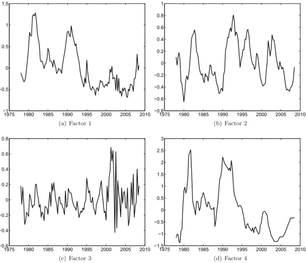
The question as to how many factors we should extract from the data can be answered by the test suggested in Bai and Ng (2002). Their test suggests that three factors summarise the information content ofXtwell. Therefore, we setK= 3 and end up with four common components
(cf. Figure 1).4 All in all, the factors explain 34% of the variation inX
ton average. The median
R2 is higher at 55%.
It is worth noting that we do not identify the factors as specific economic concepts. Nevertheless, we can examine the size of the corresponding factor loadings or the correlation of the factors with the underlying time series to find out which part of the economy a factor is most closely related to. Table 7 of the Appendix lists the 15 largest loadings (in absolute terms) of the time series inXtincluded in each of the four factors. The first factor appears to be mostly
related to price series such that it may capture general inflation dynamics. The second factor is
2A list of the series is provided in the Appendix in Tables4and5. The series have been seasonally adjusted
and transformed to induce stationarity, if necessary.
3The average weights of various subaggregates of the CPI are given in Table6of the Appendix.
4AsBernanke et al.(2005) emphasise, the test does not answer the question of how many factors we should
include in the VAR to capture the relevant dynamics but only how many factors capture the information in the data set well. However, we have experimented with more factors and the results remain qualitatively the same.
Figure 1: Estimated factors 1975 1980 1985 1990 1995 2000 2005 2010 −1 −0.5 0 0.5 1 1.5 (a) Factor 1 1975 1980 1985 1990 1995 2000 2005 2010 −0.8 −0.6 −0.4 −0.2 0 0.2 0.4 0.6 0.8 1 (b) Factor 2 1975 1980 1985 1990 1995 2000 2005 2010 −0.6 −0.4 −0.2 0 0.2 0.4 0.6 0.8 (c) Factor 3 1975 1980 1985 1990 1995 2000 2005 2010 −1.5 −1 −0.5 0 0.5 1 1.5 2 2.5 3 (d) Factor 4
Notes: The figures display the estimated factors used in the FAVAR. Factor 1 is mostly related to prices, Factor 2 to (inverse) real activity, and Factor 3 to (foreign) goods prices with sales. Factor 4 shows the normalised 3M Libor.
mostly driven by data covering the real economy, such as orders, sales or business sentiment. Most of the factor loadings are negative such that the factor is probably negatively correlated with real activity. It could therefore serve as an inverse real activity measure. This is supported by the fact that the factor is strongly correlated with one of the output gap measures that is calculated regularly by the Swiss National Bank (contemporaneous: -0.67; two quarters ahead: -0.79; cf. Figure 8 in the Appendix). The third factor is driven by prices for clothing and footwear. This is probably due to the fact that these prices are very volatile and highly seasonal. The Swiss Federal Statistical Office started to collect end-of-season sales prices in May 2000. This resulted in a higher volatility of this factor even though the series have been seasonally adjusted. By construction, the fourth factor is the 3M Libor. It is related to various interest rate spreads, the mortgage rate but also to technical capacities and various price series. Alternatively, instead of looking at the size of the factor loadings, one can compare correlations of the factors with the macroeconomic time series inXt. Table 8 of the Appendix shows the 15 largest correlation coefficients in absolute
terms. The correlations would lead to the same interpretation of the factors.
The observation equation can be used to disentangle the idiosyncratic from macroeconomic fluctuations for each CPI index item included inXt. Equation (2) implies that the decomposition
for each price series is of the form
πit=λiCt+eit , (3)
where πit denotes the log quarterly change of CPI index item i at time t, λi is the row vector
of factor loadings for itemi, andeit is the item-specific error term, which captures idiosyncratic
inflation dynamics that are not attributed to macroeconomic fluctuations. This allows us to relate every CPI index item to the transition equation, and therefore we can calculate the response of the disaggregated price series to various shock measures. We labelλiCt as the common component
of inflation andeitthe idiosyncratic component henceforth.
3
Results
The results are presented in the following order. Section 3.1 focuses on the common and idiosyncratic components of the CPI index items. First, we analyse their relative contribution for disaggregate inflation in a descriptive manner. Then, we calculate impulse responses in the FAVAR framework to obtain an estimate of the sluggishness of price responses and we relate differences in responses to monetary policy shocks to differences in the volatility and persistence
Table 1: Volatility and persistence of quarterly inflation rates (1) (2) (3) (4) (5) (6) (7) sd(πit) sd(λiCt) sd(eit) R2 ρ(πit) ρ(λiCt) ρ(eit) Aggregate series CPI Total 0.29 0.21 0.20 0.52 0.86 0.92 -0.13 Goods 0.33 0.21 0.25 0.41 0.61 0.84 0.16 Services 0.26 0.22 0.15 0.69 0.89 0.93 0.55 Excl. oil 0.25 0.20 0.15 0.65 0.84 0.92 0.02 Excl. rents 0.29 0.19 0.22 0.42 0.68 0.91 -0.01 Disaggregated series CPI Average 0.69 0.29 0.61 0.29 0.42 0.84 0.01 Wght. average 0.50 0.23 0.43 0.30 0.44 0.67 0.13 Median 0.42 0.21 0.36 0.29 0.52 0.87 0.08 Min. 0.15 0.03 0.12 0.01 -0.69 0.29 -1.99 Max. 4.08 1.14 3.92 0.67 0.90 0.94 0.81 Std. 0.70 0.19 0.69 0.17 0.35 0.10 0.45
Notes: The table gives the standard deviation (in percent) and persistence (ρ) of inflation (πit), the common component (λiCt), and the idiosyncratic component (eit). TheR2gives the share of variation inπitexplained by
λiCt. Weighted average statistics are calculated using average CPI weights over the whole sample period.
of inflation and heterogeneity in price-setting behaviour. Section 3.2 then analyses the monetary policy transmission in more detail. We show that, on average, prices react with a considerable lag, and examine why we find a price puzzle in some sectors but not in others.
3.1
Idiosyncratic vs. macroeconomic shocks
3.1.1 Descriptive analysis
Table 1 shows some descriptive statistics for aggregate CPI measures (upper panel) and disaggregate items of the CPI (lower panel). In Column (1), we report the standard deviation for the aggregate and disaggregate inflation rates (πit). Column (2) shows the standard deviation
for the estimated common components (λiCt) and Column (3) for the idiosyncratic component
(eit). Column (4) reportsR2 statistics measuring the fraction of inflation variation explained by
the common component.
The standard deviation of aggregate inflation amounts to 0.29, which is slightly higher than what is found by Boivin et al. (2009) for the US (0.24). The volatility for goods (0.33) is slightly higher than the volatility for services (0.26). A large share of the volatility in aggregate measures of inflation is due to fluctuations in the four common components. The R2 indicates
that macroeconomic fluctuations explain 52% of aggregate CPI inflation variation, and even 69% of the inflation variation for services. Relative to the rather small number of factors we use these
figures appear to be substantial.5 For the CPI excluding rents the variation attributed to the
common component is somewhat lower (0.42) than for the total CPI. This implies that rents are quite strongly driven by common component shocks. This may be due to the fact that rents are linked to mortgage rates in Switzerland and thus may be related to the 3M Libor. The opposite applies when excluding oil prices. Then theR2is higher than for the overall CPI. It appears that
oil product prices are to a larger extent driven by idiosyncratic shocks which is intuitive since they primarily depend on fluctuations in crude oil spot prices.
Column (5) reports the degree of persistence for the original series and Columns (6) and (7) for the common component and the idiosyncratic component, respectively.6 For all subaggregates
the persistence of the common component is higher than the persistence of the idiosyncratic component. Idiosyncratic persistence for total CPI inflation is small (-0.13). For services, idiosyncratic shocks seem to be more persistent than for the other subaggregates. The persistence of the common component is close to unity for all subaggregates.
The lower panel in Table 1 shows the summary statistics of the 151 CPI index items. In line with previous studies, the average volatility of disaggregate inflation rates (0.69) is higher than the volatility of the aggregate CPI (0.29). Interestingly, the variation in the common component explains only about 29% of the variation of the disaggregated inflation rates on average.7 This
indicates that disaggregated prices are mainly driven by idiosyncratic shocks while aggregate CPI can be explained to a large extent (52%) by macroeconomic shocks. Turning to the degree of persistence, we find that the average persistence of disaggregated inflation (0.42) is lower than the persistence of aggregate inflation (0.86). This finding is in line with many studies that show that the aggregation process can explain a large amount of aggregate inflation persistence (cf. e.g. Altissimo et al., 2009; Elmer and Maag, 2009, for the euro area and Switzerland respectively).
Table 2 displays correlations of various statistics of disaggregate inflation rates and their idiosyncratic and common components. It shows that the persistence and volatility of inflation are negatively correlated (-0.64). This is the case for both, the idiosyncratic components of inflation (-0.50) and the common components (-0.54). Furthermore, we find that the volatility of the idiosyncratic component is highly correlated with the volatility of the
5In anR2 sense we would always explain more of the inflation variation if we increase the number of factors.
Therefore, it seems crucial to test for the number of factors.
6We fit for each series an autoregressive process withLlags of the formy
it = ρi(L)yi,t−1+εit, whereLis the optimal number of lags chosen by the Akaike Information Criterion (AIC) andyt denotes the corresponding series (πit,λiCt, oreit). The measure of persistence is defined as the sum of all coefficients of theAR(L) process
ρ(yit) = ΣLl=1ρi(l). In addition, we have computed these statistics with the Bayesian Information Criterion (BIC) and with a fixed lag lengthL= 6. The results do not change qualitatively.
Table 2: Correlations of descriptive statistics for disaggregate inflation (1) (2) (3) (4) (5) (6) (7) sd(πit) sd(λiCt) sd(eit) R2 ρ(πit) ρ(λiCt) ρ(eit) sd(πit) 1.00 sd(λiCt) 0.79 1.00 sd(eit) 0.99 0.74 1.00 R2 -0.49 -0.11 -0.53 1.00 ρ(πit) -0.64 -0.48 -0.65 0.65 1.00 ρ(λiCt) -0.37 -0.54 -0.34 0.24 0.50 1.00 ρ(eit) -0.49 -0.28 -0.50 0.40 0.65 0.12 1.00
Notes: The table gives the correlation of various descriptive statistics of disaggregate inflation (πit), the common component (λiCt), and the idiosyncratic component (eit). TheR2gives the share of variation inπitexplained by
λiCt.
common component, suggesting that firms with highly volatile idiosyncratic shocks react more strongly to macroeconomic shocks. This is an interesting result because it suggests that the dynamics of disaggregate inflation rates are not in line with the rational inattention model of Mackowiak and Wiederholt (2009). The model relies on the assumption that firms with large idiosyncratic shocks pay less attention to macroeconomic shocks. Therefore, it would imply that sectors with large idiosyncratic shocks react little to macroeconomic conditions. By contrast, the R2 is negatively correlated with the volatility of the idiosyncratic component, such that in
sectors with volatile idiosyncratic shocks little of the inflation variance is explained by the common component. Taking this result at face value, one might argue that firms facing volatile idiosyncratic shocks react less to macroeconomic shocks, which is in line with rational inattention.8 A more
detailed discussion of the consistency of the rational inattention model with our empirical results is given in Section 3.1.3, in the context of an identified monetary policy shock.
3.1.2 Impulse response analysis
The FAVAR makes it possible to calculate impulse responses for various types of shocks. The transition equation is estimated by OLS and we choose a lag polynomial of the order of 5.9 Our
results are presented as impulse responses of the disaggregated price series on three types of shocks. The first shock is the response of the disaggregate inflation (πit) to an idiosyncratic shock (eit), the
second the response to a shock to the common component (λiCt), and the third is an identified
8The negative correlation may be also related to the fact that the idiosyncratic component not only captures
structural disturbances but also sampling error in the CPI index items. AsBoivin et al.(2009) emphasise, the measurement error does not generally distort the estimates of the common component if the sampling errors are item-specific. However, the explanatory power of the common component is lower as the item-specific errors are larger.
9Note that information criteria (AIC, BIC) would favour a more parsimonious lag specification. However, since
monetary policy shock.
Our identification strategy for the monetary policy shock implies that the 3M Libor may respond to contemporaneous fluctuations to the factors, but that none of the factors can respond within one period to unanticipated changes in monetary policy. It is worth noting that, despite our recursive identification scheme, all underlying indicators in Xt are allowed to respond
contemporaneously to monetary policy shocks via the observation equation even though the factors
Ftare assumed to remain unaffected in the current period. Simultaneous responses of the variables
inXt can thus be directly related to monetary policy.
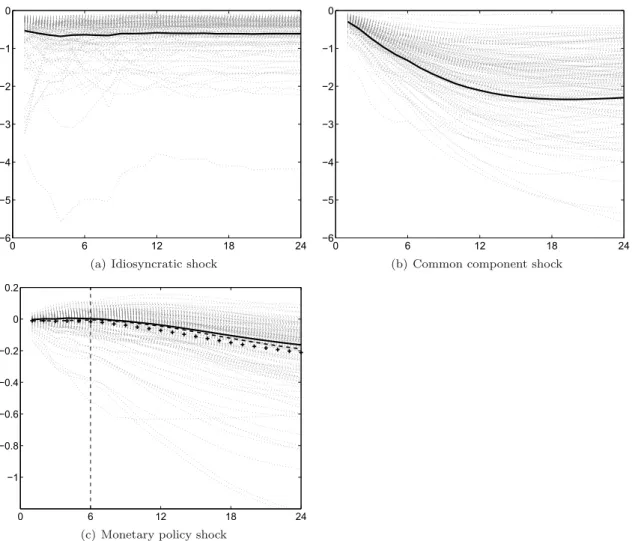
Panel (a) in Figure 2 shows the responses of each of the 151 CPI index items to an idiosyncratic shock of minus one standard deviation (dashed lines). The responses are calculated based on autoregressive processes fitted on the idiosyncratic component (cf. footnote 6). The solid line represents the weighted average response, where the weight of each index item in the CPI was averaged over the sample period. The figure indicates that the majority of price series responds very quickly to shocks in the idiosyncratic components. Most of the shocks are incorporated within one period. This pattern suggests that idiosyncratic shocks are only weakly autocorrelated. Since these shocks do not appear to have a persistent effect on disaggregate prices, the persistence in aggregate inflation rates is unlikely to be driven by idiosyncratic shocks. Panel (b) presents the responses of each CPI index item to a common component shock. Again, the responses stem from single autoregressive processes fitted on the common component. Therefore, the responses should be interpreted as an average response to a variety of underlying macroeconomic shocks. Prices react slowly to macroeconomic shocks. It takes about three years for most of the series to converge to their new level. We have additionally calculated the responses as weighted averages for various sectors such as goods and services or imported and domestic products. The main conclusions for all subaggregates are more or less the same: the response to an idiosyncratic shock is typically fast but it takes several years for a macroeconomic shock to feed fully into price changes.10
Prices may react very differently to various kinds of macroeconomic shocks such that the average responses displayed in Panel (b) may be misleading. Therefore, Panel (c) shows the responses of the disaggregate series to an identified monetary policy shock along with weighted and unweighted averages and the aggregate CPI. On average, we find a sluggish response of prices due to a monetary policy shock. Interestingly, there is substantial heterogeneity in the responses to a 25 basis point increase in the 3M Libor. Some series show a rapid decline, while others
Figure 2: Response of CPI index items to idiosyncratic, common component, and monetary policy shocks 0 6 12 18 24 −6 −5 −4 −3 −2 −1 0
(a) Idiosyncratic shock
0 6 12 18 24 −6 −5 −4 −3 −2 −1 0
(b) Common component shock
0 6 12 18 24 −1 −0.8 −0.6 −0.4 −0.2 0 0.2
(c) Monetary policy shock
Notes: Estimated impulse responses of CPI index items (in percent) to (a) an idiosyncratic shock of one standard deviation, (b) to a shock to the common component of one standard deviation and (c) to an identified monetary policy shock. (a) and (b) are based on autoregressive processes fitted on the idiosyncratic and common components and therefore represent average responses to a variety of idiosyncratic and macroeconomic shocks. The monetary policy shock is identified in the FAVAR framework. Thick solid lines represent weighted average responses. The monetary shock is a surprise increase of 25 basis points in the 3M Libor. The crosses in Panel (c) represent the unweighted average response, while the dashed line represents the response of the aggregate CPI to a monetary policy shock. The dashed vertical line shows the quarter at which the weighted average response turns negative.
display a hump-shaped response with prices first increasing after the monetary policy shock and decreasing afterwards.11
3.1.3 Sectoral heterogeneity
The sectoral responses to an identified monetary policy shock are informative in that they reveal that there is a lot of heterogeneity across sectors in the response. Moreover, we can also learn something from the sectoral heterogeneity itself, as the responsiveness to a monetary policy shock of a given sector can be matched with other characteristics from the sector, which makes it possible to evaluate whether the observed responses are consistent with various theories of price setting.
Recall from the descriptive analysis that the average persistence of the idiosyncratic component is close to zero (0.01), whereas the persistence of the common component is very high, at 0.84 (cf. Table 1). Together with the finding that the volatility of the idiosyncratic components of inflation are large on average and negatively correlated with the R2, measuring
the explanatory power of the common component for inflation, this evidence may support the rational inattention model presented in Mackowiak and Wiederholt (2009). Their theoretical model predicts that price-setting firms pay significantly more attention to idiosyncratic conditions than to macroeconomic conditions if the former are more volatile, implying that prices respond quickly to idiosyncratic shocks and slowly to macroeconomic shocks. Empirical support for this model has been found in Mackowiak et al. (2009) using a dynamic factor model based on sectoral CPI data estimated with Bayesian methods.
In what follows we shed light on this issue by explaining the cross-sectional variation of the monetary policy responses with features of their cross-sectional inflation dynamics. We therefore run regressions of the following form:
responsei,4 =α+β1sd(eit) +β2sd(λiCt) +β3ρ(eit) +β4ρ(λiCt) +εi . (4)
That is, we explain the accumulated response of CPI itemito a monetary policy shock after four
quarters in terms of the volatility and persistence of the idiosyncratic and common components. The specification differs from Boivin et al. (2009) in that it additionally includes the volatility and persistence of the common component. The descriptive statistics in Table 2 show that the volatility of the common component is correlated with the volatility of the idiosyncratic component,
11The impulse responses for several macroeconomic variables that might be of interest, although not directly
suggesting that the effect of idiosyncratic volatility might be overstated when excluding the volatility of the common component from the regressions.
Table 3: Cross-sectional variation of the accumulated monetary policy shock responses after 4 quarters
(1) (2) (3) (4) (5)
responsei,4 responsei,4 responsei,4 responsei,4 responsei,4
sd(eit) -0.079∗∗∗ -0.076∗∗∗ [0.009] [0.010] sd(λiCt) -0.067∗∗ -0.077∗∗ [0.029] [0.038] ρ(eit) 0.069∗∗∗ 0.006 [0.019] [0.010] ρ(λiCt) 0.204∗∗∗ -0.021 [0.065] [0.050] durationi 0.010∗∗∗ -0.007 [0.002] [0.005] sizei -0.261∗ -0.788∗∗∗ [0.141] [0.174] durationi×sizei 0.109∗∗∗ [0.032] Constant 0.056∗∗∗ -0.182∗∗∗ 0.075 -0.035 0.052∗ [0.006] [0.055] [0.048] [0.025] [0.029] Observations 151 151 151 124 124 R2 0.71 0.26 0.71 0.29 0.41
Notes: The duration is measured in quarters while the responses and standard deviations are measured in percent. The frequency and size of price changes are measured as fractions and rates of changes, respectively. The coefficients are estimated by OLS. Robust standard errors are given in brackets. *p <0.10, **p <0.05, ***p <0.01
The results are reported in Table 3. Column (1) suggests that the response to a monetary policy shock increases with the volatility of the idiosyncratic and common components.12 This actually
challenges the assumptions underlying the model proposed by Mackowiak and Wiederholt (2009), that firms, that face large idiosyncratic shocks, pay less attention to macroeconomic shocks. Their model would imply that larger idiosyncratic shocks would mitigate the response to a monetary policy shock after controlling for the volatility of macroeconomic shocks (cf. p. 98 Mackowiak et al., 2009). Our findings suggest that, even if we include the volatility of macroeconomic shocks in the regression, the sectors that are faced with larger idiosyncratic shocks incorporate the monetary
12As the dependent variable is the accumulated response to a tightening of monetary policy, the negative
coefficients imply that CPI items withmorevolatile idiosyncratic and common components show astronger decline
policy shock to a larger extent.13 This finding rather supports some of the menu-cost models, where
firms follow Ss-pricing rules, and idiosyncratic shocks rather than macroeconomic shocks trigger price adjustments. Such a model implies that a firm incorporates macroeconomic shocks once the idiosyncratic shock is large enough to push a firm’s price above the adjustment threshold.14 This
suggests that the source of price stickiness stems from menu costs rather than rational inattention. This contrasts the findings of Mackowiak et al. (2009) that sectors with more volatile idiosyncratic shocks imply a lower speed of response to macroeconomic shocks. While Mackowiak et al. (2009) restrict the analysis to price data only, we identify the common component using a large data set covering many aspects of the economy. To show the impact of restricting the data set to price data, we replicated the Mackowiak et al. (2009) model with monthly CPI data for Switzerland. It turns out that in this case the standard deviation of the common component is strongly negatively correlated (-0.91) with the standard deviation of the idiosyncratic component. This result would indeed suggest that firms react less to macroeconomic shocks in those sectors with volatile idiosyncratic shocks and it would favour the rational inattention model. Interestingly, we find the same correlation when we use our approach to identify the common components but limit the data set to price data. The negative correlation therefore rests on the fact that the common component is derived from the cross section of price data rather than from a broader data set with other macroeconomic variables. We prefer our approach because the identification of the common component is based on more information in a broader data set.
However, not only the volatility of the idiosyncratic and common components may affect the response to a monetary policy shock but also their persistence. Column (2) reports the estimated coefficients from regressing the accumulated responses on persistence. The persistence of both the common and the idiosyncratic shock mitigate the response to a monetary policy shock. In addition, we run a regression with all variables included. The coefficients are reported in Column (3). The volatility of common and idiosyncratic shocks are associated with a stronger response to a monetary policy shock, which corroborates the finding we have outlined earlier in the paper. The magnitude of the effect of the volatility is remarkably similar and the persistence measures are no longer significant when controlling for the volatility of common and idiosyncratic shocks. This suggests that the persistence of shocks is not responsible for cross-sectional differences in the reaction to monetary policy shocks. Also, theR2does not improve when including the persistence 13We replicated this result for the US with the data used inBoivin et al.(2009), which were kindly provided by
Marc Giannoni. After we excluded one outlier with implausibly high volatility of idiosyncratic shocks, which are driven by a structural break in the outlying series, the result holds for the response of sectoral prices up to six months after the identified monetary policy shock.
measures in the model with the volatility measures, and the explanatory power of the persistence measures alone is about three times smaller than the explanatory power of the volatility measures, which explain more than 70% of the differences in responsiveness to a monetary policy shock across sectors.
In addition, we test whether the cross-sectional differences in the responsiveness to a monetary policy shock can be associated with different degrees of price stickiness and the heterogeneity in price-setting behaviour. Boivin et al. (2009) examine the cross-sectional dispersion of price responses to a monetary policy shock focusing on the volatility and persistence of the idiosyncratic component, and measures of the degree of competition within each sector. They find that firms in industries with persistent and volatile idiosyncratic shocks react faster to monetary policy shocks. Furthermore, prices adjust more sluggishly in industries with a lower degree of competition. Our paper shows an interesting additional test to evaluate the different assumptions underlying the theoretical models since idiosyncratic shocks are on average more volatile than common component shocks (cf. Table 1). Therefore, rational inattention would predict that sectors with many price adjustments will tend to react slowly to macroeconomic shocks as these adjustments are likely to be associated with idiosyncratic shocks. By contrast, Carvalho (2006) shows that in a multi-sector Calvo model, heterogeneity in the frequency of price adjustments implies differences across sectors in the speed of adjustment to shocks, which leads to larger and more persistent real effects of monetary policy shocks. In this model, sectors with more price adjustments tend to react faster to macroeconomic shocks, but sectors with lower price adjustment frequencies have disproportionate effects on aggregate inflation persistence, because the sectors with more price adjustments take their slow adjustment into account when re-setting their prices. Thus, we examine whether the degree of price stickiness in a sector explains its degree of responsiveness to the monetary policy shock. Furthermore, we control for the average size of price adjustment within a sector, as the response of a given sector is also influenced by the average size of adjustment, and not just its frequency. To do so, we match the responses with statistics from CPI micro data15 and estimate
responsei,4 =α+β1durationi+β2sizei+β3durationi×sizei+εi (5)
15We essentially use the frequency and size statistics at the index item level fromKaufmann(2009) calculated
between 1993 and 2005. In some cases we have aggregated the statistics to a higher level, consistent with the CPI index items used in the FAVAR. Since we do not have micro data on all components (most importantly rents) the number of observations is smaller than in the previous regressions. Nevertheless, the Swiss data has the advantage that the statistics on the duration and size of price adjustments come from the same source as the CPI index items used in the FAVAR. This is not the case for US data.
wheredurationi = log(0.5)/log(1−fpci) gives the implied median duration of price spells for index
itemi, as a measure of price stickiness in sectori, wherefpcidenotes the average fraction of prices
that change in a given quarter. Meanwhile,sizei gives the corresponding absolute average size of
price adjustments in sector i. We find that a higher degree of price stickiness in a sector leads
to a smaller response to a monetary policy shock (Column 4). This is in line the assumptions underlying the model of Carvalho (2006) but not with the rational inattention model. Furthermore, the sectors that display a larger average absolute size of price adjustments are more responsive. This is in line with the findings from Columns (1) and (3) that the sectors that face larger shocks respond stronger to monetary policy shocks.
An unanswered question in the price-setting literature is whether menu costs are indeed a source of price rigidity and the resulting monetary non-neutrality. If that was the case, sectors with larger menu costs should adjust prices less frequently, but if they adjust, then they adjust by a large amount. Then we would expect the interaction term between the duration and absolute size of price adjustments to be positive, which would imply that the sectors with large menu costs are less responsive to a monetary policy shock and, on the aggregate, delay the overall response of the CPI. This is indeed the finding reported in Column (5). Sectors in which prices are adjusted infrequently, but by a large amount, are those that display a lower responsiveness to monetary policy shocks. With the inclusion of the interaction term, the duration variable is no longer significant. This suggests that indeed differences in menu costs may at least partially explain differences in monetary policy responsiveness. This finding is in line with the state-dependent pricing models that assume a distribution of menu costs across sectors to be responsible for monetary non-neutrality (cf. e.g. Dotsey et al., 1999; Nakamura and Steinsson, 2010).16
3.2
Monetary policy transmission
The FAVAR allows us to analyse the monetary policy transmission process in more detail. In particular, we analyse the speed of response in various sectors and the existence of a price puzzle.
16The regression results are consistent for various horizons of the responses. For longer horizons, the effects are
even more pronounced. We have added the responses for 8 quarters as a robustness check in the Appendix in Table9. In addition, we have repeated the regressions including the size and duration of price changes with the price responses to a common component shock. The results are remarkably similar, so that the conclusions apply to other macroeconomic shocks as well (cf. Table10in the Appendix).
3.2.1 The lag of monetary policy transmission
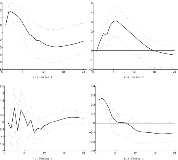
Let us first look at the responses of the factors (cf. Figure 3). 90% confidence intervals are given as dotted lines. They are derived via the bias-corrected bootstrap algorithm proposed by Kilian (1998). In line with much of the literature we ignore the fact that the factors are estimated and therefore subject to uncertainty. Note that we still obtain correct confidence intervals if the number of time series inXtis large relative to the number of time periods (cf. Bai and Ng, 2004).
Figure 3: Responses of the factors to an identified monetary policy shock
0 6 12 18 24 −6 −5 −4 −3 −2 −1 0 1 2 3 (a) Factor 1 0 6 12 18 24 −2 −1 0 1 2 3 4 5 (b) Factor 2 0 6 12 18 24 −2 −1.5 −1 −0.5 0 0.5 1 1.5 2 2.5 (c) Factor 3 0 6 12 18 24 −0.3 −0.2 −0.1 0 0.1 0.2 0.3 0.4 (d) Factor 4
Notes: Responses to an identified monetary policy shock along with 90% confidence intervals. The monetary shock is a surprise increase of 25 basis points in the 3M Libor. Factor 1 is the general prices factor, Factor 2 the (inverse) real activity factor and Factor 3 the factor of (foreign) goods prices with sales. Factor 4 shows the 3M Libor.
Figure 3 shows that the factor capturing price dynamics (Factor 1) exhibits a hump-shaped response. That is, inflation increases at first and then declines after roughly 7 quarters. As one
would expect, real activity declines after a contractionary monetary policy shock (shown in Panel b; recall that Factor 2 measures inverse real activity). It is interesting to see that Factor 3 does not react systematically to a monetary policy shock. As we have noted, it mainly captures the common dynamics of end-of-season sales prices. The interest rate (Factor 4) displays some inertia after the initial shock. It first raises slightly and then returns to zero after seven quarters.
Recall that Figure 2, Panel (c) gives the weighted average response of the CPI items along with the response of the aggregate CPI to a monetary policy shock. The weighted average of the responses (solid line) initially stays close to zero up to about 6 to 7 quarters and then starts to decline. This is consistent with the fact that price spells are long, slightly more than one year on average (cf. Kaufmann, 2009). A similar reaction is found for the aggregate CPI (dashed line). The unweighted average of the individual items displays a faster reaction (crosses).
3.2.2 The Swiss price puzzle: fact or artefact?
The literature has proposed various arguments for why econometricians tend to find a price puzzle, i.e. a rise in the aggregate price level in response to a contractionary innovation in monetary policy (for an overview cf. Walsh, 2003, Chapter 1). One is that the price puzzle is a “fact” and that prices do indeed rise after a monetary policy tightening. The theoretical argument here is that a cost channel of monetary policy exists. We discuss this first explanation in more detail in section 3.2.3 and now focus on the second explanation, which is that not enough information is included in usual three-variable VARs, and therefore the price puzzle is only an “artefact”.
Sims (1992) and many other studies found that including a commodity price index in the VAR reduces the price puzzle considerably (cf. also Eichenbaum, 1992). Also, Leeper and Zha (2001) stress that including money in the analysis removes the price puzzle (cf. Assenmacher-Wesche, 2008, for Switzerland). Giordani (2004) argues that typical VAR studies include GDP growth instead of an output gap measure. He shows that the omission of an output gap spuriously leads to a price puzzle in a class of commonly used models. Once an output gap measure is accounted for, the price puzzle disappears without including a commodity price index.
The FAVAR approach encompasses these arguments. The large data set reflects a larger share of the information available to a central bank than a typical three-variable VAR (with GDP, inflation and a short-term interest rate). Indeed, Bernanke et al. (2005) and Boivin et al. (2009) show for the US that the price puzzle found in standard VARs by and large disappears when augmenting a VAR by one or more factors.
If the information contained in the common factors was the sole reason why the price puzzle disappears we would expect that this also holds when we augment a standard three-variables VAR with our factors. The FAVAR model nests this VAR and therefore we can assess whether the additional information reduces the price puzzle (cf. Bernanke et al., 2005). We can illustrate the impact of more accurate information contained in the factors by using the factors from the FAVAR along with GDP, CPI inflation and the 3M Libor in a VAR where we identify the monetary policy shock by recursive ordering. Figure 4 illustrates how, by including one or two factors, the price puzzle by and large vanishes.17
Figure 4: Response to an identified monetary policy shock in a (FA)VAR
0 6 12 18 24 −0.1 0 0.1 0.2 0.3 (a) 3M Libor 0 6 12 18 24 −0.2 −0.1 0 (b) GDP 0 6 12 18 24 −0.1 0 0.1 (c) CPI
Notes: Estimated impulse responses (in percent) of the CPI and GDP to an identified monetary policy shock. The first VAR contains the CPI, GDP and the 3M Libor (solid line). The second and third VAR (dashed and dotted lines) contain additionally 1 and 2 factors according to the procedure byBernanke et al. (2005). The monetary shock is a surprise increase of 25 basis points in the 3M Libor.
17We have experimented with the inclusion of more factors and with total CPI excluding rents. The results do
3.2.3 Sectoral monetary policy responses
Figure 2, Panel (c), illustrates that, although prices react with a lag of 6 to 7 quarters on average, there is a large degree of heterogeneity across individual CPI index items. As noted earlier, heterogeneity in price stickiness and thus monetary policy responsiveness across sectors is important because it means that the real effects of monetary policy are more persistent (cf. Carvalho, 2006). The heterogeneity implies that sectors with lower price adjustment frequencies have disproportionate effects on aggregate price dynamics. Barsky et al. (2007) show that, even if most prices are flexible, a small durable goods sector with sticky prices may be sufficient to make aggregate output react to monetary policy as if most prices were sticky. Thus, the speed of the aggregate monetary policy response depends more crucially on the sectors with larger rigidities.
In this section, we show price responses for various sectors to an identified monetary policy shock. Figure 5 shows the response of the weighted average of all goods series to a monetary policy shock (Panel a). Interestingly, prices of goods decline immediately and significantly after such a shock. Meanwhile, the prices of services display a delayed response and are lowered only after 15 quarters (Panel b).
Figure 5: Response of goods and services prices to an identified monetary policy shock
0 6 12 18 24 −0.4 −0.2 0 0.2 (a) Goods 0 6 12 18 24 −0.4 −0.2 0 0.2 (b) Services
Notes: Estimated impulse responses (in percent) to an identified monetary policy shock along with 90% confidence intervals. The monetary shock is a surprise increase of 25 basis points in the 3M Libor. The impulse responses are aggregated from the individual CPI index items using the average CPI expenditure weight over the estimation period.
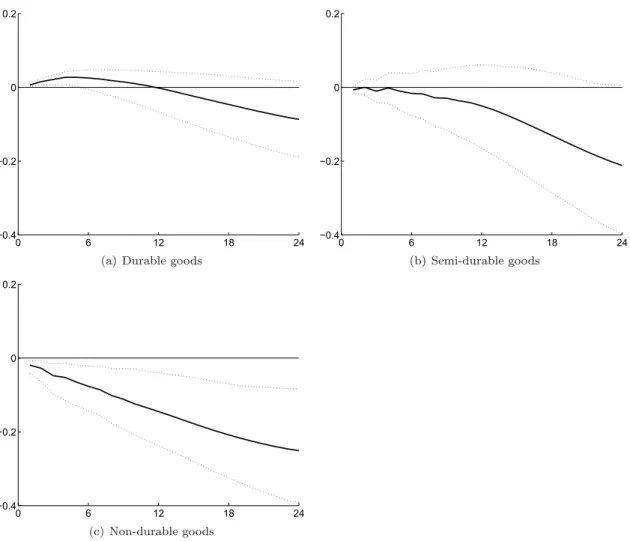
To obtain a more detailed picture of the response of goods prices, we have illustrated the responses of durable goods, semi-durable goods, and non-durable goods separately (cf. Figure 6). The reaction to unexpected monetary policy tightening shows some differences. Durable goods
prices start falling about 12 quarters after the shock. Meanwhile, semi-durable goods prices react with a lag of 4 quarters, and non-durable goods react instantaneously.
Figure 6: Response of durable, semi-durable and non-durable goods prices to an identified monetary policy shock
0 6 12 18 24
−0.4 −0.2 0 0.2
(a) Durable goods
0 6 12 18 24 −0.4 −0.2 0 0.2 (b) Semi-durable goods 0 6 12 18 24 −0.4 −0.2 0 0.2 (c) Non-durable goods
Notes: Estimated impulse responses (in percent) to an identified monetary policy shock along with 90% confidence intervals. The monetary shock is a surprise increase of 25 basis points in the 3M Libor. The impulse responses are aggregated from the individual CPI index items using the average CPI expenditure weight over the estimation period.
An explanation of why non-durable goods respond more quickly to monetary policy shocks than durable goods is that prices are more sticky in the durable goods sector. Based on the frequency of price changes presented by Kaufmann (2009), we can infer that prices of durable goods are stickier than prices of non-durable goods. The average duration of price spells for durable goods amounts to 4.2 quarters, while for non-durable goods it is 3.1 quarters. Semi-durable goods lie in
between.
unusual in that rents have a large weight in the Swiss CPI (on average 19.5%) and they are linked
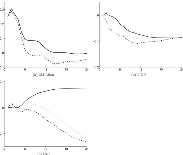
to mortgage rates by law (cf. Stalder, 2003). Owners of a rental apartment are usually allowed to change prices of rents under existing contracts when mortgage rates rise. Thus, higher interest rates may feed into higher rents and thus into the CPI. Panel (a) in Figure 7 shows the response of rents. Indeed, rents display a strong increase after monetary policy tightening. However, other services, as shown in Panel (b), still react with a significant delay of about 12 quarters to a monetary policy tightening.
Although we showed in Section 3.2.2 that the price puzzle can be resolved by the FAVAR approach, some sectors still exhibit a hump-shaped response to a monetary policy shock. This suggests that in these sectors the price puzzle is a “fact”. Theoretically, a hump-shaped price response may occur if higher interest rates translate into higher marginal costs of production. This is called the cost channel of monetary policy transmission.18 One explanation of a cost channel is
that firms hold working capital. To the extent that firms must pay the factors of production before receiving revenues from selling their products, they rely on borrowing from financial intermediaries, which makes their cost of production depend on the interest rates they have to pay for their loans. Similarly, if firms have to pre-finance inventories via financial intermediaries, higher interest rates can feed into higher prices as the real cost of inventories tend to increase on impact in response to monetary policy tightening.
Among the sectors which exhibit a significant hump-shaped response are durable goods. Arguably, inventory holdings are more important for durable goods than for non-durable goods and services. To the extent that firms have to finance their inventories in advance, monetary policy may temporarily lead to higher costs for inventory holdings and thus lead to higher prices. While there is a legal explanation for the hump-shaped response for rents, the impulse response function for other services is still puzzling. One explanation may be that the services sector depends more on external finance than the manufacturing sector, and thus the cost channel is more pronounced in the services sector. Some evidence in favour of this hypothesis is provided in de Serres et al. (2006), who show that most services industries rely more heavily on external finance than manufacturing industries.19 Another explanation may be that a high degree of real wage rigidity induces marginal
cost to adjust slowly. Together with the fact that the share of labour in total factor inputs is large for services, this is likely to amplify the cost channel of monetary policy because if the factors of production are pre-financed and unit labour costs are not flexible then prices of services are
18cf. e.g. Barth and Ramey (2002); Ravenna and Walsh (2006); Chowdhury et al. (2006); Rabanal (2007);
Figure 7: Response of rents, services prices excluding rents, and the CPI excluding rents to an identified monetary policy shock
0 6 12 18 24 −0.4 −0.2 0 0.2 (a) Rents 0 6 12 18 24 −0.4 −0.2 0 0.2
(b) Services excl. rents
0 6 12 18 24
−0.4 −0.2 0 0.2
(c) CPI excl. rents
Notes: Estimated impulse responses (in percent) to an identified monetary policy shock along with 90% confidence intervals. The monetary shock is a surprise increase of 25 basis points in the 3M Libor. The impulse responses are aggregated from the individual CPI index items using the average CPI expenditure weight over the estimation period.
likely to increase more strongly after monetary policy tightening compared to the case where unit labour costs are flexible.
We find support for these arguments in recent work on DSGE models which shows that the most important parameters for creating a hump-shaped response are those related to the degree of real wage rigidity. Rabanal (2007) shows in a calibrated new-Keynesian model that the presence of a cost channel is not sufficient to generate a positive response of inflation to monetary policy tightening. But when he introduces real wage stickiness, a hump-shaped response emerges. In an estimated version of this model for the US this feature disappears, however. By contrast, Henzel et al. (2009) show for the euro area that, although the cost channel does not produce a
hump-shaped response, it helps to explain a delayed inflation response. Our results are consistent with this body of the literature and suggest that, at the aggregate level, there is no price puzzle. But in sectors where inventory holdings or wage rigidities may play a larger role a hump-shaped response emerges leading to a more delayed response by the aggregate CPI.
4
Conclusions
In this paper, we analyse the response of disaggregate inflation rates to various macroeconomic shocks and idiosyncratic fluctuations, using a FAVAR approach. Additionally, we assess the impact of monetary policy on prices in various sectors. Looking at 151 disaggregated items from the Swiss CPI from 1978 Q1 to 2008 Q3, we find that disaggregate inflation rates react immediately to idiosyncratic shocks, whereas the reaction to macroeconomic disturbances and an identified monetary policy shock are sluggish and very heterogenous across sectors.
We analyse this heterogeneity in more detail and show that sectors with larger volatility of idiosyncratic shocks react more readily to monetary policy. This finding stands in contrast to the rational inattention model of price setting, which relies on the assumption that firms facing more idiosyncratic shocks react less strongly to aggregate shocks, because they pay less attention to them. We also find that sectors, which change prices infrequently, react less strongly but if they do change their prices, they adjust them by a large amount. This suggests that it is sectors with large menu costs that are responsible for the sluggish response rather than rational inattention.
Moreover, in line with findings for the US (Bernanke et al., 2005), the response of the aggregate CPI to a monetary policy shock no longer displays a price puzzle when applying the FAVAR methodology. The aggregate CPI is lowered 6 to 7 quarters after the monetary policy tightening. However, we find that durable goods and services prices show a very sluggish response to monetary policy tightening. This may be related to the cost channel of monetary policy. That gives an indication of the sectors that could be monitored more closely by monetary policy makers aiming to steer the aggregate inflation rate. The finding that rents exhibit a hump-shaped response can be explained by the fact that rents are linked to the mortgage rate in Switzerland.
References
Altissimo, F., B. Mojon, and P. Zaffaroni(2009): “Can Aggregation Explain the Persistence
of Inflation?” Journal of Monetary Economics, 56, 231–241.
Aoki, K. (2001): “Optimal monetary policy responses to relative-price changes,” Journal of
Monetary Economics, 48, 55–80.
Assenmacher-Wesche, K. (2008): “Modeling Monetary Transmission in Switzerland with a
Structural Cointegrated VAR Model,”Swiss Journal of Economics and Statistics (SJES), 144, 197–246.
Bai, J. and S. Ng(2002): “Determining the Number of Factors in Approximate Factor Models,”
Econometrica, 70, 191–221.
——— (2004): “Confidence Intervals for Diffusion Index Forecasts with a Large Number of Predictors,” Mimeo.
Barsky, R. B., C. L. House, and M. S. Kimball(2007): “Sticky-Price Models and Durable
Goods,”American Economic Review, 97, 984–998.
Barth, M. J. and V. A. Ramey (2002): “The Cost Channel of Monetary Transmission,” in
NBER Macroeconomics Annual 2001, Volume 16, National Bureau of Economic Research, Inc, NBER Chapters, 199–256.
Bernanke, B., J. Boivin, and P. S. Eliasz (2005): “Measuring the Effects of Monetary
Policy: A Factor-augmented Vector Autoregressive (FAVAR) Approach,”The Quarterly Journal of Economics, 120, 387–422.
Boivin, J., M. P. Giannoni, and I. Mihov (2009): “Sticky Prices and Monetary Policy:
Evidence from Disaggregated US Data,”American Economic Review, 99, 350–84.
Carvalho, C.(2006): “Heterogeneity in Price Setting and the Real Effects of Monetary Shocks,”
Frontiers of Macroeconomics, 2, 1–56.
Chowdhury, I., M. Hoffmann, and A. Schabert(2006): “Inflation Dynamics and the Cost
Channel of Monetary Transmission,”European Economic Review, 50, 995–1016.
Christiano, L. J., M. Eichenbaum, and C. L. Evans(1999): “Monetary policy shocks: What
de Serres, A., S. Kobayakawa, T. Slok, and L. Vartia(2006): “Regulation of Financial
Systems and Economic Growth in OECD Countries: An Empirical Analysis,” Economic Studies 46, 2006/2, OECD.
Dotsey, M., R. King, and A. L. Wolman(1999): “State-Dependent Pricing and the General
Equilibrium Dynamics of Money and Output,”Quarterly Journal of Economics, 114, 655–90. ——— (2006): “Inflation and Real Activity with Firm-Level Productivity Shocks: A Quantitative
Framework.” Mimeo.
Eichenbaum, M. (1992): “’Interpreting the Macroeconomic Time Series Facts: The Effects of
Monetary Policy’: by Christopher Sims,”European Economic Review, 36, 1001–1011.
Elmer, S. and T. Maag (2009): “The Persistence of Inflation in Switzerland: Evidence from
Disaggregate Data,” Working papers 09-235, KOF Swiss Economic Institute, ETH Zurich.
Gertler, M. and J. Leahy (2008): “A Phillips Curve with an S,s Foundation,” Journal of
Political Economy, 116, 533–572.
Giordani, P. (2004): “An Alternative Explanation of the Price Puzzle,” Journal of Monetary
Economics, 51, 1271–1296.
Golosov, M. and R. E. Lucas(2007): “Menu Costs and Phillips Curves,”Journal of Political
Economy, 115, 171–199.
Henzel, S., O. H¨ulsewig, E. Mayer, and T. Wollmersh¨auser(2009): “The Price Puzzle
Revisited: Can the Cost Channel Explain a Rise in Inflation after a Monetary Policy Shock?”
Journal of Macroeconomics, 31, 268 – 289.
Jordan, T. J., M. Peytrignet, and E. Rossi(2010): “Ten Years’ Experience with the Swiss
National Bank’s Monetary Policy Strategy,”Swiss Journal of Economics and Statistics (SJES), 146, 9–90.
Kaufmann, D. (2009): “Price-Setting Behaviour in Switzerland: Evidence from CPI Micro
Data,”Swiss Journal of Economics and Statistics (SJES), 145, 293–349.
Kilian, L. (1998): “Small-Sample Confidence Intervals For Impulse Response Functions,” The
Leeper, E. M. and T. Zha(2001): “Assessing Simple Policy Rules: A View From a Complete
Macroeconomic Model,”Federal Reserve Bank of St. Louis Review, 83–112.
Mackowiak, B., E. Moench, and M. Wiederholt (2009): “Sectoral Price Data and
Models of Price Setting,” Journal of Monetary Economics, 56, S78 – S99, supplement issue: December 12-13, 2008 Research Conference on ’Monetary Policy under Imperfect Information’ Sponsored by the Swiss National Bank (http://www.snb.ch) and Study Center Gerzensee (www.szgerzensee.ch).
Mackowiak, B. and M. Wiederholt (2009): “Optimal Sticky Prices under Rational
Inattention,”American Economic Review, 99, 769–803.
Midrigan, V. (2008): “Is Firm Pricing State or Time-Dependent? Evidence from US
Manufacturing,”Review of Economics and Statistics, forthcoming.
Mumtaz, H., P. Zabczyk, and C. Ellis(2009): “What Lies Beneath: What Can Disaggregated
Data Tell us About the Behaviour of Prices?” Working Paper 364, Bank of England.
Nakamura, E. and J. Steinsson (2010): “Monetary Non-Neutrality in a Multisector Menu
Cost Model,” The Quarterly Journal of Economics, 125, 961–1013.
Rabanal, P. (2007): “Does Inflation Increase after a Monetary Policy Tightening? Answers
Based on an Estimated DSGE Model,”Journal of Economic Dynamics and Control, 31, 906 – 937.
Ravenna, F. and C. E. Walsh (2006): “Optimal Monetary Policy with the Cost Channel,”
Journal of Monetary Economics, 53, 199–216.
Sims, C. A.(1992): “Interpreting the Macroeconomic Time Series Facts : The Effects of Monetary
Policy,” European Economic Review, 36, 975–1000.
Stalder, P. (2003): “The Decoupling of Rents from Mortgage Rates: Implications of the Rent
Law Reform for Monetary Policy,” SNB Quarterly Bulletin 3, Swiss National Bank.
Stock, J. H. and M. W. Watson (2002): “Macroeconomic Forecasting Using Diffusion
Indexes,”Journal of Business & Economic Statistics, 20, 147–62.
Tillmann, P. (2008): “Do Interest Rates Drive Inflation Dynamics? An Analysis of the
Cost Channel of Monetary Transmission,” Journal of Economic Dynamics and Control, 32, 2723–2744.
Appendices
A
Supplementary figures
Figure 8: Output gap versus inverse real activity factor
1975 1980 1985 1990 1995 2000 2005 2010 −5 −4 −3 −2 −1 0 1 2 3 4 5 1975 1980 1985 1990 1995 2000 2005 2010 −1 −0.8 −0.6 −0.4 −0.2 0 0.2 0.4 0.6 0.8 1
Notes: The figure gives an output gap measure (in percent) calculated by the Swiss National Bank according to a production function approach (dashed line). In addition, it gives the real activity factor (solid line, inverse right-hand scale).
Figure 9: Response of key macroeconomic variables to an identified monetary policy shock (monetary aggregates) 0 6 12 18 24 −0.6 −0.4 −0.2 0 0.2 0.4 0.6 0.8
(a) Monetary base
0 6 12 18 24 −0.8 −0.6 −0.4 −0.2 0 0.2 0.4 0.6 0.8 1 1.2 (b) M1 0 6 12 18 24 −1 −0.8 −0.6 −0.4 −0.2 0 0.2 0.4 (c) M2 0 6 12 18 24 −0.3 −0.25 −0.2 −0.15 −0.1 −0.05 0 0.05 0.1 0.15 0.2 (d) M3
Notes: Estimated impulse responses (in percent) to an identified monetary policy shock along with 90% confidence intervals. The monetary shock is a surprise increase of 25 basis points in the 3M Libor.
Figure 10: Response of key macroeconomic variables to an identified monetary policy shock (interest rates) 0 6 12 18 24 −0.15 −0.1 −0.05 0 0.05 0.1 0.15 0.2
(a) Mortgage rate
0 6 12 18 24 −0.1 −0.05 0 0.05 0.1 0.15 0.2 0.25
(b) Government bonds (10y)
0 6 12 18 24 −0.3 −0.2 −0.1 0 0.1 0.2 0.3 0.4 (c) 3M Libor 0 6 12 18 24 −0.2 −0.15 −0.1 −0.05 0 0.05 0.1 0.15 (d) Spread
Notes: Estimated impulse responses (in percent) to an identified monetary policy shock along with 90% confidence intervals. The monetary shock is a surprise increase of 25 basis points in the 3M Libor.
Figure 11: Response of key macroeconomic variables to an identified monetary policy shock (consumer prices) 0 6 12 18 24 −0.4 −0.35 −0.3 −0.25 −0.2 −0.15 −0.1 −0.05 0 0.05 0.1
(a) Consumer prices
0 6 12 18 24 −0.45 −0.4 −0.35 −0.3 −0.25 −0.2 −0.15 −0.1 −0.05 0 0.05
(b) Consumer prices: goods
0 6 12 18 24 −0.35 −0.3 −0.25 −0.2 −0.15 −0.1 −0.05 0 0.05 0.1 0.15
(c) Consumer prices: services
0 6 12 18 24 −0.4 −0.35 −0.3 −0.25 −0.2 −0.15 −0.1 −0.05 0 0.05
(d) Consumer prices excl. rents
0 6 12 18 24 −2.5 −2 −1.5 −1 −0.5 0 0.5 1 1.5 2 2.5
(e) Expected consumer prices
Notes: Estimated impulse responses (in percent) to an identified monetary policy shock along with 90% confidence intervals. The monetary shock is a surprise increase of 25 basis points in the 3M Libor.
Figure 12: Response of key macroeconomic variables to an identified monetary policy shock (prices and exchange rates prices)
0 6 12 18 24 −0.45 −0.4 −0.35 −0.3 −0.25 −0.2 −0.15 −0.1 −0.05 0 0.05
(a) Prices of total supply
0 6 12 18 24 −2.5 −2 −1.5 −1 −0.5 0 0.5 1 1.5 2 (b) Commodity prices 0 6 12 18 24 −4 −3 −2 −1 0 1 2 3 (c) Oil price 0 6 12 18 24 −2.5 −2 −1.5 −1 −0.5 0 0.5 1 1.5
(d) Expected wholesale prices
0 6 12 18 24 −1.5 −1 −0.5 0 0.5 1 (e) CHFUSD 0 6 12 18 24 −0.5 −0.4 −0.3 −0.2 −0.1 0 0.1 0.2 0.3 0.4 0.5 (f) CHFEUR
Notes: Estimated impulse responses (in percent) to an identified monetary policy shock along with 90% confidence intervals. The monetary shock is a surprise increase of 25 basis points in the 3M Libor.