DOI 10.1007/s10626-014-0195-5
Model approximation for batch flow shop scheduling
with fixed batch sizes
W. Samuel Weyerman·Anurag Rai·Sean Warnick
Received: 9 January 2012 / Accepted: 30 April 2014 / Published online: 7 June 2014 © Springer Science+Business Media New York 2014
Abstract Batch flow shops model systems that process a variety of job types using a fixed infrastructure. This model has applications in several areas including chemical manufac-turing, building construction, and assembly lines. Since the throughput of such systems depends, often strongly, on the sequence in which they produce various products, scheduling these systems becomes a problem with very practical consequences. Nevertheless, opti-mally scheduling these systems is NP-complete. This paper demonstrates that batch flow shops can be represented as a particular kind of heap model in the max-plus algebra. These models are shown to belong to a special class of linear systems that are globally stable over finite input sequences, indicating that information about past states is forgotten in finite time. This fact motivates a new solution method to the scheduling problem by optimally solving scheduling problems on finite-memory approximations of the original system. Error in solutions for these “t-step” approximations is bounded and monotonically improving with increasing model complexity, eventually becoming zero when the complexity of the approximation reaches the complexity of the original system.
Keywords Model approximation·Batch flow shop·Scheduling·Max-plus
W. S. Weyerman
Google, 1600 Amphitheatre Parkway Mountain View, CA, 94043, USA A. Rai
Laboratory for Information and Decision Systems, Massachusetts Institute of Technology, Cambridge, MA, 02139, USA
S. Warnick ()
Information and Decision Algorithms Laboratories, Department of Computer Science, Brigham Young University, Provo, UT, 84602, USA
1 Introduction
Production systems have a rich history and employ a variety of mathematical models to understand their dynamics. The batch flow shop model is a general model class that represents the production of multiple products, generally referred to a job types, using a fixed infrastructure, or set of resources or machines. The complexities of these systems make it difficult to characterize and analyze these models. Nevertheless, the batch flow shop model is useful for several applications, including flowshops, chemical processing plants, and various services. Some specific examples of these application areas are pharmaceutical production, propellant manufacturing, building construction, and assembly lines.
One of the key questions one would like to understand in a production system is how to optimally schedule factory resources when processing a suite of job types. This turns out to be a hard problem. Nevertheless, a variety of models and simplifications have been studied to gain insight about this problem, including exact methods attempting to solve large integer programs (Rich and Prokopakis1986; Kondili et al.1993) and the scheduling of a single machine (French1982; Parker1995; Pinedo2005). Many different objectives are specified in Pinedo (2005); these objectives introduce ideas such as minimum makespan, maximum throughput, minimum (weighted) tardiness, minimum lead time, and so on. In van Eekelen et al. (2006) and Boccadoro and Valigi (2003) an optimal 2-product cyclical schedule is determined for a single machine with setup costs. A natural extension to this problem is that of scheduling a job shop with multiple machines. The problem of scheduling several jobs on a set of machines with infinite queues is covered extensively in Pinedo (2005). Other models include a method of treating manufacturing systems as continuous systems in time and controlling them using linear programming is given in van Eekelen et al. (2005), and the so-called “hot ingot” problem, or continuous processing flowshop, which requires a scheduled job to move to the next machine in its route with no delay. The “hot ingot” problem is shown to be equivalent to a single machine with sequence dependent setup times in Reddi and Ramamoorthy (1972). When sequence dependent setup times are added to the flowshop, the sequencing problem is shown to be equivalent to a traveling salesman problem in Gupta (1986). Savkin (2003) considers scheduling a “flexible manufacturing” system, where multiple job types are processed on the same set of machines. Nevertheless, in this work, unbounded buffers are included between each machine, effectively decoupling the interprocessing dynamics.
A more complex environment, and the one we consider, is that with batching machines. Batching machines may process several jobs of a given type simultaneously, but each machine has a fixed batch capacity. Scheduling these systems breaks down into two main problems that need to be solved: lot sizing and scheduling. The lot sizing problem is to deter-mine how many jobs to process at a given time and is discussed in Deng et al. (2002), Dupont and Dhaenens-Flipo (2002) and Glass et al. (2001). The sequencing problem is to determine the order in which to process the jobs to optimize some objective. For our work, we assume that the lot sizing problem has been solved, meaning the capacities of the machines is deter-mined a priori. Since lot sizes are fixed, solving the sequencing problem is all that is needed to solve the scheduling problem, and we will therefore use these terms interchangeably. As with the job shop, there has been considerable effort studying situations where one or two batching machines are present, such as Cheng et al. (2004), Hochbaum and Landy (1997), Lin and Cheng (2001) and Dobson and Nambimadom (2001). In Cheng et al. (2004) a vari-ation of the single machine batch scheduling problem is shown to be NP-Hard. A branch and bound algorithm for lot-sizing and scheduling of a single batch machine is given in Jordan and Drexl (1998). A two-machine factory is considered in Ahmadi et al. (1992)
where one or both machines is a batch machine. These authors consider the sequencing of jobs in the system using full batches and permutation schedules. However, they are limited to two machines and only one machine per workstation. They also simplify the problem by considering a batch machine that has a constant running time for any batch of jobs. Graphi-cal solutions to the general multipurpose batch plant are given in Sanmart´ı et al. (2002), Rich and Prokopakis (1986) and Kondili et al. (1993), but since these methods are exact, they are also computationally intractable for a complex manufacturing system. Two heuristic meth-ods of solution to the minimum makespan problem are given in Bl¨omer and G¨unther (1998), the better of the two reduces decision variables in the MILP by a linear factor. Although this does allow for the solution of more complex problems, it is still difficult to compute the makespan for a manufacturing system containing a workstation with a much larger capac-ity or longer processing time than another workstation. Other approaches to scheduling include solving a stochastic integer programming problem, Sand and Engell (2004), and a hybrid constraint logic programming (CLP) and mixed integer linear programming (MILP) approach, Roe et al. (2005). Bemporad (2003) and Corona et al. (2005) consider optimiza-tion in the face of quantizaoptimiza-tion and partioptimiza-tion the state space offline to facilitate fast decision making.
Much of the analysis and modeling of job shops and manufacturing systems is done using discrete event systems. Multipurpose batch manufacturing systems are modeled as Petri nets in Riera et al. (2005), Yajima et al. (2004), L´opez-Mellado et al. (2005). An optimization procedure for Petri nets is also given in Riera et al. (2005), however, it is exact and thus not tractable for complex systems, so they offer a tree pruning heuristic to reduce the search time. A method for representing Petri nets as heaps of pieces in the max-plus algebra is given in Gaubert and Mairesse (1999), and much of our work is built on this foundation. Certain discrete event processes are shown to be linear in the max-plus algebra in Cohen et al. (1985) and Baccelli et al. (1992). They note that this is useful for performance evaluation in manufacturing. Other approaches to scheduling using max-plus models include Yurdakul and Odrey (2004), Bouquard et al. (2006a), Bouquard et al. (2006b), and Van den Boom and De Schutter (2006).
In this work we show that a batch flow shop can be modeled as an input quantized system in the max-plus algebra. This development is done by modeling the system as a heap of “non-rigid” pieces, in stark contrast to previous work using heaps of “rigid blocks”. Doing this, we show that the batch flow shop models are a subset of a larger class of systems in the max-plus algebra, a class that can be shown to be globally stable over finite-length inputs. This stability property causes these systems to forget initial condition information in a finite number of steps and motivates our approximation method. Our approach is to optimally solve the sequencing problem for asimplifiedmodel of the batch flow shop (Beck et al.1996; Dullerud and Paganini2000). The organization of this paper is as follows. We first present the max-plus algebra. This allows us to introduce the batch flow shop model and represent it as a max-plus dynamical system. We show that batch flow shops are a subset of a larger class of systems in the max-plus algebra that exhibit a particular structure. We then show that any system in this class exhibits a form of stability. We finally present our method of model approximation over this class of systems and show that this method has bounded error.
2 Max-plus algebra preliminaries
This work draws from the standardheaps of piecesorheap modelthat is described using the max-plus algebra, see for example Gaubert and Mairesse (1999), Heidergott et al. (2006).
These models describe situations like the popular Tetris game, where pieces of vari-ous shapes and orientations pile up vertically. This stacking mechanism is conveniently described as a linear system defined over the max-plus (or sometimes called tropical) semiring, described briefly below, along with definitions of system stability and various performance measures.
2.1 Background and notation
Definition 1 The (max, +) semiring,Rmax, is the setR∪ {−∞,+∞}, equipped with the operations
1. ⊕, wherea⊕b:=max(a, b), 2. ⊗, wherea⊗b:=a+b,
whereRis the set of real numbers. Note that often the symbolRmaxis used to indicate the complete (max, +) semiring, defined overR∪ {−∞,+∞}, but in this work, where there should be no confusion about the meaning, we remove the overline to simplify notation. Also, note that this semiring is idempotent, sincex⊕x = x for allx ∈ Rmax; the zero element is negative infinity, denoted; and the unit element is zero, denotede.Moreover, in this work, we will further consider the multiplicative inverse operation,, whereab:= a−b for all{a, b} ∈ Rmax, makingRmax a semifield. Throughout this paper we will use the convention = , suggesting that for anyy ∈Rmax, the indeterminate form
y⊕()=y.
Matrix arithmetic is also defined over the (max,+) semiring. For matrices,A, B∈Rnmax×l,
C∈Rlmax×mwe define the operations:
[A⊕B]ij := aij⊕bij [B⊗C]ik := l j=1 bij⊗cj k .
The zero vector,, and the unit vector,e, are given by
:= ⎡ ⎢ ⎣ .. . ⎤ ⎥ ⎦, e := ⎡ ⎢ ⎣ e .. . e ⎤ ⎥ ⎦,
whereeandare as defined above. The identity matrix is
Imax:= ⎡ ⎢ ⎢ ⎢ ⎣ e . . . e .. . . .. ... . . . e ⎤ ⎥ ⎥ ⎥ ⎦.
Spectral theory is well developed over the max-plus semiring. The following definition will be useful in the subsequent development in later sections.
Definition 2 (Heidergott et al.2006) LetA ∈Rnmax×nbe a square matrix. Ifμ∈Rmaxis a scalar andv∈Rnmaxis a vector that contains at least one finite element such that
A⊗v=μ⊗v,
We can now define a linear state-space system in the max-plus algebra. Forx(k)∈Rn
max,
k∈N, whereNdenotes the non-negative integers, andA∈Rnmax×n, the sequence generated by the recursion,
x(k+1)=A⊗x(k), (1)
is well-defined and characterized by
x(k)=A⊗kx0,
wherex(0)=x0∈Rnmaxis the initial condition, andA⊗kdenotes the matrixAraised to the
kthpower, in the max-plus sense of matrix multiplication. Similarly, if the system is time-varying, such as
x(k+1)=A(k)⊗x(k), (2)
the solution is well-defined and characterized by
x(k)= k−1 i=0 A(i) x0,
wherex(0)=x0∈Rnmaxis the initial condition. 2.2 Rigid-block heap models
These max-plus linear systems, such as that in Eq.2), are the basis for a standardheap model
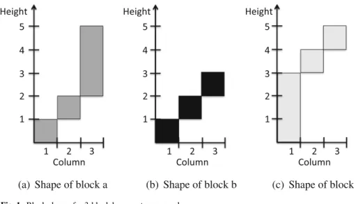
(Gaubert and Mairesse1999) that describes the surface of a pile of predefined, rigid blocks, or pieces. Like the game Tetris, imagine a stack of blocks that have piled up vertically, as in Fig.2. Unlike the Tetris game, however, these blocks do not rotate or move horizontally; each block is characterized by a well-defined shape over specific columns. We associate, then, each block with a particular matrix,A(i)∈Rnmax×n,i =1, . . . , m, wheremis the total number of distinct block types, and the vectorx(k)∈Rnmaxdescribes the height of the stack in each of thencolumns after thekthblock is added to the pile. The max-plus linear system (2) computes the changing surface vector,xas each new block is added (Fig1).
(a) Shape of block a (b) Shape of block b (c) Shape of block c
For example, consider the 3-block system characterized in Table1. In this system, there are three distinct shapes of blocks, labeleda,bandc, constructed over three columns. Two vectors inR3max characterize each block by defining its upper contour, u(p), and lower contour,l(p), and these contour vectors are then used to construct a matrix,A(p), associated with each block type,p∈ {a, b, c}, as follows:
[A(p)]ij = ⎧ ⎨ ⎩ ui(p)−lj(p)ifi, j∈R(p) e ifi=j,i /∈R(p) otherwise (3)
whereR(p)is the set of columns occupied by block typep.
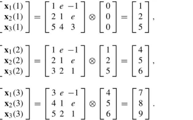
Starting from an “empty floor,”x(0) = 0 0 0T, the changing surface of the stack of blocks, or heap, driven by the input sequence a,b,c is then captured by the dynamics described in Eq.2as follows:
⎡ ⎣xx12((11)) x3(1) ⎤ ⎦= ⎡ ⎣12 1e −e1 5 4 3 ⎤ ⎦⊗ ⎡ ⎣00 0 ⎤ ⎦= ⎡ ⎣12 5 ⎤ ⎦, ⎡ ⎣xx12((22)) x3(2) ⎤ ⎦= ⎡ ⎣12 1e −e1 3 2 1 ⎤ ⎦⊗ ⎡ ⎣12 5 ⎤ ⎦= ⎡ ⎣45 6 ⎤ ⎦, ⎡ ⎣xx12((33)) x3(3) ⎤ ⎦= ⎡ ⎣34 1e −e1 5 2 1 ⎤ ⎦⊗ ⎡ ⎣45 6 ⎤ ⎦= ⎡ ⎣78 9 ⎤ ⎦.
This sequence of blocks a,b,c, results in the surface vectorx(3)=7 8 9T, as illustrated in Fig.2.
2.3 Stability and performance measures
Throughout this paper we will be interested in the behavior of max-plus linear systems, such as that in Eq.2, for largek. The following definitions will help clarify the resulting analysis (Table2).
Table 1 Mathematical modeling of a 3-block system
Block Upper contour Lower contour Matrix representation
a u(a)= ⎡ ⎢ ⎣ 1 2 5 ⎤ ⎥ ⎦ l(a)= ⎡ ⎢ ⎣ e 1 2 ⎤ ⎥ ⎦ A(a)= ⎡ ⎢ ⎣ 1 e −1 2 1 e 5 4 3 ⎤ ⎥ ⎦ b u(b)= ⎡ ⎢ ⎣ 1 2 3 ⎤ ⎥ ⎦ l(b)= ⎡ ⎢ ⎣ e 1 2 ⎤ ⎥ ⎦ A(b)= ⎡ ⎢ ⎣ 1 e −1 2 1 e 3 2 1 ⎤ ⎥ ⎦ c u(c)= ⎡ ⎢ ⎣ 3 4 5 ⎤ ⎥ ⎦ l(c)= ⎡ ⎢ ⎣ e 3 4 ⎤ ⎥ ⎦ A(c)= ⎡ ⎢ ⎣ 3 e −1 4 1 e 5 2 1 ⎤ ⎥ ⎦
Fig. 2 Heap resulting from stacking blocksa,b, andc
Definition 3 The system given by Eq.1and characterized by the matrixA∈Rnmax×nis said to beglobally stableif, for any initial conditionx(0):
∃N∈Nand uniquev1, ..., vn∈Rsuch that k≥N =⇒ xi(k)x1(k)=vi, whereNis understood to be the set of natural numbers.
Global stability implies that, after a finite number of steps, the relative distance among the elements ofx(k)remains fixed ask→ ∞. This suggests a notion of convergence in a projective space, formed as the quotient space ofRnmaxby a particular equivalence relation (see Section 1.4 in Heidergott et al. (2006) for details). In particular, while the values of the elements of the state vector of a globally stable system may grow without bound, the relative differences among elements ofxremain constant after some initial transient period. Moreover, this limiting behavior ofxis unique, independent of the initial condition.
In addition to the limiting behavior characterized by global stability, we will also be interested in various measures characterizing the quality of our approximations. In particu-lar, we will abuse notation and consider the following functions that are not norms, but are reminiscent of these measures and will be useful in the sequel.
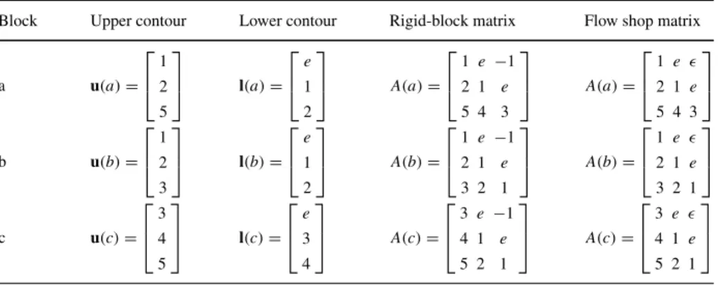
Table 2 Comparing rigid-block heap matrices with flow shop heap matrices
Block Upper contour Lower contour Rigid-block matrix Flow shop matrix
a u(a)= ⎡ ⎢ ⎣ 1 2 5 ⎤ ⎥ ⎦ l(a)= ⎡ ⎢ ⎣ e 1 2 ⎤ ⎥ ⎦ A(a)= ⎡ ⎢ ⎣ 1 e −1 2 1 e 5 4 3 ⎤ ⎥ ⎦ A(a)= ⎡ ⎢ ⎣ 1 e 2 1 e 5 4 3 ⎤ ⎥ ⎦ b u(b)= ⎡ ⎢ ⎣ 1 2 3 ⎤ ⎥ ⎦ l(b)= ⎡ ⎢ ⎣ e 1 2 ⎤ ⎥ ⎦ A(b)= ⎡ ⎢ ⎣ 1 e −1 2 1 e 3 2 1 ⎤ ⎥ ⎦ A(b)= ⎡ ⎢ ⎣ 1 e 2 1 e 3 2 1 ⎤ ⎥ ⎦ c u(c)= ⎡ ⎢ ⎣ 3 4 5 ⎤ ⎥ ⎦ l(c)= ⎡ ⎢ ⎣ e 3 4 ⎤ ⎥ ⎦ A(c)= ⎡ ⎢ ⎣ 3 e −1 4 1 e 5 2 1 ⎤ ⎥ ⎦ A(c)= ⎡ ⎢ ⎣ 3 e 4 1 e 5 2 1 ⎤ ⎥ ⎦
Definition 4 The 1-measure of a max-plus vector,b∈Rn maxis ||b||1max = n i=1 bi=eT ⊗b.
Note that this function returns the maximum element of a vector. Moreover, this function induces a similar function on a matrix.
Definition 5 The max-plus 1-induced measure of a matrixA∈Rnmax×mis
||A||1max = max
x∈Rm×1 max,x=
(||A⊗x||1max ||x||1max).
Lemma 1 Given a matrixA∈Rnmax×m, the max-plus 1-induced measure ofAis equivalent to its largest element:
||A||1max =max
ij aij.
Proof LetA∈Rmaxn×mbe given. Without loss of generality, we will say that||x||1max =e. Note that||A⊗x||1max = eT ⊗A⊗x. The vector vT =: eT ⊗A is the vector con-taining the max element of each column ofA. Therefore, we want to maximizevT ⊗x. Because||x||1max =e, the largest element inxise. To maximizevT⊗x, we want to make each element ofxas large as possible; this means we setx = ewhich givesvT ⊗x =
maxijaij.
By this theorem, we see that the max-plus 1-induced measure of a matrix is very simple to compute. We are also interested in a similar quantity, minxA⊗x1max x1max. This quantity is also simple to compute.
Lemma 2 Given a matrixA∈Rnmax×m,
min x∈Rm×1 max,x= ||A⊗x||1max ||x||1max =min i eT ⊗A i.
Proof LetA ∈Rmaxn×mbe given. Without loss of generality, let||x||1max = eand consider
vT ⊗xwithvT =:eT ⊗A. Now we want to minimizevT ⊗x, so we want each element ofxas small as possible. However, having||x||1max =erequires at least one element ofx equal toe. Thus, we need only consider eachxwherexi=e, andxj =forj=i. So
min x vT ⊗x = min i (vi) = min i eT ⊗A i.
3 Model for a batch flow shop
Consider a batch flow shop model given by nworkstations that operates on m distinct job types. As a flow shop, each job type follows the same route through the system and workstations are ordered accordingly. We restrict our attention to the situation where there
is no intermediate storage between the machines (however the machines themselves can store the load whenever necessary) and each workstation is composed of a single machine.
We focus on the sequencing problem by assuming that the lot sizing problem has previ-ously been solved. This defines a fixed capacity for each job type,j, on each workstationi,
cij. Likewise, each job type has a fixed processing time on each workstation,τij, yielding
the recipe(c,τ)(j )for every job typej ∈J = {1, . . . , m}.
Fixed routes, no intermediate storage, and fixed capacities restrict admissible sched-ules for the system to be permutation schedsched-ules. That is, each workstation must follow the same sequence of job types. Furthermore, by imposing a non-idling policy, every sequence uniquely specifies an admissible schedule for the system.
The fact that the capacity of the first workstation is fixed for each job type implies that commanding a particular job type requires at least the number of jobs of this type to fill the capacity of the first workstation. Moreover, since other workstations may have different capacities for the same job type, more than one batch may be required of the first work-station. For example, if capacity of the second workstation is twice that of the first, then commanding this job type will require at least two batches from the first workstation. The least common multiple of the workstation capacities for a given job typej, called the load,
L(j ), is the minimum number of jobs of this type that must be commanded to satisfy the workstation capacities and admissibility requirements of the system. From this we see that workstationimust processB(i)=L(j )/cijbatches of job typejto complete a load.
These requirements imply that the scheduling problem consists of choosing a sequence of loads of various job types to meet a specified quotaq∈Nm, whereNis the set of natural
numbers. LetQ = mi=1qi. Only quotas that are integer multiples of loads for each job type make sense. This sequence of loads,uk∈J,k=0, . . . , Q, is the input to the system, which we will represent as evolving with load-events,k, rather than in real time.
The state of the system,x(k) ∈ Rn, represents the time at which each workstation is available for processing the kth load. The system output, y(k), represents the transition time from statex(k)to x(k+1), which is the time it takes to finish the (k+1)th load
after finishing thekthload. We note that the dynamics of this system are not linear in the convential algebra. As a result, we will characterize this system as a discrete-time dynamical system with linear dynamics (albeit a nonlinear output function) over the max-plus semiring as a modified heap model.
3.1 Max-plus representation
The heap model discussed previously makes a nearly ideal model for the flow shop described above. In the heap model, blocks are defined by their shape, characterized by height over a fixed set of columns. In the flow shop, each load is also defined by a shape, characterized by the amount of time it requires from each workstation, over a fixed set of workstations. We see, then, that the state of the system,x(k)∈Rnmax, representing the time when each of thenworkstations is available for processing thekthload, evolves as Eq.2,
where each job typej ∈ J = {1, . . . , m}is associated with a matrixA(j )∈ Rnmax×n. An empty flow shop begins fromx(0) =eand processesQloads, defining a sequencex(k),
k=0, ..., Q−1, to meet its quota.
There are some important differences, however, between the rigid-block heap model discussed previously, and a heap model capable of describing the dynamics of the flow shop described above. First, in the flow shop considered here, a non-idling policy is enforced. This ensures that every sequence of loads generates a unique admissible schedule, thereby reducing the scheduling problem to a sequencing problem. It also implies, however, that if a
machine is available and the next load is ready, then it should start processing the next load, which (along with the no-intermediate-storage policy) can warp the “shape” associated with the next load.
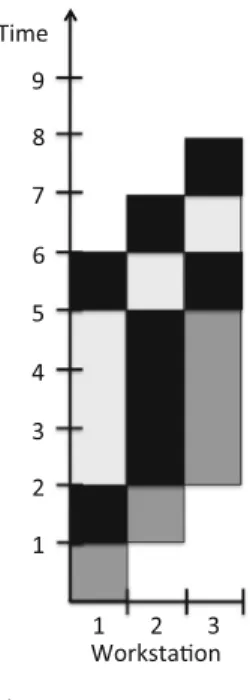
For example, consider Fig.2. If we associate loads with blocks, columns with worksta-tions, and the height of a block with the time that load requires from each workstation, then we see immediately that a non-idling policy would warp the shape of block, or load,b. This is because workstation 1 becomes available after processing its first load (of job-typea) at time 1, so it should then immediately begin processing loadb. Workstation 1 will finish processing loadbat time 2, the exact same time when workstation 2 finishes processing loada. As a result, it will then unloadbinto workstation 2, which will immediately begin processing loadb. Workstation 2 will finish processing loadbat time 3. Nevertheless, the no-intermediate-storage policy indicates that Workstation 2 can not unloadbuntil time 5, when Workstation 3 completes its processing of loada, further warping the shape of loadb. Figure3illustrates how the flow shop dynamics considered here would process the three jobs from Table1. Notice that, unlike Fig. 2, here the blocks representing loads are not rigid. For example, in Fig.3b we note that, even in the same sequence, the shape of loadb
can be different, depending on the state of the system when it is processed. This important difference between the flow shop model and the rigid-block heap model enables the flow
(a)Quota {a,b,c} completed two time units sooner than the rigid-block heap model shown in Figure 2.
(b) Processing an additional load of b highlights how the shape associated with load b (black piece) changes due to the non-idling and no-intermediate-storage policies of the flow shop, demanding a new heap model.
Fig. 3 Flow shop heap resulting from processing loadsa,b, andc(left) and another load ofb(right) from the heap example in Table1
shop to process a given quota faster than its rigid-block counterpart. For example, in Fig.3a, the same sequence,a,b, andc, is completed about 22 % sooner than the rigid-block system. The other important difference between the rigid-block heap model discussed previously, and the flow shop model developed here, is that flow shops are characterized by the recipes of their job types, each represented by a capacity vector and a processing-time vector,
(c,τ)(j )for every job typej ∈J = {1, . . . , m}, while blocks are represented by upper and lower contour vectors (see Table1). The mapping from recipes to contours is not triv-ial, but it is nevertheless well-defined and systematic, yielding a process for establishing a fixed matrixA(j )∈ Rnmax×n associated with each job typej. The remainder of the section develops the flow shop heap model by considering both of these differences in detail.
3.2 Non-rigid heaps
Deriving the upper and lower contours characterizing the nominal “shape” of a load for a given job type is not trivial, and this is the topic of the next section. However, if we had these contours,u(j )andl(j ), we could consider how to develop an appropriate job matrixA(j ). This job matrix needs to capture the nominal “shape” of a load for a given job type, but not in the rigid way described previously. Instead, it needs to operate on the system state in a manner consistent with the nominal “shape” of a given load, but also with the non-idling and no-intermediate-storage character of the flow shop.
Surprisingly, these effects, due to non-idling and no-intermediate-storage, can be cap-tured with a slight change to the rigid-block matrices. The key idea is to note that whenever an entry of a rigid-block matrix is negative, this indicates that one workstation completes its processing of a load before another workstation even starts work on the same load. In a flow shop with non-idling and no intermediate storage, the partial decoupling of such machines is captured by replacing the negative entry with.
[A(p)]ij= ⎧ ⎨ ⎩ ui(p)−lj(p) ifui(p)−lj(p)≥0 andi, j∈R(p) e ifi=j,i /∈R(p) otherwise. (4)
whereR(p)is the set of workstations used by job-typep. Compare this construction proce-dure with that for the rigid-block heap model in Eq.3to verify the replacement of negative entries by.
By way of comparison, consider the blocks from the rigid-block example discussed pre-viously. It is easy to contrast the block matrices derived for each set of contours and verify that the linear max-plus system (2) generates the surface vectors suggested by Fig.3.
Starting from an empty flow shop,”x(0)=0 0 0T, the changing availability of work-stations, driven by the input sequencep(k)= abcfork= 0,1,2, is then captured by the dynamics described in Eq.2as follows:
x 1(1) x2(1) x3(1) = 1 e 2 1 e 5 4 3 ⊗ 0 0 0 = 1 2 5 , x 1(2) x2(2) x3(2) = 1 e 2 1 e 3 2 1 ⊗ 1 2 5 = 2 5 6 , x 1(3) x2(3) x3(3) = 3 e 4 1 e 5 2 1 ⊗ 2 5 6 = 5 6 7 .
This sequence of blocks,p(k)=abcfork= 0,1,2, results in the state vectorx(3) =
5 6 7T, as illustrated in Fig.3a. Adding an additional load ofbthen yields
⎡ ⎣xx12((22)) x3(2) ⎤ ⎦= ⎡ ⎣12 1e e 3 2 1 ⎤ ⎦⊗ ⎡ ⎣56 7 ⎤ ⎦= ⎡ ⎣67 8 ⎤ ⎦, as illustrated in Fig.3b.
Thus we observe that a variation on the rigid-block heap model offers a new heap model that captures the dynamics of the non-idling, no-intermediate-storage, permutation scheduled flow shop, provided that the recipe for each product type could be successfully translated into an upper contour and lower contour vector characterizing the demand of a load on the various workstations. The next section explores this translation process.
3.3 Recipes to contours and heap matrices
The difficulty in translating a recipe for a given job to upper and lower contour vectors arises primarily because of the batched nature of this type of flow shop system. Since the capacity of a particular workstation can be different than a subsequent workstation, multiple batches of the product may need to be processed in order to produce a single load. This, coupled with the no-intermediate-storage policy, allows recipes to couple the demand on workstations in complicated ways, forcing workstations to behave as fixed-capacity queues as well as processors.
For example, consider a recipe characterized byc= [6,2,3]T,τ= [6,1,1]T. A load of this job type begins (see Fig.4) with a batch of 6 units processed on workstation 1 for 6 time units. Once completed, however, not all of the 6 units can proceed to Workstation 2, since the capacity of Workstation 2 is only 2 units. As a result, Workstation 1 continues to hold 4 units while Workstation 2 processes 2 units. At time 7, Workstation 2 then loads 2 units into Workstation 3. However, Workstation 3 can not begin to process these units until it has reached full capacity of 3 units, so it simply holds these units while Workstation 2 process
Fig. 4 The characteristic shape of a single load for a job with recipec= [6,2,3]T,
τ= [6,1,1]Tis the combination of processing (black), holding processed material until a downstream workstation is available (medium grey), or holding unprocessed material until full capacity is reached (light grey). This complicated interaction among workstations makes computing the upper and lower contours for the load nontrivial
a second batch, leaving Workstation 1 holding 2 units. When Workstation 2 completes its second batch, it unloads a single unit to fill Workstation 3 to a (full) capacity of 3 units. Workstation 3 then processes its first batch while Workstation 2 waits by holding 1 unit. At time 9, when Workstation 3 completes its first batch, Workstation 2 unloads the unit it was holding and grabs the last 2 units that Workstation 1 was holding, relieving Workstation 1 of any further obligation. Workstation 2 then processes its last batch, loads it into Workstation 3 which, combined with the single unit that Workstation 3 was holding, makes a full batch for Workstation 3 to process, completing the load.
Because of this difficulty translating recipes into upper and lower contours, the algorithm in Fig.5builds theAmatrix for the load directly. It accomplishes this by considering the block associated with a load as, itself, a heap of two kinds of pieces, a processing piece and a precedence piece.
Definition 6 The matrix for the processing piece for job typej with recipe(c, τ )(j )at workstationi,Pi(j ), is constructed from the lower contour
· · · e · · ·,
whereeis theithelement, and the upper contour
· · · τi(j ) · · ·
,
whereτi(j )is theithelement.
Definition 7 The matrix for the precedence piece for job typej with recipe(c,τ)(j )at workstationi,Ri(j ), is constructed from the (equal) upper and lower contours, given by
· · · e e · · ·,
whereeis theithandi+1thelements.
Therefore the time that workstationi spends processing a batch of job typej is repre-sented as a piece occupying resourceiwith heightτi(j ). The matrix,Pi(j ), is equal toImax
except that[Pi(j )]ii =τi(j ). Also, the precedence of workstationioveri+1 is represented as a piece occupying resourcesi andi+1 with height 0. This matrix,Ri, is equal toImax
except that[Ri]i,i+1= [Ri]i+1,i=e.
Using these rigid pieces and the algorithm given in Fig.5we can construct the non-rigid block for a single load of a job of typej. This algorithm is a simulation of one load in the factory. At each iteration, the algorithm checks a machine to see if it is ready to process the load, i.e. the machine does not contain a processed load waiting to be unloaded and the load meets its full capacity, if so, it adds a processing piece (P) by multiplying it to the heap matrix. If the machine has a processed load and it can unload it to the next machine, the algorithm adds a precedence piece (R) to the heap. Finally, this algorithm arrives at a heap matrix for a single load of product typej, which we refer to asA(j ).
3.4 The flow shop model
Using the Recipe-to-Heap algorithm in Fig.5, we can now identify a particular heap matrix,
Fig. 5 Recipe to heap algorithm
the output of our system to measure the processing time for each load, the flow shop model then becomes:
x(k+1) = A(p(k))⊗x(k)
y(k)= A(p(k))⊗x(k)1max x(k)1max, (5) wherep(k) ∈J = {1, . . . , m}is the input sequence of job-types. Note that this system has linear dynamics, albeit a nonlinear output function.
The real advantage of this model, however, comes from the fact that all admissible heap matrices have a particular structure that guarantee certain important properties. Definingξ
to be the column difference ofAas:
ξij(A)=aij−ai,j+1, we then have the following important class of matrices.
Definition 8 We will say that a matrixA∈Mn⊂Rnmax×nif:
ai+1,j ≥aij, i≤n−1, j≤n, (6) aij ≥ai,j+1, i≤n, j≤n−1, (7)
ξ1j(A)≥. . .≥ξnj(A), j ≤n, (8) aij>−∞, j ≤i+1, i≤n, j≤n. (9) The main result characterizing the Flow Shop Model is expressed in the following theorem.
Theorem 1 Given (c, τ)(j ), for some j ∈ J. If we constructA(j )according to the algorithm inFig.5,A(j )∈Mn.
The proof to this theorem is inAppendix.
4 Problem formulation
LetA be a set ofmdistinct matrices in Mn indexed by the setJ = {1, . . . , m}. We
consider a class of input quantized systems of the form
x(k+1) = A(p(k))⊗x(k)
y(k) = A(p(k))⊗x(k)1max x(k)1max, (10) wherex(k) ∈ Rn,y(k) ∈ R,p(k) ∈ J, andA(p(k)) ∈ A. Batch flow shops can be represented as systems of this form. Thus, these dynamics represent a generalization of batch flow shops to the setMn.
Given a vector q ∈ Nm, such that Q = mi=1qi, we say that a sequence p = (p(0), . . . , p(|q|1−1)), withp(i)∈U isadmissibleif
Q−1
i=0
Ij(p(i))=qj ∀1≤j≤m ,
whereIj(k)is the indicator function:
Ij(k)=
1 ifj =k,
Characterizing admissible inputs to the system then leads to the following problem: min padmissible Q−1 k=0 y(k) subject to x(k+1)=A(p(k))⊗x(k)
y(k)= A(p(k))⊗x(k)1max x(k)1max.
(11)
When eachA∈A represents the recipe in a batch flow shop, andqis interpreted as a fixed quota, this problem is equivalent to the makespan minimization problem with respect to a quota. We will now show that this problem isN P-complete, similar to what is shown in Su and Woeginger (2011).
Proposition 1 The problem given inEq.11isN P-complete.
Proof First we must show that our problem is inN P. This is trivial since an admissible sequence can be easily constructed, and checking the solution is done by calculatingxQand thenxQ1max x01max. These can all be done in polynomial time.
To show our problem isN P-complete, we will reduceF3|block|Cmax, which is the
optimal sequencing of the 3-machine flowshop with blocking with respect to makespan, to our problem. This problem is shown to beN P-complete in Hall and Sriskandarajah (1996). This problem can be represented as a 3 machine batch flowshop with machine capacities all equal. The algorithm in Fig.5is a polynomial time algorithm that transforms a batch flowshop to a set of matrices inMn. ThusF3|block|Cmaxis reducible to our problem
in polynomial time.
Because problem (11) isN P-complete it is already hard to solve. What makes it even more intractable is the dependence of cost functionyk on all the previous inputs. Unlike
problems like Traveling Salesperson Problem, where cost for visiting a city is known a-priori, in this problem, the cost of a job is unknown until all the previous inputs are decided. In this paper, we will give an approximation method for the cost function, so that it can be calculated with the knowledge of only a few previous inputs. Then we formulate an integer programming problem to compute a suboptimal solution. We will also show that the error of this solution is bounded. First, we go over some of the properties of our system which will motivate the approximation method and will be used to compute the error bounds.
5 Max-plus systems generated byMn
5.1 Properties ofMn
Because of the structure of matrices inMn, it has many useful properties. In this subsection
we will show that the setMnis closed under max-plus multiplication. We will also prove some Lemmas that will be useful in the next section.
Theorem 2 SupposeA, B∈Mn. ThenA⊗B∈Mn.
Proof LetA, B ∈Mnbe given. We will writeC =A⊗B. To show thatC ∈Mn, we must show that all four equations in Definition 8 hold. We will show each individually.
Equation6,cij ≤ci+1,j: Leti, j ≤nbe given. We will pickκsuch thatcij=aiκ⊗bκj.
Then,
cijci+1,j ≤aiκ⊗bκj(ai+1,κ⊗bκj) =aiκai+1,κ
≤e.
Equation 7, cij ≥ ci,j+1: Let i, j ≤ nbe given. We will pick κ such that cij+1 =
aiκ⊗bκ,j+1. Then,
cijci,j+1≥aiκ⊗bκj(aiκ⊗bκ,j+1)
=bκjbκ,j+1
≥e.
Equation8,cijci,j+1≥ci+1,jci+1,j+1: Leti, j < nbe given. We will pickκ, l, r, s such that
cij =aiκ⊗bκj (12)
ci,j+1 =ail⊗bl,j+1 (13)
ci+1,j =ai+1,r⊗brj (14) ci+1,j+1 =ai+1,s⊗bs,j+1. (15) From Eqs.12,15we can derive the following inequalities
aiκail≥bljbκj (16) ai+1,sai+1,r≥br,j+1bs,j+1 (17)
bs,j+1bl,j+1≥ai+1,lai+1,s (18) bκjbrj≥airaiκ. (19)
Now consider
ω=cijci,j+1(ci+1,jci+1,j+1)
=aiκ⊗bκjailbl,j+1
ai+1,rbrj⊗ai+1,s⊗bs,j+1
=(aiκail)⊗(ai+1,sai+1,r)
⊗(bs,j+1bl,j+1)⊗(bκjbrj). (20) From this equation we will consider two cases.
Supposel≤r. Then we write
ω≥blj bκj⊗bκjbl,j+1 (21)
⊗br,j+1bs,j+1brj⊗bs,j+1
=blj bl,j+1(brjbr,j+1) (22)
≥e. (23)
Where we obtain Eq.21by substituting Eqs.16and17into Eq.20, Eq.22by canceling and rearranging terms, and Eq.23by Eq.8.
Supposel > r. Then we write
ω≥aiκai+1,r⊗airaiκ (24) ⊗ai+1,sail⊗ai+1,lai+1,s
=airail(ai+1,rai+1,l) (25)
≥e. (26)
Where we obtain Eq.24by substituting Eqs.18and19into Eq.20, Eq.25by canceling and rearranging terms, and Eq.26by Eq.8.
Equation9: Leti, jsuch thatj≤i+1,i, j≤n. Then
cij= n κ=1 aiκ ⊗bκj ≥aii⊗bij >−∞.
To simplify the notation in the following results, we will use this definition.
Definition 9 For someA∈Mn, we define
Zi(A)=ainai−1,n zi(A)=ai1ai−1,1.
The following Lemma, taken from Weyerman and Warnick (2007) gives us a range on the “spread” that can occur between the elements of the state vector after applying any input.
Lemma 3(Weyerman and Warnick2007) For someA∈Mn, for anyx∈Rnmax, if we let y=A⊗x, then
zi(A)≤yiyi−1≤Zi(A).
These results equips us to make some statements related to the input-output properties of these max-plus operators.
Proposition 2 SupposeA, B∈Mnandx()= . . . eT. Then x()=arg min x= A⊗x1max x1max and x()=arg min x= A⊗B⊗x1max B⊗x1max. (27)
Note thatx()is the best possible state for the system to complete its subsequent jobs as quickly as possible.
Proof LetA∈Mnbe given. By Lemma 2 and Definition 8, we know that min
x=
A⊗x1max x1max=min
i eT⊗A i =ann.
Considerx= . . . eT, thenx1max =e, and
A⊗x1max =an1 . . . ann1max =ann.
To show Eq. 27, we will also suppose that B ∈ Mn. Let y˜ = B ⊗ ˜x with x˜ =
· · · ebnnT and suppose that there is somey¯ =B⊗ ¯xwith¯y1max = esuch that
A⊗ ¯y1max <A⊗ ˜y1max.
We will pickj, κsuch thatA⊗ ˜y1max =anj⊗ ˜yjandA⊗ ¯y1max =anκ⊗ ¯yκ. Then we have the following inequalities
anj⊗ ˜yj> anκ⊗ ¯yκ anκ⊗ ¯yκ ≥anj ⊗ ¯yj.
These can be combined to get
¯ yj<yj˜ . But, by Lemma 3, ¯ yn≤ ¯yj⊗ n i=j+1 Zi(B) <yj˜ ⊗ n i=j+1 Zi(B) =e.
Which contradicts the statement that¯y1max =e, soy˜and hencex˜achieves the minimum. It is easy to see thatx= ˜x⊗bnnalso achieves the minimum.
5.2 Fixed input stability
Now, we will show that the system (10), which represents a batch flow shop, is stable under the same input or the same sequence of inputs. To show this result we will need several preliminary lemmas.
Letδibe the difference between the rows of the first column as follows:
δi(A)=ai+1,1−ai1
We can write any matrix,A∈Mn, in terms ofa11, the row differenceξij and the column
differenceδi’s as aij =a11− j−1 l=1 ξil+ i−1 κ=1 δκ. (28)
We note that a matrix,A∈Rn×n
max can be used to represent a directed graph with a set ofn nodes or vertices,N (A)= {1, . . . , n}, and a set of edges or arcs,D(A), which are ordered pairs of vertices. We defineaij as the edge weight from nodej to nodei. Ifaij is greater than−∞, then(vj, vi)∈D(A), meaning there is an edge from nodejto nodei, otherwise
(vj, vi) /∈D(A). For a matrixA∈Rmaxn×n, we will denoteG(A)=: {N (A),D(A)}to mean the graph representation of the matrixA.
Given two distinct vertices,vi, vj ∈ N(A), we will define the function h(vi, vj) :
N (A)×N (A)→Rmaxas
h(vi, vj)= ⎧ ⎪ ⎪ ⎪ ⎪ ⎪ ⎨ ⎪ ⎪ ⎪ ⎪ ⎪ ⎩ − vj−1 κ=vi ξvj,κ vi < vj vi−1 κ=vj ξvj,κ vi > vj .
For a circuit in a graph,V = {v1, . . . , vl}, with|V| =: l, we will use the convention that vl+1=v1. The average circuit weight of a circuitV,w(V), is defined as
w(V)=: vi∈V
avi+1,vi
|V|
Lemma 4 Given a circuit, V = {v1, v2, . . . , vl} in G(A) with A ∈ Mn,
vi∈Vh(vi, vi+1)≤0.
Proof We will letbcorrespond to a vertex inN(A)and construct a sum of over the vertices inV with respect tob. We will then show that the sum with respect to eachb, 0< b < nis less than or equal to zero, and that the sum over all 0< b < nis the sum in question.
Let 0< b < nbe given. To construct our sum with respect tob, we will first consider the arcs that “pass”bin the positive direction. That is, if there is someisuch thatvi ≤b < vi+1 we will addξvi+1,b. LetIb be the set of all suchi’s. Now, consider the arcs that “pass”b
in the negative direction. That is, if there is somej such thatvj+1 ≤b < vj we will add −ξvj+1,b. LetJbbe the set of all suchj’s.
Note that sinceV is a circuit we will havevi≤b < vi+1for someiif and only if there is somej =isuch thatvj+1 ≤b < vj. This is true becauseV is a circuit, each time we “pass” nodeb, we must “pass” it going the other way to eventually return to the start node. Hence,IbandJbhave the same number of elements.
Taking the sum overIbandJb, we geti∈Ibξvi+1,b−
j∈Jbξvj+1,b. By definition, for everyj ∈ Jb,vj+1 ≤band for everyi ∈Ib,b < vi+1; thus, for everyi ∈ Ib,j ∈Jb, vj+1 < vi+1. From this and by Definition 8,ξvj+1,b≥ξvi+1,bfor everyi ∈Ibandj ∈Jb. Hence,i∈I
bξvi+1,b−
j∈Jbξvj+1,b≤0.
We will generalize the notions ofIb andJb toI = {i|vi < vi+1;vi, vi+1 ∈ V}and J = {j|vj+1< vj;vj, vj+1∈V}. Then vi∈V h(vi, vi+1)= i∈I vi+1−1 κ=vi ξvi+1,κ− j∈J vj−1 κ=vj+1 ξvj+1,κ = n−1 b=1 ( i∈Ib ξvi+1,b− j∈Jb ξvj+1,b) ≤0.
Lemma 5 Letarrbe the maximum diagonal element in a matrix,A∈Mn. Then r−1 i=1 ξri− r−1 i=1 δi− j−1 i=1 ξj i+ j−1 i=1 δi≤0
for anyj≤nwith equality if and only ifarr =ajj. Proof Letj ≤nbe given. We can write
ajj =arr+ r−1 i=1 ξri− r−1 i=1 δi− j−1 i=1 ξj i+ j−1 i=1 δi.
Becauseajj is on the diagonal,ajj ≤arr, so
r−1 i=1 ξri− r−1 i=1 δi− j−1 i=1 ξj i+ j−1 i=1
δi =ajj−arr ≤0 and equality is achieved if and only ifajj =arr.
Lemma 6 LetV be a circuit inG(A)withA∈Mn, wherearr is the maximum diagonal element ofA. Then the average circuit weightw(V) ≤ arr with equality if and only if ajj =arr∀j ∈V.
Proof Letl= |V|. We will considerlw(V). Then
lw(V)=av2v1+av3v2+. . .+avlv1 (29) =a11− v1−1 i=1 ξv2i+ v1−1 i=1 δi (30) +a11− v2−1 i=1 ξv3i+ v2−1 i=1 δi+. . . +a11− vl−1 i=1 ξv1i+ vl−1 i=1 δi =larr (31) + ⎛ ⎝r−1 i=1 ξri− r−1 i=1 δi− vl−1 i=1 ξv1i+ v1−1 i=1 δi ⎞ ⎠ + ⎛ ⎝r−1 i=1 ξri− r−1 i=1 δi− v1−1 i=1 ξv2i+ v2−1 i=1 δi ⎞ ⎠ +. . . + ⎛ ⎝r−1 i=1 ξri− r−1 i=1 δi− vl−1−1 i=1 ξvli+ vl−1 i=1 δi ⎞ ⎠
Where Eq.29follows by definition ofw(V), Eq.30follows by substitution as in Eq.28, and Eq.31follows by substitution ofa11=arr+ri=−11ξri−
r−1
i=1δifrom Eq.28. We can decomposevi=j−11ξvj+1i as vj+1−1 i=1 ξvj+1i+h(vj, vj+1). Thus by Lemma 5, each r−1 i=1 ξri− r−1 i=1 δi− vj−1 i=1 ξvj+1i+ vj+1−1 i=1 δi = r−1 i=1 ξri− r−1 i=1 δi− vj+1−1 i=1 ξvj+1i+ vj+1−1 i=1 δi +h(vj, vj+1) ≤h(vj, vj+1). With equality whenajj =arr.
Thus lw(V)≤larr+ vj∈V h(vj, vj+1) (32) ≤larr (33) w(V)≤arr.
Here (32) follows from Lemma 4. We get equality in Eqs. 32,33if and only if ajj = arr∀j ∈V.
Lemma 7 LetA∈Mn. Then every vertex in the critical graph ofAhas a self loop. Proof Letvbe a vertex in the critical graph ofA. This means thatvis in a critical circuit ofAwhich we will callV. By Lemma 6, it must be thatw(V)=arr because vertexrhas
a self loop with average weightarrwhich must be in the critical graph. Furthermore, since v∈V,avv=arr, so the self loop onvmust also be in the critical circuit ofA.
Theorem 3 LetA∈Mn. ThenAhas cyclicity one.
Proof By Lemma 7, every vertex in the critical graph ofAhas a self loop. In Heidergott et al. (2006) the cyclicity of a matrix is defined to be the cyclicity of the critical graph of that matrix. We will callGthe critical graph ofA.
Suppose thatGis strongly connected. The cyclicity ofAis the greatest common divisor of the lengths of all elementary circuits inG. Because every node inGhas a self loop, the elementary circuits of those self-loops have length one, thus the cyclicity ofGmust be one. Suppose thatGis not strongly connected. Then the cyclicity ofG(and thusA) is the least common multiple of the cyclicities of all maximal strongly connected subgraphs (m.s.c.s.’s) ofG. Again, since each node in each m.s.c.s. ofGhas a self-loop, the cyclicity of each m.s.c.s. is one and thus the cyclicity ofGis one.
Lemma 8 LetA∈Mn. ThenAis irreducible.
Proof LetA ∈Mnbe given. Recall that a matrix is irreducible ifG(A)is strongly con-nected. We will enumerate the vertices ofG(A)as{v1, . . . , vn}. It is easy to see that for
see by Eq.9thatvj−1 is reachable fromvj, and we can reachvi by traversing the edges (vj, vj−1), (vj−1, vj−2), . . . , (vi+1, vi). Therefore,G(A)is strongly connected and A is irreducible.
From Cohen et al. (1985), Ahmadi et al. (1992) we get the following theorem which we will need in our proof of stability.
Theorem 4(Cohen et al.1985, Ahmadi et al.1992) LetA∈Rnmax×nbe an irreducible matrix with eigenvalueλand cyclicityσ =σ (A). Then there is anNsuch that
A⊗(κ+σ )=λ⊗σ⊗A⊗κ for allκ≥N.
Now we are ready to prove the main theorem of this section.
Theorem 5 LetA∈Mn. Then the linear autonomous system x(k+1)=A⊗x(k) is stable in the sense of Definition 3.
Proof LetA∈Mnwith eigenvalueλ. By Lemma 8 and Theorems 3 and 4, we know that
there is someNsuch that
A⊗(l+1)=λ⊗A⊗l
for alll ≥ N. Letx ∈Rnmax,l ≥N be given. Leti ≤nbe given. ConsiderA⊗(l+1)x = λ⊗A⊗l⊗x. From this we see that afterlsteps,A⊗l⊗xis an eigenvector ofA, therefore we see that for allk≥1,[A⊗(k+l)⊗x]i [A⊗(k+l)⊗x]1is a constant value.
Corollary 1 LetA(i)∈Mn,i=1,2, ..., t. Then the linear autonomous system x(k+1)=A(1)⊗...⊗A(t)⊗x(k)
is stable in the sense of Definition 3.
Proof The proof follows directly from the fact thatMnis closed under max-plus
multi-plication and Theorem 5.
6 Suboptimal scheduling with bounds
6.1 Model approximation
Since any system inMnis stable, clearly any system in our setA ⊂Mnis stable. So, if the input,p, is constant, the effect of the initial condition dies away as the system stabilizes. This motivates us to pose an approximation to the system that assumes only the most recent inputs effect the current state. If we consider that only the lasttinputs have an effect and hence only those inputs are used in the computation ofy(k), the approximation is called at
-step approximation. Note that the choice of a good approximation size for a particular kind of system is a subject of ongoing research, although the general idea would be to choosetas large as possible, such that the computational effort required to optimally solve the resulting (smaller) sequencing problem is within the bounds of available computational resources.
To simplify notation, we will denote the sequence of inputs from timei to timej as
P (i, j )=(p(i), p(i+1), . . . , p(j−1), p(j ))withi≤j. Using this notation, we will also denote
A(P (i, j ))=A(p(j ))⊗ · · · ⊗A(p(i))
and note that, by Theorem 2,A(P (i, j ))∈M. For a sequenceP (0, k)=(p(0), . . . , p(k)), we will write x(k+1)=A(P (0, k))⊗x(0) y(P (0, k))=x(k+1)x(0) = k i=0 y(i).
If the system is driven by a sequenceP (0, k−1)=(p(0), . . . , p(k−1)), then we have as a solution to Eq.10
x(k)=A(P (0, k−1))⊗x(0).
We want to build our approximation such that we lower bound the actual output, so we approximate the current state using thet-step approximationfor the subsequenceP (k− t, k−1).
Definition 10 Given a system as in Eq. 10 and a sequence of inputs, P (0, k) = (p(0), . . . , p(k)), we define thet-step approximation of (x, y) to be
ˆ xt(k)= A(P (k−t, k−1))⊗x(), ifk > t, A(P (0, k−1))⊗x(0), otherwise ˆ yt(k)=A(p(k))⊗ ˆxt(k)1max ˆx t(k) 1max withx()= . . . eT.
Here, yˆp(k) approximates the cost of completing the job p(k) after completing the
sequence of jobsP (k−t, k−1).
This approximation leads to an approximation of the problem in Eq.11:
min Padmissible Q−1 k=0 ˆ yt(k) subject to xˆt(k)= A(P (k−t, k−1))⊗x(), ifk > t, A(P (0, k−1))⊗x(0), otherwise ˆ yt(k)= A(p(k))⊗ ˆxt(k) 1max ˆxt(k)1max. (34)
This problem is easier to solve than Eq.11 because we reduce the amount of com-putation it takes to obtain the transition cost,y(k). Finding the best schedule using any algorithm requires the calculation of the transition cost. When the approximation is not used, calculation of ay(k)requires the knowledge of the state x(k), which depends on the inputsP (0, k−1). But using the approximate, the current state xˆt(k)only depends on P (k −t, k −1). For example, let us suppose we have a factory that operates on three different job typesp1,p2, andp3. Also suppose that the factory gets a sequence of jobs, say p1, p2, p3, p1, p3. The actual cost of producing the last p3 is given by
A(p3)⊗x(4)1max x(4)1max, wherex(4) = Ap1 ⊗A(p3)⊗A(p2)⊗A(p1)⊗x0. If a 2-step approximation is used the cost is given byA(p3)⊗ ˆx2(4)1max ˆx2(4)1max, wherexˆ2(4)=A(p
While using at-step approximation, additional speedup can be gained by calculating and storing all the possible values ofyˆt(k)before solving the optimization problem and reusing them during the solution. This is especially helpful if the size of the quota is much larger than the number of distinct job types, which is common in practical situations.
6.2 Scheduling method
To solve the scheduling problem for thet-step approximation, we will formulate an integer program similar to that of the traveling salesperson problem. LetP(t)be the set of allt
long sequences of job types,P(t)= {(p(1), . . . , p(t))|p(i)∈(J∪0)}, where 0 is a new job type corresponding to allowing the flow shop to complete processing of all the current jobs and A(0)= ⎡ ⎢ ⎣ e . . . e .. . . .. ... e . . . e ⎤ ⎥ ⎦.
Consider a graph with a vertex corresponding to each sequence inPtand directed edges
from vertex representing the sequences(p(i), ..., p(i+t−1))to(p(i+1), ..., p(i+t−1), p(i+t)). The edge weight is given by the approximate cost of completing the jobp(i+t)
after completing the sequence of jobs(p(i), ..., p(i+t−1)). Hence each node corresponds to the completion of a job and the weights are the different values ofyˆt(k). Now, the problem of finding the sequence of jobs that minimizes the makespan while fulfilling the quota is the same as finding the shortest tour in the graph that visits the nodes, possibly multiple times, to fulfill the quota.
This graph can be represented by a weight matrixC ∈ R(m+1)t×(m+1)whose rows are indexed by different sequences inPtand columns are indexed by the job types. Let decision
variableW ∈N(m+1)t×(m+1)indicate the number of times we traverse each edge. Because we are minimizing makespan, we have as the objective function:
min W ⎛ ⎝m+1 j=1 (m+1)t i=1 cijwij ⎞ ⎠
We construct the first constraint to enforce traversal of the graph as tours, i.e. for every node the number of times the incoming edges are traversed is equal to the number of times the outgoing nodes are traversed:
m+1 i=1 wpj− K wKl =0; p=(p(1), ..., p(t))∈P(t), l=p(t), K= {(x, p(1), p(2), ..., pt−1)|x∈(J∪0)}
The second constraint requires that the quota is met. We will set the quota of job 0 to be 1.
(m+1)t i=1
Combining these, we get the integer programming formulation min W ⎛ ⎝m+1 j=1 (m+1)t i=1 cijwij ⎞ ⎠ subject to: m+1 i=1 wpj− K wKl=0; p=(p(1), ..., p(t))∈P(t), l=p(t), K= {(x, p(1), p(2), ..., pt−1)|x∈(J∪0)} (m+1)t i=1 wij=qj; j=1, . . . , m+1 wij ∈ {0,1, . . .}
The solution of this problem may lead to multiple sub-tours. We require a single tour. In order to achieve a single tour, we employ a strategy presented in Vanderbei (2001). The problem is iteratively solved adding a constraint each iteration to break the smallest sub-tour,
ς, of lengthςlength:
i,j∈ς
wij < ςlength (36)
Once there is a single tour, the matrixWwill represent a directed graph and will specify the number of times each arc is to be traversed. The tour specified byW is the schedule.
6.3 Error bounds
To compute the bounds on the error generated by the solution of the approximated problem, we will first show that our approximation method lower bounds the actual output. We use
x()= . . . eTin order to arrive at the following proposition.
Proposition 3 Given a system as in Eq. 10and a sequenceP (0, k), the output of thet-step approximationyˆt(k)gives a lower bound of the actual outputy(k), i.e. it satisfies
ˆ
yt(k)≤y(k) for allk > t, and
ˆ
yt(k)=y(k) for allk≤t.
Proof Let a system as in Eq.10and a sequenceP (0, k)be given. By Proposition 2 and Theorem 2
ˆ
yt(k)=A(p(k))⊗ ˆxt(k)1max ˆxt(k)1max
=A(p(k))⊗A(P (k−t, k−1))⊗x()1max
A(P (k−t, k−1))⊗x()1max
=min
x A(p(k))⊗A(P (k−t, k−1))⊗x1max A(P (k−t, k−1))⊗x1max
ifk > t, and
ˆ
yt(k)=y(k)
whenk≤tby definition oft-step approximation.
Hence, our approximation gives a lower bound onygiven the lasttinputs. This differs from the approximation given in Weyerman and Warnick (2007) as that approximation gave an upper bound ony.
LetP∗be the solution to the problem in Eq.11andPˆt∗the solution to the approximated problem, Eq.34. We will now construct a bound for the difference between the true cost of using the solutionP∗,y(P∗), and the true cost of using the solution to the approximated problem,y(Pˆt∗).
Lemma 9 Suppose we have the set A ⊂ Mn with a corresponding set of jobs {1,2, . . . , m}and a quota,q∈Nm. Then we have the following bound on the error
y(Pˆt∗)−y(P∗)≤y(Pˆt∗)− ˆyt(Pˆt∗), (37)
wherey(.)is the true cost of using the solution, andyˆt(.)is the approximate cost of using the solution.
Proof SincePˆt∗is the optimal solution for the approximated problem,
ˆ
yt(Pˆt∗)≤ ˆyt(P∗).
Similarly, sinceP∗is the optimal solution for the original problem,
y(P∗)≤y(Pˆt∗).
Because our approximation is a lower bound ony,
ˆ
yt(P∗)≤y(P∗).
Combining these inequalities, we get:
ˆ
yt(Pˆt∗)≤ ˆyt(P∗)≤y(P∗)≤y(Pˆt∗).
This ensures that the left hand side of Eq.37is non-negative and leads easily to
y(Pˆt∗)−y(P∗)≤y(Pˆt∗)− ˆyt(Pˆt∗).
This means that when we have a solution, we know the optimal solution is in between the cost as calculated using the approximation and the actual cost of the best sequence of the approximated problem.
We will define the maximum error of thet-step approximation much like as in Weyerman and Warnick (2007). Given a setA and a sequenceP (k−t, k), we say that
γt(P (k−t, k))=max x ⎧ ⎪ ⎪ ⎨ ⎪ ⎪ ⎩ A(P (k−t, k))⊗x1max A(P (k−t, k−1))⊗x1max A(P (k−t, k))⊗x()1max A(P (k−t, k−1))⊗x()1max ⎫ ⎪ ⎪ ⎬ ⎪ ⎪ ⎭ .
From this we define
t =max
P γ t(P ).