MPRA
Munich Personal RePEc Archive
Increasing private capital flows to
developing countries: The role of
physical and financial infrastructure
Kinda, Tidiane
2007
Online at
http://mpra.ub.uni-muenchen.de/19163/
Countries: The Role of Physical and Financial
Infrastructure
Tidiane Kinda
*CERDI-CNRS, Université d’Auvergne, Clermont 1*
Abstract
Combining the classical “push-pull factors” and the “Lucas paradox”
theoretical approaches, and taking into account the relationship between
components of capital flows -through Three Stage Least Square (3SLS)
estimations-, this paper shows that physical infrastructure and financial
development positively affect Foreign Direct Investment (FDI) and portfolio
investment in developing countries. The analysis highlights the importance of
non-linearity effects when assessing the role of financial development for portfolio
investment inflows. Lax monetary policy and excessive credit provision could
weaken the financial system and significantly reduce portfolio investment flows.
The results also show that for Sub-Saharan African countries, better physical
infrastructure tends to attract more FDI.
Keywords: Foreign Direct Investment, Portfolio Investment, Physical Infrastructure, Financial Development, Three Stage Least Squares.
*65 Boulevard François Mitterrand 63000 Clermont-Ferrand, France. E-mail: [email protected]
The author would like to acknowledge Jean-Louis Combes, Patrick Plane and anonymous referees for comments and suggestions. The author is also grateful for comments from CERDI seminar participants and 3rd Izmir University of Economics conference participants, Money, Macro, Finance 39th annual conference participants and 56th French Economic Association
1. Introduction
According to the neoclassical economic theory -assuming free capital markets and diminishing returns-, capital should flow from capital abundant countries (developed countries) to capital scarce countries (developing countries) leading to the equalization of marginal returns to capital. In reality, this theoretical prediction is not observed, leading to an important paradox in international macroeconomics: the “Lucas paradox”. Private capital flows are important in financing development, especially in the context of insufficient and unstable aid, which makes it crucial to understand why the neoclassical theory is not observed. Why does capital not flow to developing countries where their marginal return is higher? Answering this question requires the study of the determinants of private capital flows. For foreign private capital, we consider net flows of FDI, portfolio investments and debts.
Following the Asian crisis, a number of studies on the determinants of private capital flows emerged. These studies were generally based on an approach that distinguishes between external determinants (exogenous to the economy receiving capital, or “push factors”) and internal determinants1 (under the recipient economy’s control, or “pull
factors”). The analysis of external factors explains how the economic conditions of capital-exporting countries (developed countries) influences capital inflows in developing countries. These external factors reflect the opportunity cost of investment in these countries. The international interest rate and world growth rates, generally approximated by those of the United States, are the most influential factors. Low profit in developed countries is a significant cause of capital flows to developing countries where profits’ prospects can be more promising. One of the first analyzes of private capital flows determinants was made by Calvo, Leiderman and Reinhart (1993). Using a sample of 10 Latin American countries over the period 1988-1991, they find that capital flows are
1 Studies also focus on contagion during episodes of surges in private capital flows between large countries
and their smaller neighbours who benefit from externalities resulting from the high attractiveness of the large countries (Calvo et al.. 1996, Hernandez, Medallo, and Valdes 2001). A competition between countries of the same area for better attractiveness to private capital flows could also happen (Kang and al., 2003).
mainly influenced by the external factors, namely the growth rate and the interest rate of developed countries. Many authors showed the importance of the external factors (international interest rate and international growth rate) in determining private capital flows (Calvo et al., 1996; Fernandez-Arias, 1996; Montiel and Reinhart, 1999; Kim, 2000; Ying and Kim, 2001; Ferrucci et al., 2004). A greater number of studies revealed the dominant role of internal factors (macroeconomic conditions of the recipient country) in the explanation of private capital inflows (Root and Ahmed, 1979; Schneider and Frey, 1985; Fernandez-Aria, 1996; Ahn et al., 1998; Gastanga et al., 1998; Asiedu, 2002). Internal factors are the macroeconomic conditions of the recipient country that influence private capital flows to this country. A stable macroeconomic environment is favourable to investment decisions, creation of value added, and productivity.Internal factors include economic growth rate, inflation, trade openness, education, and political stability, which can be influenced by national-level policies. Studies that are more recent use the “Lucas paradox” to explain the determinants of private capital flows2. Following Lucas, these
studies differentiate the determinants of capital flows into economic fundamentals with the ability to affect the production structure (education, institutions, and so forth) and capital market imperfections (mainly informational asymmetry). Alfaro et al. (2006a, 2006b), through a cross-sectional study, find that the “Lucas paradox” is explained by the quality of institutions, education, inflation and financial development. According to Reinhart and Rogoff (2004), the “Lucas paradox” exists because of political risk and credit market imperfections. Reinhart and Rogoff (2004) argue that the reduction of credit market imperfections through better institutions would allow externalities, in particular those related to the human capital, to play a more significant role. Recent studies also illustrated the importance of business environment for private capital flows (Martin and Rose-Innes, 2004; Asiedu, 2006; Naudé and Krugell, 2007; Bénassy-Quéré et al. 2007; IMF, 2007; IMF, 2008).
2 A very recent approach, applied to emerging countries, consists in the estimation of a model of supply
and demand of capital flows. Then using the maximum likelihood method, this approach estimates the probability of disequilibrium between supply and demand of capital (Mody and Taylor, 2004).
All of these studies lead to different conclusions about the factors which significantly influence private capital inflows to a country. Another crucial element to attracting FDI is building industrial capacity. This includes developing infrastructure and human capital; strengthening institutional capabilities and economic openness; and promoting sound macroeconomic policies (low inflation, strong and sustainable economic growth). The purpose of this study is to extend the “Lucas paradox” approach (which considers only the economic fundamentals3 and capital market imperfections), by integrating external
factors from the traditional approach (“push-pull factors”). Emphasis will be given to physical infrastructure and financial development that have received insufficient attention in the literature (especially for financial development) given the importance of their contribution for countries attractiveness to private capital flows. We will analyze aggregated private capital flows and their components. Breaking-up aggregate private capital flows allows the differentiation between short-term and long-term flows, which can have some common determinants while other factors are specific to certain flows. Contrary to past studies, this paper, for the first time, takes into account the relationship between different components of private capital and non-linearity effects of physical infrastructure and financial development.
The rest of the paper is organised in two main sections: the first section analyzes the theoretical relation between private capital flows, physical infrastructure and financial development and describe a simple model based on the “Lucas paradox” approach. The second part of the study is devoted to the empirical analysis of the determinants of private capital flows followed by robustness checks. The last part concludes.
2. Physical Infrastructure and Private Capital Flows
A large number of studies (The World Bank, 1994; Temple 1999; Demurger, 2001; Willoughby, 2003) highlight the role of infrastructure (telecommunications, electricity, etc.) for economic growth and development. Beyond its direct effect on economic growth, infrastructure also affects growth by increasing private investment4. A greateravailability of infrastructure increases the output of private investment by reducing transactions costs and enabling firms to get closer to their customers and suppliers, making it possible for the firms to increase their potential markets and thus their opportunities for profit. Well-developed telecommunications infrastructure, for example, can help firms to access financial resources through financial markets. Firms that do not have access to modern telecommunication services, reliable provision of electricity, or developed road systems invest less and have less productive investments (regardless of whether they are local or foreign). When the provision of well-functioning infrastructure fails, firms are sometimes forced to pay the costs of providing infrastructure themselves, such as electricity through power generating units, in order to continue their activities. This type of provision is generally more costly than traditional infrastructure provision. In addition to these high costs of provision, firms also support other costs due to damages caused by power outages.
The determinants of FDI may vary according to their type. FDI in manufacturing, services or in oil, gas and mineral extraction may have different determinants. Moreover, variables such as infrastructure, education or inflation may have different effects depending on the destination of FDI.
In previous studies, the importance of physical infrastructure in determining the attractiveness of foreign private capital essentially focused on FDI. Loree and Guisinger (1995) find that countries with developed infrastructure (measured by a multidimensional index of infrastructure) receive more FDI from United States. Wheeler and Mody (1992) and Mody and Srinivasan (1998) find similar results. Kumar (2002), with a sample of 66 countries over 1982-1994, finds that the development of infrastructure, measured by a
composite index, has a positive effect on FDI inflows. Ngowi (2001), Asiedu (2002) using a sample of African countries, and Jenkins and Thomas (2002), using a sample of Southern African countries, obtain similar results. The limited resources of public sector in developing countries, coupled with profitable opportunities in some infrastructure projects (electricity, telecommunications, etc.), lead to the provision of infrastructure by the private sector. Given the high cost of infrastructure investments, private corporations carrying out this type of investment are generally foreign. Sader (2000) finds that between 1990 and 1998, 17% of FDI flows received by developing countries were directed to infrastructure projects. According to Ramamurti and Doh (2004), FDI financing infrastructure represents one third of capital inflows to developing countries in the beginning of the 1990s.
3. Financial Development and Private Capital Flows
Financial development may increase private investments due to better access of firms to capital5. With the emergence of financial intermediaries, financial development reducestransactions costs through lower informational asymmetry and better risk management and coverage. The reduction of informational asymmetry through financial intermediaries has a considerable effect on foreign capital and investments. In fact, in addition to the informational asymmetry supported by the local entrepreneurs, the distance between foreign investors and local markets generally increases this already existing information asymmetry. Foreign investors know neither the opportunities nor the risks of the local market as well as local investors do. Financial intermediaries can provide information about local market risks, providing more credibility to potential profit in the country. This stimulates the entry of new investors, in particular foreign investors, in the local market. Huang (2006), focuses only on domestic investment, but suggests an empirical model for the importance of financial development on investment. Using a sample of 43 developing countries over 1970-1998, he finds that financial development significantly and positively affects private investment. The author also concludes that private investment has a positive and significant effect on financial development. A developed financial sector also
facilitates interactions between foreign and local firms and their suppliers and clients. The importance of financial intermediaries could also vary according to the type of private flows. Indeed, even if financial development significantly explains countries’ attractiveness to FDI and debts, financial intermediaries’ contribution for portfolio investments is more significant. Portfolio investments generally require the pre-existence of a stock market and thus a relatively developed financial sector. Financial development, itself, can imply the entry of new banks or new actors in the local market. The process of financial liberalization with bank privatization implies acquisitions in the form of FDI or portfolio investment, increasing of foreign private capital inflows. The importance of financial development for FDI could however be reduced with the entry of multinational banks which tend to follow their corporate clients.
As mentioned by Levine (1997), studies on financial development and investments generally do not distinguish domestic investments from foreign investments. Focusing only on foreign capital, this study enriches the scarce literature on this topic. To the best of our knowledge, very few studies deal specifically with the effect of financial development on private capital flows, precisely FDI. Hausmann and Fernandez-Arias (2000) find that countries with the least developed capital markets tend to have more FDI inflows. According to the authors, FDI can be alternative financing for the firms which do not have access to capital markets. However, using a sample of 81 foreign firms based in Southern African countries, Jenkins and Thomas (2002) show that South Africa attracts relatively more FDI than other African countries because of its developed financial system. Montiel (2006), in a theoretical analysis, argues that Africa does not attract enough foreign private capital to finance sectors with high potential profits because of Africa’s human capital weakness, lack of infrastructure, and bad institutional quality. Montiel (2006) underlines that when African countries are relatively well endowed in these factors; financial underdevelopment explains their low attractiveness to foreign capital.
4. The Theoretical Model
The “Lucas paradox” is derived from a simple neoclassical growth model assuming a common technology to all economies. Let us consider a Cobb-Douglas production
function with constant return to scales, representing a small open economy in which the production (Y) is obtained from the combination of capital (K) and labor (L).
Yt = At F (Kt, Lt) = At Kt α Lt1 –α with F' (.)>0, F'' (.)<0, F(0)=0 (1)
A is the productivity factor and reflects the technological level which can be stock of human capital (Lucas, 1990). Assuming a common technological level in all economies and perfect capital mobility, capital will flow from most endowed economies (in capital) to the least endowed countries because of the property of diminishing returns. That would lead to a convergence and equality of the interest rates.Considering two economies i and j, the interest rate rt would be defined as follows:
At f' (kit) = rt = At f' (kjt) (2)
However, the prediction of interest convergence is not observed, leading to the “Lucas paradox”. According to Lucas, this paradox is mainly due to capital market imperfections (mostly informational asymmetry) and differences in economic fundamentals between countries, implying a difference of the technological factors (At). A could reflect for
instance, available infrastructure, which is generally external to the firm. If i is a more developed country than j, then Lucas supposes that Ait is higher than Ajt which explains
the fact that country i attracts more capital than the country j (kit > kjt) since the return of the capital is higher there. Giving-up the assumption of common technology between countries, the real return of capital becomes:
Ait f' (kit) > Ajt f' (kjt) (3)
With more detail, equation (3) can be rewritten as followed:
(Ait+ Iit)f' (kit) > (Ajt+ Ijt)f' (kjt) (4)
With Iitand Ijt,theinfrastructure available in country i and j during the period t. Ait and Ajt
represent other technological factors such as human capital, institutions, and macroeconomic conditions.
5. Empirical Analysis
5.1. Data and variables
The data cover the period 1970-2003 (subdivided into five periods of five years) and we retain for the regressions 58 developing countries.6 The variables for private capital flows
are FDI, portfolio investments, debts, and private capital -defined as an aggregate of the three types of private capital7. For the econometric analysis, we will only retain FDI and
portfolio investments as variables of capital inflows for several reasons. After the debt crisis, data on debts suffer from significant measurement errors (Alfaro et al., 2006a, 2006b). The principal reason is the lack of data on debts existing exclusively between private agents (debt data used here are issued by private economic agents but can be contracted by private or public sector)8. These debts, contrary to the FDI and portfolio
investments, reflect not only market incentives but also government’s decisions; the objective of this chapter being to analyze market incentives. After the debt crisis for instance, the government of developing countries contracted a significant share of private debt.
6 Central and Eastern European Countries (CEEC) are not taken into account in the regressions since the
majority of these countries was created after 1990 whereas one of our objectives is to evaluate a differentiated effect before and after the 1990’s financial crises.
7 Foreign direct investment is net inflows of investment to acquire a lasting management interest (10
percent or more of voting stock) in an enterprise operating in an economy other than that of the investor. It is the sum of equity capital, reinvestment of earnings, other long-term capital, and short-term capital as shown in the balance of payments. Portfolio investment flows are net and include non-debt-creating portfolio equity flows (the sum of country funds, depository receipts, and direct purchases of shares by foreign investors). Bank and trade-related lending covers commercial bank lending and other private credits. (WDI 2005).
8 We checked the specificity of debt compared to FDI and portfolio investments by adding to our system
of two equations an equation of debt. The results (available upon request) show that physical and financial infrastructure does not increase debt inflows.
Since 1970, developing countries have seen three episodes of massive surge in capital flows9. Beyond the evolution of private capital flows, their repartition is largely unequal,
highlighting a marginalisation of Sub-Sahara African countries.
We use the proportion of the subscribers of fixed and mobile phone service in the population and the electric consumption per capita as the proxies for physical infrastructure. Although these variables approximate well the infrastructure available in a country, an addition excellent proxy for physical infrastructure would be the density of the road network in each country. Data missing problem do not allow the use of this last variable. Financial development is captured by three variables: the ratio of liquid liabilities to the GDP (M3/GDP), the ratio of bank credit to the private sector over the GDP, and the ratio of financial system deposits to the GDP. In accordance with the theoretical and empirical literature, we control for other important variables. Appendix 1 gives the list, definitions and sources of all variables.
5.2. Estimations
Although the objective of this chapter is not to test the existence of the “Lucas paradox,” but rather its explanation, it is interesting to investigate whether this paradox, so far established between developed and developing countries can also be observed among developing countries. In other words, are countries with higher income level among developing countries receiving more private capital flows? The results, in appendix 5, show that among developing countries, private capital are more directed towards countries with higher GDP per capita, confirming the existence of “Lucas paradox” among developing countries.
The analysis of the effects of physical infrastructure and financial development on private capital inflows is based on the following equation. It includes capital market imperfections and economic fundamental variables to explain the “Lucas paradox” and variables
9 The general introduction (chapter 1) presents a comprehensive analysis of the trends, composition, and
specific to capital exporters’ countries in accordance with the “push-pull factors” approach:
jt j jt jt jt t jt
Ci = +λ βInf +δFin +φX +λ ε+ (1) Cijt, is a type i of private capital flow received by the country j in year t. Infjt is the variable
of physical infrastructure and Finjt the variable of financial development. Xjt is the matrix
of the control variables. The country and time fixed effects are respectively λjand λt while
εjtis the error term. Because our sample is only made up of developing countries, the time
fixed effects capture external factors (“push factors”). The growth rate or the interest rate of the developed countries, important variables in the determination of short-term capital flows (particularly portfolio investments), represent common shocks to all developing countries that are captured by the time fixed-effects. Capital market imperfections, which can be approximated by the distance between countries, reflecting informational asymmetry (Coval and Moskowitz, 1999, 2001), are taken into account in the country fixed effects.
The two equations of capital inflows could be estimated with standard fixed effect method. However this would suppose that the amount of the FDI received by a country is independent of the amount of portfolio investments received by this country (in other words, error terms of the two equations are not correlated). This rather restrictive assumption is not verified since a high number of identical variables explain the two components of capital flows. For instance, significant inflows of FDI in a country can stimulate the inflows of portfolio investments. It is thus important to consider the correlation of error terms that can affect the significance of the coefficients. The empirical model for estimation will be a system of equations as follows:
1 1 1
2 2 2
jt j jt jt jt t jt
jt j jt jt jt t jt
FDI Inf Fin
PORT Inf Fin
X X φ φ λ β δ λ ε λ β δ λ ε + + + + = + + + = + + + (2)
FDIjt and PORTjt represent net inflows of FDI and portfolio investments in country j in
year t, respectively. The definition of the other explanatory variables remains identical to those given in equation 1. The use of Seemingly Unrelated Regression (SUR) would be
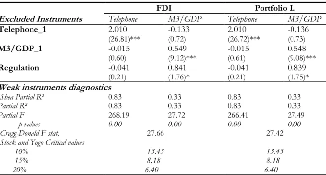
more efficient than the standard fixed effect model (Arellano, 1987) since SUR takes into account the correlation between the errors terms. It is very likely that private capital flows received by a country affect its financial and physical infrastructure development. This potential reverse causality, as explained in the theoretical section, can be a source of endogeneity. In order to solve this problem, which is confirmed by the Nakamura-Nakamura test, we define three instruments: the lagged value of physical infrastructure variable, the lagged value of financial development variable, and the regulation of credit market as financial development variable instrument.10 Instruments diagnostic with
first-stage regressions statistics (partial R², Shea partial R², partial F-test, Cragg-Donald Statistics) reject the hypothesis of weak instruments (table 1).
Table 2.1 First-stage equation
FDI Portfolio I.
Excluded Instruments Telephone M3/GDP Telephone M3/GDP
Telephone_1 2.010 -0.133 2.010 -0.136 (26.81)*** (0.72) (26.72)*** (0.73) M3/GDP_1 -0.015 0.549 -0.015 0.548 (0.60) (9.12)*** (0.61) (9.08)*** Regulation -0.041 0.841 -0.041 0.839 (0.21) (1.76)* (0.21) (1.75)*
Weak instruments diagnostics
Shea Partial R² 0.83 0.33 0.83 0.33
Partial R² 0.83 0.33 0.83 0.33
Partial F 268.19 27.72 266.41 27.49
p-values 0.00 0.00 0.00 0.00
Cragg-Donald F stat. 27.66 27.42
Stock and Yogo Critical values
10% 13.43 13.43
15% 8.18 8.18
20% 6.40 6.40
* significant at 10%; ** significant at 5%; *** significant at 1%
For the estimations, we use three stage least squares (3SLS) which, like two stage least squares (2SLS), deals with the endogeneity problem but also takes into consideration the correlation between the errors terms of the equations like SUR method. Under the null assumption of good specification of all equations in the model, 3SLS is more efficient
10 This variable of credit market regulation indicates governments’ constraints or incentives in term of
control of interest rates on deposits and bank loans. An instrument for financial development, commonly used in the literature is the legal origin. This instrument cannot be used in our case since it is already included in the country fixed effects.
since it deals with the correlation of different equations’ error terms. However, when at least one equation in the system is misspecified, this misspecification extends to all systems by the correlation of error terms, leading to biased and less consistent coefficients. In this case, the 2SLS estimator, although less efficient, is preferable since there is no correlation in error terms and it is consistent, even in the case of the misspecification of one equation in the system. Although results obtained by the 2SLS do not differ significantly (appendix 8), a Hausmann test confirms the preference for 3SLS.
5.3. Results
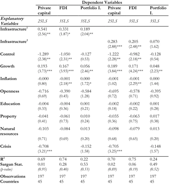
We first consider an index of physical and financial infrastructure obtained with principal components analysis that avoids colinearity problems between infrastructure variables. A second method of aggregation used is the standardisation of variables. This method is similar to principal component analysis but it gives an equivalent weight to each variable in the calculation of the index. The indexes include five variables: the proportion of subscribers of fixed and mobile phone, the electric consumption per capita, the ratio M3/GDP, the credit to private sector, and the deposits in financial institutions. The following table gives the results of estimations with aggregated indexes.
Table 2.2: Estimation with physical and financial infrastructure index Dependent Variables
Private capital
FDI Portfolio I. Private
capital FDI Portfolio I. Explanatory Variables 2SLS 3SLS 3SLS 2SLS 3SLS 3SLS Infrastructure1 0.541 0.331 0.189 (2.56)** (1.87)* (2.04)** Infrastructure2 0.283 0.205 0.070 (2.88)*** (2.48)** (1.62) Control -1.289 -1.050 -0.127 -1.222 -0.982 -0.128 (2.38)** (2.31)** (0.53) (2.28)** (2.18)** (0.54) Growth 0.193 0.167 0.056 0.189 0.171 0.048 (3.73)*** (3.93)*** (2.46)** (3.84)*** (4.24)*** (2.23)** Inflation -0.000 -0.001 0.000 -0.001 -0.001 0.000 (0.80) (2.18)** (1.72)* (1.02) (2.29)** (1.44) Openness -0.716 -0.390 -0.584 -0.695 -0.578 -0.395 (0.69) (0.45) (1.28) (0.72) (0.71) (0.92) Education -0.004 -0.004 0.001 -0.002 -0.002 0.001 (0.33) (0.36) (0.21) (0.18) (0.22) (0.28) Property -0.041 -0.061 0.010 -0.035 -0.063 0.017 (0.41) (0.73) (0.24) (0.36) (0.75) (0.38) Natural resources -0.103 -0.084 0.013 -0.098 -0.079 0.013 (0.71) (0.69) (0.20) (0.68) (0.65) (0.20) Crisis -0.708 -0.152 -0.705 -0.148 (3.21)*** (1.58) (3.25)*** (1.57) R2 0.69 0.74 0.22 0.70 0.75 0.24 Sargan Stat. 0.01 0.28 0.53 0.02 0.06 0.49 (p-value) (0.95) (0.40) (0.53) (0.89) (0.19) (0.52) Observations 197 197 197 197 197 197 Countries 45 45 45 45 45 45 z statistics in parentheses.
All regressions include time and country fixed effects. * significant at 10%; ** significant at 5%; *** significant at 1% 1 Infrastructure index by principal component analysis 2 Infrastructure index by standardization
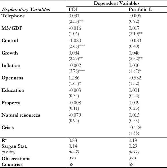
Before interpreting the results obtained with the infrastructure index, we separately estimate the equations with individual variables of infrastructure in order to address criticisms generally made to aggregate indicators that cannot distinguish the partial contribution of each variable. The following table gives the results of estimations considering a proxy for physical infrastructure (the proportion of fixed and mobile phone subscribers) and another one for financial development (M3/GDP) separately.
Table 2.3: Estimation (3SLS) with differentiation of physical and financial infrastructure
Dependent Variables
Explanatory Variables FDI Portfolio I.
Telephone 0.031 -0.006 (2.53)** (0.92) M3/GDP -0.016 0.017 (1.06) (2.10)** Control -1.080 -0.083 (2.65)*** (0.40) Growth 0.084 0.048 (2.29)** (2.52)** Inflation -0.002 0.000 (3.73)*** (1.87)* Openness 1.286 -0.532 (1.65)* (1.32) Education -0.003 0.001 (0.34) (0.22) Property -0.008 0.009 (0.11) (0.23) Natural resources -0.079 0.015 (0.94) (0.35) Crisis -0.128 (1.55) R2 0.88 0.19 Sargan Stat. 0.14 0.29 (p-value) (0.29) (0.41) Observations 239 239 Countries 58 58 z statistics in parentheses.
All regressions include time and country fixed effects. * significant at 10%; ** significant at 5%; *** significant at 1%
Beside the instrument diagnostic tests which reject the hypothesis of weak instruments, the Sargan overidentification test does not reject the validity of the instruments. Control variables have almost identical effects when considering the index of infrastructure or individual variables of infrastructure and financial development. The macroeconomic instability, characterised by a high inflation or a banking crisis negatively affects FDI and portfolio investments respectively (table 2.2). Inflation positively affects portfolio investment. This result could illustrate the fact that Latin American countries, which attract an important part of portfolio investment in the sample, have higher inflation, particularly during the Mexican crisis of 1994. Capital controls11 have a negative effect on
private capital inflows and a good economic performance characterised by a high growth rate positively influences private flows. Countries that are more open also receive more FDI.12
Concerning the two variables of interest, the index of physical and financial infrastructure, either obtained by the principal components analysis or by the standardisation method, positively and significantly affects private capital flows and each of its components (FDI and portfolio investments). Physical and financial infrastructure have a stronger impact on FDI than on portfolio investments, but this result gives no indication of the respective
11 The measure of capital control is the average of proxies of government restrictions that affect capital
mobility (capital account restrictions, current account restrictions, presence of multiple exchange rates and repatriation requirements for export proceeds). There is a structural break in capital account data series in 1996 when the IMF started to report more details on capital account -permitting a measure of the intensity of capital account restriction - instead of the dichotomous variable. That makes the data before and after 1996 not entirely comparable. Quinn (1997) and Mody and Murshid (2005) have constructed single data series using the IMF publications. Chinn (2004) finds also that Quinn index explain 71 percent of the four variables we used to construct our index before 1996. As Mody and Murshid (2005), a robustness check using a truncated sample (before 1996) does not change our results.
12 Education does not affect significantly private capital flows to developing countries. According to the
type of FDI (vertical FDI or horizontal FDI), multinational firms will look for unskilled cheap labor or skilled more expensive labor force. Urata and Kawai (2000) find that skilled labor availability discourages Japanese FDI. After a breakdown analysis, the authors show that skilled labor positively affects FDI in developed countries but the effect is not significant for developing countries.
importance of physical or financial infrastructure in the attractivity of FDI or portfolio investments. Table 2.3 deals with this question by underlining the fact that physical infrastructure only affects FDI inflows while financial infrastructure only has a significant effect on portfolio investments. Indeed, a rise of 1 percentage point in the number of fixed and mobile phone subscribers increases FDI inflows by 0.03 percentage point. This result illustrates the existence of a minimal condition in order to guarantee prosperity of investments and thus attract FDI. A large number of economic activities (especially industrial ones) require a minimum of communication infrastructure (telephone, roads) allowing or facilitating the access to raw and intermediate materials but also the access to markets, reducing production costs. The government usually provides financing for infrastructure since firms can hardly support the cost. The existence of infrastructure thus creates a favourable business environment, encouraging investments, particularly foreign investments.
Portfolio investments are more volatile and relatively scarce in developing countries. Of the two infrastructure variables, only financial development significantly and positively affects portfolio investment flows to developing countries. A rise of 1 percentage point of liquidity liabilities increases portfolio investments by 0.02 percentage point. Inflows of portfolio investments require a high level of financial development since this form of capital flow is most frequently negotiated in stock markets. By improving information sharing, developed financial markets reduces transaction costs and the potential risk taken by investors.13
13 The analysis shows that FDI and portfolio investments are mostly explained by identical determinants.
It is important to pinpoint that some specific determinants of portfolio investments relate to the international economic situation, mainly the international interest rate and growth rate, approximated by those of the developed countries. As mentioned above, these important variables in the determination of portfolio investments are captured by time fixed-effects.
5.4. Robustness check and African specificity
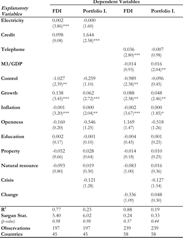
5.4.1. Alternative explanatory variables
The literature suggests several variables that capture the physical infrastructure or financial development of a country. We considered the percentage of subscribers of fixed and mobile phone service in the population as a proxy for physical infrastructure and liquid liabilities (M3/GDP) as a proxy of financial development. The results can be influenced by the choice of these variables. As a robustness check, we estimate the system of equations with electric consumption per capita to reflect physical infrastructure and credit to private sector (in percentage of the GDP) as the financial development variable. The results are robust to the use of these alternative variables (table 2.4).
Table 2.4: Robustness checks (3SLS)
Dependent Variables
Explanatory
Variables FDI Portfolio I. FDI Portfolio I.
Electricity 0.002 -0.000 (3.86)*** (1.60) Credit 0.098 1.644 (0.08) (2.58)*** Telephone 0.036 -0.007 (2.80)*** (0.98) M3/GDP -0.014 0.016 (0.93) (2.04)** Control -1.027 -0.259 -0.989 -0.096 (2.39)** (1.10) (2.38)** (0.45) Growth 0.138 0.062 0.088 0.048 (3.45)*** (2.72)*** (2.38)** (2.46)** Inflation -0.001 0.000 -0.002 0.000 (3.20)*** (2.04)** (3.67)*** (1.85)* Openness -0.160 -0.546 1.169 -0.518 (0.20) (1.25) (1.47) (1.26) Education 0.002 -0.001 -0.004 0.001 (0.17) (0.10) (0.45) (0.25) Property -0.052 0.028 -0.014 0.010 (0.66) (0.64) (0.18) (0.25) Natural resource -0.093 0.019 -0.083 0.016 (0.80) (0.30) (1.00) (0.36) Crisis -0.121 -0.127 (1.28) (1.54) Change -0.336 0.048 (1.09) (0.30) R2 0.77 0.23 0.88 0.19 Sargan Stat. 5.40 6.02 0.24 0.33 (p-value) 0.98 0.98 0.37 0.44 Observations 197 197 239 239 Countries 45 45 58 58 z statistics in parentheses.
All regressions include time and country fixed effects. * significant at 10%; ** significant at 5%; *** significant at 1%
Since portfolio investments are short-term flows, high variability in exchange rates could cause uncertainty in the return on these investments. Exchange rate variability may also negatively affect long-term flows such as FDI by increasing uncertainty in returns. Considering the exchange rate variability variable, the main results remain robust (table 2.4).
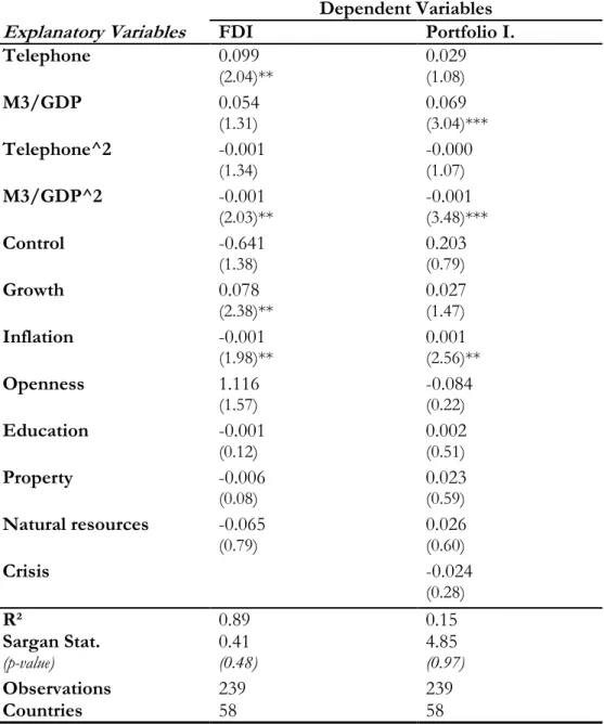
5.4.2. Non-linear relationship
Up to this point, we have only tested linear relations whereas the physical infrastructure may have a congestion effect. Even if the number of subscribers to telephone service or electric consumption per capita has a positive effect on capital inflows, it would be possible that this positive effect vanishes above a certain level of telephone subscribers. For a given level of income, excessive number of telephone subscribers could illustrate high telecommunication cost that forces subscribers to hold one mobile phone for each of the main mobile companies operating in the country. This phenomenon could be observed in African countries such as Côte d’Ivoire or Nigeria. The interaction between infrastructure and other limited factors such as the stock of human capital could also explain the congestion effect. An increase in credit or liquid liabilities can be a signal of a financial development but an excessive supply of money or private credit could also indicate a bad management of the monetary policy or be the precursory sign of a financial crisis. Table 2.5 shows the results considering possible thresholds for the impact of infrastructure and financial development14.
14 The Ramsey-Reset test confirms the non-linearity suspected for the variables of physical and financial
Table 2.5: Non linearity check (3SLS)
Dependent Variables
Explanatory Variables FDI Portfolio I.
Telephone 0.099 0.029 (2.04)** (1.08) M3/GDP 0.054 0.069 (1.31) (3.04)*** Telephone^2 -0.001 -0.000 (1.34) (1.07) M3/GDP^2 -0.001 -0.001 (2.03)** (3.48)*** Control -0.641 0.203 (1.38) (0.79) Growth 0.078 0.027 (2.38)** (1.47) Inflation -0.001 0.001 (1.98)** (2.56)** Openness 1.116 -0.084 (1.57) (0.22) Education -0.001 0.002 (0.12) (0.51) Property -0.006 0.023 (0.08) (0.59) Natural resources -0.065 0.026 (0.79) (0.60) Crisis -0.024 (0.28) R² 0.89 0.15 Sargan Stat. 0.41 4.85 (p-value) (0.48) (0.97) Observations 239 239 Countries 58 58 z statistics in parentheses.
All regressions include time and country fixed effects. * significant at 10%; ** significant at 5%; *** significant at 1%
Telephone^2 and M3/GDP^2 are the squared values of Telephone and M3/GDP
The main results are confirmed and the effects of physical and financial infrastructure on FDI and portfolio investment inflows become higher. Once we have allowed for non-linearity, the results show significant a threshold effect for financial development. This highlights the importance of good management of the monetary policy and the negative impact of excessive money supply.
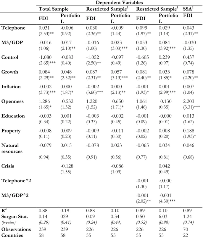
5.4.3. Structural Break and African Specificity
Private capital inflows, particularly FDI to developing countries, have risen exponentially since 1990 with a peak prior to the Asian crisis (chapter 1). Important reforms in the liberalization of current and capital accounts were undertaken by developing countries at the beginning of the 1990s within the framework of the Washington Consensus in order to attract more private capital. A temporal Chow test before and after 1990 enables us to show stability of the coefficients during the two periods. There is no differentiated effect on the determinants of private capital due to the reforms, and no specificity before and after the 1990s crises.15 The analysis of private capital inflows to developing countries also
shows a marginalisation of Sub-Saharan African countries (chapter 1). Analysis of the Sub-Saharan African sample shows an African specificity which is confirmed by the Chow test. Considering only Sub-Saharan African (SSA) countries, the results show that physical infrastructure positively and significantly affects FDI inflows.16
15 Data availability does not allow the test of other dates of potential ruptures or an Andrews-Quandt test
that would enable to determine the break point. The choice of the break period, although imposed to us by the data is also justified theoretically
16 Given the low level of portfolio investment in Sub-Saharan African countries and the fact that South
Africa is the main destination of these portfolio investments, we consider only FDI for the estimation on SSA countries. The specificity of SSA countries is confirmed with the introduction of a dummy in the full sample. The results obtained for the SSA countries sample are similar after a standardization of the coefficients.
Table 2.6: Sub-Saharan Africa specificity (3SLS)
Dependent Variables
Total Sample Restricted Sample1 Restricted Sample1 SSA2
FDI Portfolio I. FDI Portfolio I. FDI Portfolio I. FDI Telephone 0.031 -0.006 0.030 -0.009 0.099 0.029 0.043 (2.53)** (0.92) (2.36)** (1.44) (1.97)** (1.14) (2.31)** M3/GDP -0.016 0.017 -0.016 0.023 0.053 0.084 -0.030 (1.06) (2.10)** (1.00) (3.03)*** (1.30) (3.92)*** (1.35) Control -1.080 -0.083 -1.052 -0.097 -0.605 0.239 0.437 (2.65)*** (0.40) (2.50)** (0.49) (1.26) (0.97) (0.74) Growth 0.084 0.048 0.087 0.057 0.081 0.033 0.078 (2.29)** (2.52)** (2.31)** (3.13)*** (2.40)** (1.85)* (2.20)** Inflation -0.002 0.000 -0.002 0.000 -0.001 0.001 0.007 (3.73)*** (1.87)* (3.60)*** (2.13)** (1.93)* (2.99)*** (1.04) Openness 1.286 -0.532 1.220 -0.650 1.061 -0.130 2.203 (1.65)* (1.32) (1.52) (1.71)* (1.46) (0.35) (3.31)*** Education -0.003 0.001 -0.003 -0.002 -0.001 -0.000 0.013 (0.34) (0.22) (0.33) (0.45) (0.09) (0.01) (1.62) Property -0.008 0.009 -0.009 -0.011 -0.002 0.008 0.188 (0.11) (0.23) (0.11) (0.30) (0.02) (0.20) (1.93)* Natural resources -0.079 0.015 -0.078 0.023 -0.065 0.034 0.046 (0.94) (0.35) (0.91) (0.56) (0.77) (0.81) (0.68) Crisis -0.128 -0.086 0.042 (1.55) (1.09) (0.49) Telephone^2 -0.001 -0.000 (1.30) (1.17) M3/GDP^2 -0.001 -0.001 (2.02)** (4.30)*** R2 0.88 0.19 0.88 0.10 0.89 0.10 0.89 Sargan Stat. 0.14 029 0.09 0.34 0.50 6.03 1.24 (p-value) (0.29) (0.41) (0.24) (0.44) (0.52) (0.98) (0.74) Observations 239 239 226 226 226 226 70 Countries 58 58 55 55 55 55 22 z statistics in parentheses.
All regressions include times and country fixed effects. * significant at 10%; ** significant at 5%; *** significant at 1%
Telephone^2 and M3/GDP^2 are the squared values of Telephone and M3/GDP
1 Restricted sample is the total sample without some major developing countries: Brazil, India and South Africa 2 SSA indicates Sub-Saharan African countries
A rise of 1 percentage points in the number of subscribers to fixed and mobile phone service increases FDI inflows to SSA countries by 0.04 percentage points. These results may be explained by the fact that most SSA countries have a relatively low level of infrastructure development. On average, over the period 1970-2003, only 2 percent of the population in SSA countries were telephone subscribers compared to 5 percent for Asian countries and 12 percent for Latin America countries. A simple simulation shows that if SSA countries were to reach the same level of physical infrastructure development as Asian countries, FDI inflows would increase by 6.5 percentage points. This simulation reveals the importance of physical infrastructure in attracting FDI for SSA countries attractiveness. The estimation for the sub-sample of SSA countries also highlights the importance of trade openness, economic growth and property rights protection in increasing attractiveness for FDI. It is also important to note that the results are robust to potential influential countries (Brazil, India and South Africa) since these countries attract an important part of FDI and portfolio investments received by developing countries.
6. Conclusion
This chapter has analyzed the determinants of private capital flows in developing countries, with particular attention to physical infrastructure and financial development. Based on two theoretical approaches (Lucas paradox and push-pull factors) and after controlling for interaction between components of capital flows (with 3SLS), this study finds that physical infrastructure only fosters FDI inflows while financial development has a positive effect on portfolio investments. The results highlight the importance of non-linearity -particularly for financial development- in analyzing the determinants of foreign private capital. This indicates the importance of sound monetary policy and stronger oversight in the financial system. Indeed, lax monetary policy and excessive credit provision could weaken the financial system and significantly reduce portfolio investment inflows. It is thus important that policies aiming to attract more private capital consider also the possible negative effects such as sudden stops or reversal of short-term capital flows by maintaining an adequate monetary policy and improving the supervision and the regulation of the financial system.
A study of African specificity underlines the important role of physical infrastructure in attracting FDI inflows. Development of infrastructure should attract more private investments, in particular from abroad. Programs such as the NEPAD (New Partnership for Africa’s Development) in Africa aim to find more funds for infrastructure. This study encourages this type of initiative for a continent which should benefit considerably from the development of its infrastructure by attracting private capital, in particular FDI. Beyond their effects on private capital flows, the development of infrastructure also promotes economic growth by increasing the productivity of the economy.
To give more credit to these findings, the next chapter will analyze deeply the determinants of FDI using disaggregated firm-level data in the manufacturing sector.
References
Ahn YS, Adji S, Willett T. 1998. The Effects of Inflation and Exchange Rate Policies on Direct Investment to Developing Countries. International Economic Journal 12(1): 95-104.
Alfaro L, Kalemli-Ozcan S, Vadym V. 2006a. Why doesn’t Capital Flow from Rich to Poor Countries. Forthcoming Review of Economics and Statistics.
Alfaro L, Kalemli-Ozcan S, Vadym V. 2006b. Capital Flows in a Globalized World: The Role of Policies and Institutions. NBER Working Paper No. 11696.
Arellano M. 1987. Computing Robust Standard Errors for Within-group Estimators.
Oxford Bulletin of Economics and Statistics 49(4): 431-434.
Asiedu E. 2002. On the Determinants of Foreign Direct Investment to Developing Countries: Is Africa Different? World Development30(1): 107-119.
Asiedu E. 2006. Foreign Direct Investment in Africa: The Role of Natural Resources, Market Size, Government Policy, Institutions and Political Instability. The World
Economy 29(1): 63-77.
Bénassy-Quéré A, Coupet M, Mayer T. 2007. Institutional Determinants of Foreign Direct Investment. World Economy, 30(2): 764-82.
Bleaney, M., 1993, “Political uncertainty and private investment in South Africa”, CREDIT Research Paper no. 93/15, University of Nottingham.
Blejer M. and Khan M., 1984, “Government Policy and Private Investment in Developing Countries”, IMF Staff Paper Vol31, No 2.
Bohn H., and Tesar L., 1998, “US Portfolio Investment in Asian Capital Markets” in Reuven Glick (ed.) Managing Capital Flows and Exchange Rates, Cambridge University Press.
Calvo G., Leiderman L., and Reinhart C., 1993, “Capital Inflows and The Real Exchange Rate Appreciation in Latin America: The Role of External Factors” IMF Staff
Papers, Vol. 40, No 1.
Calvo G, Leiderman L, Reinhart C. 1996. Inflows of Capital to Developing Countries in the 1990’s. Journal of Economic Perspectives10(2): 123-139.
Carlson M., and Hernández L., 2002, “Determinants and Repercussions of the Composition of Capital Inflows”, Board of Governors of the Federal Reserve System, International Finance Discussion Papers, Number 717.
Chinn M. 2004. The compatibility of capital controls and financial development: a selective survey and
empirical evidence. In: De Brower, G., Wang, Y. (Eds.), Financial Governance in East
Asia: Policy Dialogue, Surveillance, and Cooperation. Routledge, London. pp. 216-238.
Chuhan P., Claessens S., and Mamingi N., 1998, “Equity and Bond Flows to Latin America and Asia: The Role of Global and Country Factors”, Journal of Development
Economics, Vol. 55, 439-463.
Corbo V., and Hernàndez L., 2001, “Private Capital Inflows and the Role of Economic Fundamentals” In Felipe Larrain (ed.), Capital Flows, Capital Controls, and Currency Crisis: Latin America in the 1990s. Michigan University Press.
Coval JD, Moskowitz TJ. 1999. Home Bias at Home: Local Equity Preferences in Domestic Portfolios. Journal of Finance54(6): 2045-2073.
Coval JD, Moskowitz TJ. 2001. The Geography of Investment: Informed Trading and Asset Prices. Journal of Political Economy109(4): 811-841.
Dasgupta D., and Rahta D., 2000, “What Factors Appear to Drive Private Capital Flows to Developing Countries? And How Does Official Lending Respond?”, World
Demurger S., “Infrastructure Development and Economic Growth: An Empirical Investigation,” Journal of Comparative Economics 29 (1) 2001.
Fernandez-Arias E. 1996. The New Wave of Private Capital Inflows: Push or Pull? Journal
of Development Economics48(2): 389-418.
Fernandez-Arias E. Montiel P. 1996. The Surge in Capital Inflows to Developing Countries: An Analytical Overview. World Bank Economic Review10(1): 51-77.
Ferrucci G, Herzberg V, Soussa F, Taylor A. 2004. Understanding Capital Flows to Emerging Market Economies. Financial Stability ReviewJune(16): 89-97.
Gastanaga V, Nugent JB, Pashamova B. 1998. Host Country Reforms and FDI Inflows: How Much Difference Do They Make? World Development26(7): 1299-1314.
Gooptu S., 1994, “Are Portfolio Flows to Emerging Markets Complementary or Competitive?”, World Bank, Policy Research Working Paper No 1360.
Greene J. and Villanueva D., 1991, “Private Investment in Developing Countries: An Empirical Analysis”, IMF Staff Paper 38, No. 1.
Hajivassilou V. 1987. The External Debt Problems of LDC’s: An Econometric Model Based on Panel Data. Journal of Econometrics36(1-2): 205-230.
Hausmann R, Fernandez-Arias E. 2000. Foreign Direct Investment: Good Cholesterol. Inter-American Development Bank Working Paper No. 417.
Hernandez L., Medallo P., and Valdes R., 2001, “Determinants of Private Capital Flows in the 1970s and 1990s: Is there Evidence of Contagion?”, IMF Working Paper 01/64.
Huang Y., 2006, “Private Investment and Financial Development in a Globalized World”, Discussion Paper 06/589, Department of Economics, University of Bristol.
IMF. 2007. Reaping the Benefits of Financial Globalization. (Washington, June 1). Available via the Internet: www.imf.org/external/np/res/docs/2007/0607.htm. IMF. 2008. Regional Economic Outlook, Sub-Saharan Africa. April, Washington, DC.
Available via the Internet:
http://www.imf.org/external/pubs/ft/reo/2008/AFR/eng/sreo0408.pdf
Jenkins C. and Thomas L., 2002, “Foreign Direct Investment in Southern Africa: Determinants, Characteristics and Implications for Economic Growth and Poverty Alleviation”. Mimeo.
Kang S., Kim S., Kim H. S., Wang Y., 2003, “Understanding the Determinants of Capital Flows in Korea: An Empirical Investigation” Mimeo.
Kim Y. 2000. Causes of Capital Flows in Developing Countries. Journal of International
Money and Finance 19(2): 235-253.
Kumar N. 2002. Infrastructure Availability, Foreign Direct Investment Inflows and Their Export-orientation: A Cross-Country Exploration. RIS Discussion Paper No. 26. Levine R. 1997. Financial development and economic growth: views and agenda. Journal of
Economic Literature 35(2): 688-726.
Levine R. 2003. More on finance and growth: More finance more growth. Reserve Bank of
St. Louis Review 85(4): 31-52.
Lopez-Mejia A. 1999. Large Capital Flows: Causes, Consequences and Policy Responses.
Finance and Development 36(3): 28-31.
Loree DW, Guisinger SE. 1995. Policy and Non-Policy Determinants of U.S. Equity Foreign Direct Investment. Journal of International Business Studies 26(2): 281-299. Lucas RE. 1990. Why Doesn’t Capital Flow from Rich to Poor Countries? American
Economic Review 80(2): 92-96.
Perception and Reality. Chapter 2 of Canadian Development Report 2004.
Mody A, Murshid AP. 2005. Growing up with capital flows. Journal of International
Economics65: 249-266.
Mody A, Srinivasan K. 1998. Japanese and United States Firms as Foreign Investors: Do They March to the same Tune? Canadian Journal of Economics31(4): 778-799.
Mody A, Taylor MP, Kim JY. 2001. Modeling Economic Fundamentals for Forecasting Capital Flows to Emerging Markets. International Journal of Finance and Economics
6(3): 201-206.
Mody A., and Taylor M., P., 2004, “International Capital Crunches: The Time-Varying Role of Informational Asymetries”, Royal Economic Society Annual Conference 2004 113, Royal Economic Society.
Montiel P, Reinhart C. 1999. Do Capital Controls and Macroeconomic Policies Influence the Volume and Composition of Capital Flows? Evidence from the 1990s. Journal
of International Money and Finance, 18(4): 619-635.
Montiel P. J., 2006, “Obstacles to Investments in Africa: Explaining the Lucas Paradox”, Presented at the high-level seminar Realizing The Potential for Profitable Investment in Africa.
Morrissey O., 2003, Contribution to Development Report 2003, Finance for Development, Enhancing the role of private finance: Attracting foreign private capital to African countries.
Naudé WA, Krugell WF. 2007. Investigating geography and institutions as determinants of foreign direct investment in Africa using panel data. Applied Economics 39(10): 1223-1233.
Navaretti GB, Venables AJ. 2006. Multinational Firms in the World Economy. Princeton University Press.
Ngowi HP. 2001. Can Africa Increase Its Global Share of Foreign Direct Investment (FDI) West Africa Review2(2): 1-22.
Portes R, Rey H. 2005. The Determinants of Cross-Border Equity Transaction Flows.
Journal of International Economics65(2): 269-296.
Quinn D. 1997. The correlates of change in international financial regulation. American
Political Science Review91(3): 531-551.
Ramamurti R, Doh J. 2004. Rethinking foreign infrastructure investment in developing countries. Journal of World Business 39(2): 151-167.
Reinhart C, Rogoff K. 2004. Serial Default and the “Paradox” of Rich to Poor Capital Flows. American Economic Review94(2): 52-58.
Root F, Ahmed A. 1979. Empirical determinants of manufacturing direct foreign investment in developing countries. Economic Development and Cultural Change 27(4): 751-767.
Sader F. 2000. Attracting Foreign Direct Investment into Infrastructure. Why Is It So Difficult? Occasional PaperNo. 12. Foreign Investment Advisory Service.
Schneider F, Frey B. 1985. Economic and political determinants of foreign direct investment. World Development13(2): 161-175.
Serven L. and Solimano A., 1993, “Debt Crisis, Adjustment Policies and Capital Formation in Developing Countries: Where Do We Stand?”, World Development, Vol.21, No.11, pp. 127-40.
Shaw ES. 1973. Financial Deepening in Economic Development, Oxford University Press, New York.
Temple J., 1999, “The New Growth Evidence”, Journal of Economic Literature, volume 37(1), pp 112-156.
Urata S, Kawai H. 2000. The determinants of the location of foreign direct investment by Japanese small and medium-sized enterprises. Small Business Economics15(2): 79-103. Ying Y, Kim Y. 2001. An Empirical Analysis on Capital Flows: The Case of Korea and
Mexico. Southern Economic Journal67(4): 954-968.
Wheeler D, Mody A. 1992. International Investment Location Decisions: The Case of U.S. Firms. Journal of International Economics33(1-2): 57-76.
Willoughby C., 2003, “Infrastructure and Pro-Poor Growth: Implications of Recent Research”, United Kingdom Department for International Development.
Appendices
Appendix 2.1: List of variables
Variables Definitions Sources
FDI Foreign direct investment, net inflows (% of
GDP) Global Development
Finance (2005)
PORTFOLIO I. Portfolio investment, equity (% of GDP)
DEBT Bank and trade-related lending (% of GDP)
M3/GDP Liquid liabilities (M3) as % of GDP
Financial Structure Dataset (2006)
Credit Domestic credit provided by banking sector (%
of GDP)
Deposit Financial System Deposits (% of GDP)
Telephone Fixed line and mobile phone subscribers per 100
inhabitants
World Development Indicators (2005)
Electricity Electric consumption per capita
Growth Economic growth rate
Inflation Inflation rate
Openness Sum of exports and imports of goods and
services as a share of gross domestic product
Change Exchange rate variability (standard deviation)
Control
Capital control indicator : average of four dummies: Exchange arrangements, payments restrictions on current transactions and on capital transactions, and repatriation requirements for export proceeds Milesi Ferretti (1970-1997) and Annual Report on Exchange Arrangement and Exchange Restrictions (1998-2003)
Crisis Financial crisis dummy Caprio and Klingebel
(2003)
Education Gross primary enrollment rate UNESCO Statistics
(2004)
Natural resources Log of oil, gas, metal and mineral rents World Bank (2002)
Regulation Credit market regulation
Fraser Institue (2005)
Appendix 2.2: Descriptive Statistics
Variable Observation Mean Standard D. Min Max
Private capital 239 1.90 2.77 -3.32 31.72 FDI 239 1.79 2.67 -3.32 31.72 Portfolio I. 239 0.11 0.52 -0.78 5.82 Telephone 239 7.80 11.94 0.06 75.46 Electricity 197 813.87 839.78 26.20 3961.69 M3/GDP 239 36.42 21.39 9.86 124.90 Credit 235 0.46 0.29 0.06 1.57 Deposit 239 29.71 19.84 0.05 116.38 Growth 239 1.13 2.81 -7.89 8.24 Inflation 239 34.13 189.34 -18.78 2414.35 Openness 239 0.62 0.30 0.13 2.16 Control 239 0.61 0.27 0.00 1.00 Education 239 95.49 20.70 25.00 148.67 Property 239 4.46 1.30 1.58 7.06 Natural resources 239 18.99 3.96 7.73 24.33 Crisis 239 0.42 0.49 0.00 1.00 Regulation 239 5.94 2.15 0.00 9.85
Appendix 2.3: Evolution of variables 0 5 1 0 1 5 2 0 T e le p h o n e 1970 1975 1980 1985 1990 1995 2000 Year 4 0 0 6 0 0 8 0 0 1 0 0 0 1 2 0 0 E le c tr ic it y 1970 1975 1980 1985 1990 1995 2000 Year 3 2 3 4 3 6 3 8 4 0 M 3 /P IB 1970 1975 1980 1985 1990 1995 2000 Year .3 6 .3 8 .4 .4 2 .4 4 .4 6 C re d it 1970 1975 1980 1985 1990 1995 2000 Year 2 4 2 6 2 8 3 0 3 2 3 4 D e p o s it 1970 1975 1980 1985 1990 1995 2000 Year 0 1 2 3 G ro w th 1970 1975 1980 1985 1990 1995 2000 Year
0 5 0 1 0 0 1 5 0 In fl a ti o n 1970 1975 1980 1985 1990 1995 2000 Year .4 .5 .6 .7 O p e n n e s s 1970 1975 1980 1985 1990 1995 2000 Year .5 .5 5 .6 .6 5 .7 .7 5 C o n tr o l 1970 1975 1980 1985 1990 1995 2000 Year 8 5 9 0 9 5 1 0 0 E d u c a ti o n 1970 1975 1980 1985 1990 1995 2000 Year 3 .5 4 4 .5 5 P ro p e rt y 1970 1975 1980 1985 1990 1995 2000 Year 1 8 .5 1 9 1 9 .5 2 0 2 0 .5 N a tu ra l re s o u rc e s 1970 1975 1980 1985 1990 1995 2000 Year 0 .2 .4 .6 C ri s is 1970 1975 1980 1985 1990 1995 2000 Year 5 5 .5 6 6 .5 7 R e g u la ti o n 1970 1975 1980 1985 1990 1995 2000 Year
Appendix 2.4: Illustration of Lucas paradox among developing countries
Dependent Variable: Private Capital per capita
Explanatory Variables Fixed Effect 2SLS
GDP per capita 0.065 0.061 (11.68)*** (6.43)*** Constant -5.301 -15.896 (0.46) (0.78) Observations 668 571 Countries 106 106 R² 0.25 0.29 t statistics in parentheses
All regressions include time and country fixed effects. significant at 10%; ** significant at 5%; *** significant at 1%
The regression is based on a large sample of developing countries including the countries retained for the rest of the analysis.
Appendix 2.5: Correlation between the main variables
FDI Portfolio I. Telephone Electricity M3/GDP Credit Deposit
FDI 1 Portfolio I. 0.0812 1 Telephone 0.2401* 0.0587 1 Electricity 0.3146* 0.2042* 0.6613* 1 M3/GDP 0.1080* 0.1006* 0.3543* 0.2998* 1 Credit -0.0276 0.2246* 0.2933* 0.4181* 0.7031* 1 Deposit 0.1849* 0.1408* 0.4365* 0.4170* 0.9506* 0.7109* 1 * significant at 1%
Appendix 2.6: Eigenvalue and variance with principal components analysis
Principal
components Eigenvalue Proportion of variance
Cumulative Variance 1 3.07 0.61 0.61 2 1.19 0.24 0.85 3 0.42 0.09 0.94 4 0.27 0.05 0.99 5 0.05 0.01 1.00 Eigenvectors Variable 1 2 3 4 5 M3/GDP 0.50 -0.36 -0.31 -0.23 0.69 Deposit 0.53 -0.25 -0.26 -0.28 -0.72 Credit 0.47 -0.26 0.60 0.59 -0.01 Telephone 0.34 0.63 -0.49 0.50 0.02 Electricity 0.37 0.59 0.49 -0.52 0.09
Appendix 2.7: 2SLS Estimation with physical and financial infrastructure index Dependent Variables Explanatory Variables Private capital
FDI Portfolio I. Private
capital FDI Portfolio I. Infrastructure1 0.541 0.327 0.191 (2.56)** (1.84)* (2.05)** Infrastructure2 0.283 0.207 0.071 (2.88)*** (2.50)** (1.63) Control -1.289 -1.051 -0.136 -1.222 -0.980 -0.137 (2.38)** (2.31)** (0.57) (2.28)** (2.18)** (0.58) Growth 0.193 0.166 0.054 0.189 0.171 0.046 (3.73)*** (3.92)*** (2.35)** (3.84)*** (4.25)*** (2.12)** Inflation -0.000 -0.001 0.000 -0.001 -0.001 0.000 (0.80) (2.20)** (1.76)* (1.02) (2.28)** (1.48) Openness -0.716 -0.377 -0.564 -0.695 -0.590 -0.373 (0.69) (0.43) (1.24) (0.72) (0.73) (0.87) Education -0.004 -0.004 0.001 -0.002 -0.002 0.001 (0.33) (0.36) (0.18) (0.18) (0.22) (0.26) Property -0.041 -0.061 0.011 -0.035 -0.063 0.017 (0.41) (0.72) (0.25) (0.36) (0.76) (0.40) Natural resources -0.103 -0.084 0.010 -0.098 -0.078 0.010 (0.71) (0.69) (0.16) (0.68) (0.65) (0.16) Crisis -0.708 -0.195 -0.705 -0.192 (3.21)*** (2.01)** (3.25)*** (2.01)** R2 0.84 0.86 0.25 0.84 0.87 0.27 Sargan Stat. 0.01 0.27 0.33 0.02 0.06 0.28 (p-value) 0.95 0.60 0.57 0.89 0.80 0.59 Observations 197 197 197 197 197 197 Countries 45 45 45 45 45 45 z statistics in parentheses.
All regressions include time and country fixed effects. * significant at 10%; ** significant at 5%; *** significant at 1% 1 Infrastructure index by principal component analysis 2 Infrastructure index by standardization.