Metamorphic Code Generation from LLVM IR Bytecode

San Jose State University

SJSU ScholarWorks

Master's Projects Master's Theses and Graduate Research

Spring 2013

Metamorphic Code Generation from LLVM IR

Bytecode

Teja Tamboli

San Jose State University

Follow this and additional works at:https://scholarworks.sjsu.edu/etd_projects

This Master's Project is brought to you for free and open access by the Master's Theses and Graduate Research at SJSU ScholarWorks. It has been accepted for inclusion in Master's Projects by an authorized administrator of SJSU ScholarWorks. For more information, please contact scholarworks@sjsu.edu.

Recommended Citation

Tamboli, Teja, "Metamorphic Code Generation from LLVM IR Bytecode" (2013).Master's Projects. 301. DOI: https://doi.org/10.31979/etd.adyy-u2vw

Metamorphic Code Generation from LLVM IR Bytecode

A Project Presented to

The Faculty of the Department of Computer Science San Jose State University

In Partial Fulfillment

of the Requirements for the Degree Master of Science

by Teja Tamboli

c

2013 Teja Tamboli

The Designated Project Committee Approves the Project Titled

Metamorphic Code Generation from LLVM IR Bytecode

by Teja Tamboli

APPROVED FOR THE DEPARTMENTS OF COMPUTER SCIENCE

SAN JOSE STATE UNIVERSITY

May 2013

Dr. Mark Stamp Department of Computer Science Dr. Robert Chun Department of Computer Science Dr. Sami Khuri Department of Computer Science

ABSTRACT

Metamorphic Code Generation from LLVM IR Bytecode by Teja Tamboli

Metamorphic software changes its internal structure across generations with its functionality remaining unchanged. Metamorphism has been employed by malware writers as a means of evading signature detection and other advanced detection strate-gies. However, code morphing also has potential security benefits, since it increases the “genetic diversity” of software.

In this research, we have created a metamorphic code generator within the LLVM compiler framework. LLVM is a three-phase compiler that supports multiple source languages and target architectures. It uses a common intermediate representation (IR) bytecode in its optimizer. Consequently, any supported high-level programming language can be transformed to this IR bytecode as part of the LLVM compila-tion process. Our metamorphic generator funccompila-tions at the IR bytecode level, which provides many advantages over previously developed metamorphic generators. The morphing techniques that we employ include dead code insertion—where the dead code is actually executed within the morphed code—and subroutine permutation. We have tested the effectiveness of our code morphing using hidden Markov model analysis.

ACKNOWLEDGMENTS

Firstly, I would like to thank Dr. Mark Stamp, my project advisor, for his guid-ance and support throughout my Master’s degree and project.

Secondly, I would like to thank my committee members, Dr. Sami Khuri and Dr. Robert Chun for providing suggestions without which this project would not be possible.

Finally, I would like to thank my family and my husband Onkar Deshpande for their encouragement, motivation, andl support.

TABLE OF CONTENTS CHAPTER 1 Introduction . . . 1 2 Malware . . . 4 2.1 Malware Types . . . 4 2.1.1 Virus . . . 4 2.1.2 Worms . . . 6 2.2 Detection Techniques . . . 7

2.2.1 Signature Based Detection . . . 7

2.2.2 Anomaly Based Detection . . . 7

2.2.3 Hidden Markov Model Based Detection . . . 8

3 Metamorphic Techniques . . . 9

3.1 Register Swap . . . 9

3.2 Subroutine Permutation . . . 9

3.3 Dead Code Insertion . . . 11

3.4 Instruction Substitution . . . 11

3.5 Transposition . . . 12

3.6 Formal Grammar Mutation . . . 12

4 LLVM . . . 15

4.1 Introduction . . . 15

4.2 Architecture of LLVM . . . 15

4.2.2 LLVM Design . . . 16 4.3 LLVM IR Bytecode . . . 18 4.4 Tools in LLVM . . . 20 4.4.1 llvm-gcc (.c → .s) . . . 20 4.4.2 llvm-as (.s → .bc) . . . 21 4.4.3 lli . . . 21 4.4.4 Opt . . . 21 4.4.5 llvm-dis . . . 21 4.4.6 llc . . . 22 4.4.7 llvm-link . . . 22

5 Hidden Markov Models and Virus Detection . . . 23

5.1 HMM . . . 23

5.1.1 Example . . . 25

5.2 The Three Problems . . . 27

5.2.1 Forward Algorithm . . . 29

5.2.2 Backward Algorithm . . . 29

5.2.3 Baum-Welch Algorithm . . . 30

5.3 HMM and Virus Detection . . . 31

5.3.1 Log Likelihood Per Opcode . . . 32

5.3.2 Effectiveness of HMM Detection . . . 33

5.4 Evading HMM Detection . . . 34

6 Design and Implementation . . . 35

6.2 Challenge and Innovation . . . 35

6.3 Goals . . . 36

6.4 Metamorphic Techniques Used . . . 36

6.4.1 Dead Code Insertion . . . 37

6.4.2 Function Permutation . . . 37

6.5 Implementation . . . 38

6.5.1 Dead Code Insertion . . . 38

6.5.2 Call Dead Functions . . . 39

6.5.3 Function Permutation . . . 40 6.6 Software Used . . . 41 7 Experiments . . . 42 7.1 Base File . . . 42 7.2 HMM . . . 44 7.3 Detection . . . 48 8 Conclusion . . . 51 APPENDIX Additional HMM results . . . 58

LIST OF TABLES

1 HMM Notations [43] . . . 24 2 Probabilities of observing (S, M, S, L) for all possible state sequences 28 3 ROC AUC statistics for rate of dead code insertion . . . 47 4 LLVM optimizer passes used to remove dead code . . . 49 A.1 ROC AUC statistics for rate of dead code insertion . . . 60

LIST OF FIGURES

1 Multiple shapes of a metamorphic virus body [21]. . . 6

2 Two different generations of RegSwap [10] . . . 10

3 Subroutine permutation [10] . . . 10

4 Zperm virus [10] . . . 11

5 A simple polymorphic decryptor and two variants [54] . . . 13

6 Formal grammar for decrpyptor mutation [54] . . . 14

7 Three major components of a three-phase compiler . . . 16

8 LLVM design [27] . . . 17

9 LLVM bytecode file format [37] . . . 19

10 Sample C code and its corresponding IR bytecode . . . 19

11 Program’s life cycle in LLVM compiler . . . 20

12 Generic Hidden Markov Model [43] . . . 24

13 HMM Model [43] . . . 26

14 Extracted opcode sequence . . . 32

15 HMM Model . . . 33

16 Metamorphic code generator architecture diagram . . . 38

17 HMM results for base virus and benign files . . . 44

18 HMM results with 10% and 20% dead code insertion . . . 45

19 HMM results with 30% and 50% dead code insertion . . . 46

20 HMM results with rate of dead code insertion . . . 47

22 HMM scores after using optimizers . . . 50

23 HMM scores after using link-time optimizer . . . 50

A.1 HMM results for base virus and benign files . . . 58

A.2 HMM results with 10% and 20% dead code insertion . . . 59

A.3 HMM results with 30% and 50% of dead code insertion . . . 59

CHAPTER 1 Introduction

Software is said to be metamorphic if multiple copies of the same software are structurally different, but functionally equivalent. Examples of such metamorphic code generators can be found at [3, 22, 42].

To date, metamorphic code generation has primarily been used by malware writ-ers, since well-designed metamorphic code can evade signature-based detection and other more advanced detection strategies [22, 42, 53]. However, metamorphism also has the potential to provide security benefits by increasing the “genetic diversity” of software, thereby making several types of attacks more difficult [16, 45].

Well-designed metamorphic malware will evade signature-based detection. Ac-cording to recent research [42, 53], techniques based on hidden Markov models (HMMs) can be used to detect some types of metamorphic malwares.

Many metamorphic malware generators are readily available [51]. Some notable examples include

• G2 (Second Generation virus generator) [52]

• MPCGEN (Mass Code Generator) [51]

• NGVCK (Next Generation Virus Creation Kit) [50]

• VCL32 (Virus Creation Lab for Win32) [5]

In addition, research morphing engines are presented in [22] and [42]. All of these metamorphic generators work at the assembly language level. Note that code

mor-phing of high-level source code is far simpler, but generally ineffective, since such morphing does not provide sufficient control over the resulting executable file.

In this research, we have implemented a metamorphic code generator using the LLVM compiler framework [2]. The LLVM compiler infrastructure provides for compile-time, link-time, run-time, and idle-time optimization of programs written in arbitrary programming languages. It is a three-phase compiler that supports multiple source languages and multiple target architectures. In the optimization process, code is converted to an intermediate representation (IR) bytecode. Our code morphing tool functions at this IR bytecode level, which provides advantages that are some-what analogous to morphing at the source-code level, but also provides the necessary fine-grained control over the resulting executable.

Related research involving LLVM IR bytecode manipulation includes a malware encryption technique implemented as optimizer passes [17]. In addition, in [35], a “shadow attack” is developed using LLVM. This attack hides system call behavior for the purpose of making behavior-based detection of malware more difficult.

We evaluate our morphing technique using the hidden Markov model (HMM) analysis developed in [53] which has been further developed and analyzed in [42, 43]. This body of previous work provides a baseline for determining the effectiveness of our approach.

This paper is organized as follows. In Chapter 2, we provide background infor-mation on computer viruses and detection techniques. Chapter 3 describes generic metamorphic techniques used by metamorphic code generators. Chapter 4 explains the architecture of the LLVM compiler infrastructure and elaborates on IR byte code. Chapter 5 details the design and implementation of the HMM detector used to

evalu-ate our results. Chapter 6 covers the design and implementation of our metamorphic code generator. Experimental results are analyzed in Chapter 7. Chapter 8 contains our conclusion and suggestions for future work.

CHAPTER 2 Malware

Malware is a program developed for performing malicious activities on a com-puter [36]. These malicious activities include crashing disks or operating system or alter system’s data [35]. Writing malware is a challenging task [3] and could be a source of revenue for malware writers. Anti-virus softwares can detect these mali-cious activities and remove them from the computer. To date, most development and research into metamorphic code has involved malware. Therefore, we present background information on malware before turning our attention to the general case of metamorphic code generation.

2.1 Malware Types

There are two most prominent types of malwares: Virus and Worm. They are discussed in details in following subsections.

2.1.1 Virus

Virus-like programs first appeared on microcomputers in the 1980s [8]. Viruses do not have reproductive ability but it can replicate itself. They need human interac-tion to spread the infecinterac-tion from one computer to another. For example, they can get downloaded from Internet or by exchanging infected USB drives or floppy disks. Virus writers constantly develop new obfuscation technique to evade the signature based detection. Most important methods to evade the detection are encryption, polymor-phic and modern metamorpolymor-phic techniques [21]. These techniques are explained in following subsections.

2.1.1.1 Encrypted Viruses

The simplest method to hide the virus body is to encrypt it with different en-cryption keys. Most part of the virus executable is encrypted and a small deen-cryption module exists to decrypt the encrypted body. For example, XORing the key with the virus body [6]. Since the virus is encrypted with different key per infected file, only the decryption module remains constant across generations. There is no common sig-nature in such type of viruses, but virus scanners can detect the decryption module. As a result, the code which encrypts or decrypts, is the part of the signature in most of such virus definitions [13].

2.1.1.2 Polymorphic Viruses

The problem of non-encrypted decryptor module used for detection is solved in these types of viruses. Decryptor module is mutated in each generation. In addition, polymorphic viruses can generate large number of unique decryptors by using different encryption methods. Therefore, not two infections have the same signature [22, 42].

A code emulator is used to detect polymorphic viruses. The emulator emulates decryption process and dynamically decrypts the encrypted virus body [13].

2.1.1.3 Metamorphic Viruses

To avoid detection by emulation, virus writers came up with an advanced tech-nique to write malwares called metamorphism. Metamorphism changes the appear-ance of the virus while keeping its functionality. Metamorphic viruses don’t need encryption or decryption techniques. They produce new virus body on each infec-tion [13].

Metamorphic engine can be kept separate or it can be embedded in the virus. In our implementation, we have kept code generator separate. Some metamorphic techniques are explained in Chapter 3. Figure 1 shows generations of a metamorphic virus whose shape changes but the functionality remains constant.

Figure 1: Multiple shapes of a metamorphic virus body [21].

2.1.2 Worms

Worms are self-replicating malwares. Unlike viruses, they do not need any human intervention to spread. They are standalone [36, 46]. Similar techniques like meta-morphism and polymeta-morphism are used by worms to avoid detection. Worm could be a macro residing in a word document or in a excel sheet which spreads itself across the network. Worms spread from host to host across the network, unlike viruses which only infects executables residing on the host [36, 42].

2.2 Detection Techniques

As a malware evolves, detection mechanisms also evolve. This section elaborates on detection mechanisms employed by anti-virus software.

2.2.1 Signature Based Detection

Signature based detection is a simple and most commonly used technique in anti-virus software. They are popular because of accurate detection, simplicity and speed [44]. In this detection mechanism, scanner scans each executable and looks for specific signatures. Signature consists of sequence of opcodes which uniquely identify the virus. Anti-virus software has database of signatures for different viruses. By comparing the signature, it detects the virus. This technique has to keep on updating database with new malware signatures. Another downside of this type of detection is it cannot detect new virus. Therefore, by using simple code obfuscation techniques, malwares can easily evade the signature based detection [38].

2.2.2 Anomaly Based Detection

The problem of detecting new malwares in signature based detection can be overcome using this type of detection mechanism. Heuristic methods are implemented to detect anomalous behavior. Primarily there are two phases: training and detection. In training, scanner learns normal and malicious behavior e.g. finding root password. After training, it is used to detect malicious activities [44].

Using this technique newbie viruses can be detected but it has downside too [18]. Since its detection is based on how you train the system, it has more number of false positives or false negatives.

2.2.3 Hidden Markov Model Based Detection

Hidden Markov Model (HMM) based virus detection is a comparatively new technique. HMMs are probabilistic models and are widely used in solving problems on pattern recognition. They help in finding the probability of transition from one state to another. HMM has two phases: training and detection. Once you train the model, it can be used to detect benign and malware software [22, 42, 53].

CHAPTER 3 Metamorphic Techniques

The metamorphic code generator described in this paper makes use of morphing techniques like dead code insertion and function permutation. A number of tech-niques include simple technique as register swap to an advanced technique as formal grammar. Some of these techniques are explained in detail in following subsections.

3.1 Register Swap

It is the most simplistic virus. In December 1998, W95/Regswap virus imple-mented metamorphosis via register usage exchange. Register swap means changing the register operands. For example, if instruction isPUSH ECXthen it can be replaced withPUSH EAX. In this technique, opcode sequence remains the same. Figure 2 shows some sample code fragments selected from two different generations of W95/Regswap that use different registers. A wildcard string can be used to detect such type of viruses [10].

3.2 Subroutine Permutation

This technique changes the appearance of a virus by reordering the layout of the virus subroutines. If virus hasnsubroutines, then there can ben! generations without repetition. Some examples are BadBoy and W32/Ghost (discovered in May 2000). BadBoy had 8 subroutines, so 8! = 40,320 (n! = n ∗ (n − 1)!) generations and W32/Ghost had 10 functions, so 10! = 3,628,800 combinations. However, both of them can be detected with search strings as the content of each subroutine remains same [10]. As with register swapping, subroutine permutation is a relatively weak

malware morphing strategy, particularly with respect to statistical based detection. Figure 3 explains this technique.

Figure 2: Two different generations of RegSwap [10]

3.3 Dead Code Insertion

Dead code can be inserted into an existing program. In its simplest form, dead code is never executed. Alternatively, dead code can be executed, provided that it has no effect on the overall program function. Although more difficult, this latter approach is more effective, since the dead code is more difficult to detect.

Dead code can be very effective for evading malware detection, particularly with respect to statistical-based techniques–the dead code can be used to mask the statis-tical properties of the underlying code. By adding such code, a virus can generate infinite number of unique copies. However, dead code insertion can be challenging at the assembly code level, since care must be taken so that addresses remain valid. Win95/Zperm virus appeared in June and September of 2000 incorporated this tech-nique [10]. Figure 4 explains the code structure changes of Zperm-like viruses.

Figure 4: Zperm virus [10]

3.4 Instruction Substitution

In this technique, an instruction is substituted by another equivalent instruction or group of instructions with the same functionality.

For example, MOV R1, R2 can be replaced byPUSH R1and then POP R2. As an-other trivial example XOR R1, R1and SUB R1, R1 both zero the contents of register

R1. But opcode of these two instructions are now different. Instruction substitution is a powerful technique for evading signature detection and altering code statistics. However, instruction substitution is relatively difficult to implement at the assembly code level. The W32/MetaPhor virus is one of the metamorphic virus generators that incorporate the instruction substitution technique [10].

3.5 Transposition

Transposition is reordering the sequence of instructions without changing the actual functionality. It means the sequence can be reordered only if two instructions are independent of each other. For example, instructions:

1. OPCODE [R1] [R2]

2. OPCODE [R3] [R4]

These instructions can be swapped since both instructions are independent of each other. Therefore, they can be reordered with the following sequence without changing the resultant functionality.

1. OPCODE [R3], [R4]

2. OPCODE [R1], [R2]

Similar technique can be applied to group of instructions. As the order of execution itself is different, it is used to evade the signature based detection.

3.6 Formal Grammar Mutation

Formal grammar mutation is a formalization of many existing morphing tech-niques [7, 14, 54]. In general, traditional morphing engines are non-deterministic

automata (NDA), since transitions are possible from every symbol to every other symbol [54]. The symbol set is the set of all possible instructions. It means, any instruction can be followed by any other instruction. By formalizing mutation tech-niques, one can create formal grammar rules and can apply these rules to create viral copies with great variation. Figure 5 shows a simple polymorphic decryptor template and two possible mutations of the decryptor code achieved using the formal gram-mar. Figure 6 With this decryptor template and formal grammar combination, it is possible to generate 960 different decryptors [54].

CHAPTER 4 LLVM

4.1 Introduction

Complexity of modern applications is increasing. They are growing in size, sup-port dynamic upgrades, backups, recovery mechanisms. It is also common to write components in multiple languages to gain efficiency. During the lifetime of the ap-plication, certain components have small hot spots in terms of memory footprint or CPU; other spread their execution time evenly throughout the application. It is im-portant to do program analysis and transformation throughout the lifetime of the application to understand the application behavior.

Lifelong code optimizations include inter-procedural optimizations performed at link-time, machine-dependent optimization at install time, dynamic optimization at run-time and profile-fuided optimization between runs [27, 32].

LLVM (Low Level Virtual Machine) is a compiler infrastructure which has several novel features. It supports language independent instruction set. Each instruction is a Static Single Assignment (SSA). It means each variable is assigned once and then it cannot be reassigned [2, 32]. This is done by using numbers to represent variables. LLVM is part of GCC. It supports static compilation and late compilation from the Intermediate Representation (IR) code similar to Java’s just-in-time (JIT) compiler.

4.2 Architecture of LLVM

The origins of the LLVM infrastructure is in project called “The Lifelong Code Optimization Project” (LCO-Project) which started at the department of computer

science at the university of Illinois at Urbana-Champaign [37].

4.2.1 Traditional Three Phase Compiler Design

Most of the traditional static compilers (For example, GCC used for C/C++ programs) are three-phase compilers. Three main phases includes frontend, optimizer and backend. Figure 7, shows the typical design of three phase compilers [27].

Figure 7: Three major components of a three-phase compiler

The key function of frontend component is to parse the source code, check for any syntactical errors and then build a language specific Abstract Syntax Tree (AST). Optimizers use this tree and transform it to a new representation by applying opti-mization techniques. From AST, it rearranges instructions in order to optimize the code. It removes duplicates, redundant computations. The backend is the machine dependent representation of the code (assembly code). It maps the code to target machine instruction set. Its main goal is to generate correct code that can take advantage of underlying hardware. Common parts of a compiler backend include instruction selection, register allocation, and instruction scheduling [27].

4.2.2 LLVM Design

The key feature of LLVM three-phase compiler design is, it supports multiple frontends and multiple backends by using a common intermediate representation. The frontend can be written in any language which essentially will be converted

to an intermediate representation. This intermediate representation is machine and language independent. A backend can be written for any target platform to compile from this common representation [1, 27]. Figure 8 shows LLVM design.

Figure 8: LLVM design [27]

Using this design it is now easy to add new language by implementing new fron-tend and reusing existing optimizers and backends. New platforms can be supported by implementing new backends. If these components were not separated, then to implement new language we have to start all over from the scratch. To support N

languages and M targets we would need N M different compilers [27].

Another potential advantage of LLVM design is as these components are sepa-rated from each other, skills required to implement frontend are completely different than skills required for implementing backend and optimizer [2, 32]. Frontend person can only maintain or enhance their part of the compiler. This is not the technical issue, but for open source project, it reduces the barrier to contributing as much as possible.

Finally, LLVM design serves broader set of programmers compared to traditional compilers supporting only one source language and target. Traditional open source compilers (like GCC) are stable and efficient because they serve larger communities.

This tends to generate better optimized machine code compared to narrower compilers like Free PASCAL [27].

4.3 LLVM IR Bytecode

The most important aspect of LLVM’s design is to represent optimizer in com-mon intermediate form (IR). This comcom-mon form separates frontend and backend components from each other. It supports lightweight runtime optimizations, cross-function or inter-procedural optimizations, entire program analysis and aggressive restructuring transformations.

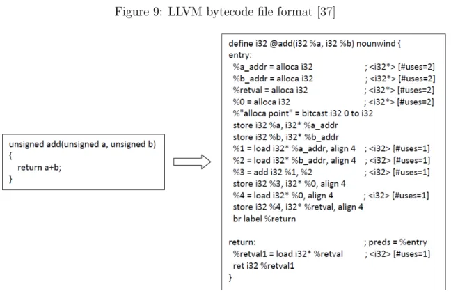
Figure 9 shows the LLVM IR’s structure. It supports following sections [37]:

1. A module: The module is the container which has functions and global variables. 2. Functions: Functions are named, callable units of instructions.

3. Global variables: Global variables which can be accessed by any function.

Figure 10 shows sample C program and its corresponding IR representation.

In LLVM IR, logic is represented in the form of functions. Functions consist of a list of basic blocks. Each basic block consists of a set of instructions. Instructions in basic block are always executed sequentially.

As IR bytecode is the only interface to the optimizer, writing this bytecode is a critical component. It should be easily generated by frontend and should be sufficiently expressive to perform optimizations to convert into real target machine code [27]. Frontend programmers should understand IR and its invariants. LLVM IR has a textual form. Therefore, frontend programmers should output LLVM IR in

Figure 9: LLVM bytecode file format [37]

Figure 10: Sample C code and its corresponding IR bytecode

text. Similarly, backend writers (code generators) should know how to convert it into machine code.

4.4 Tools in LLVM

To compile the program, run optimizations, generate the bytecode or machine code there are various tools available in LLVM infrastructure. Some of these tools are explained in following sections. Program’s life cycle from source program to executable in LLVM compiler is explained in Figure 11.

Figure 11: Program’s life cycle in LLVM compiler

4.4.1 llvm-gcc (.c → .s)

This tool is used to generate the LLVM IR bytecode. It checks for syntacti-cal errors and then produces IR bytecode of the source program. It uses .s or .ll extension [28]. For example,

llvm-gcc -emit-llvm -S hellworld.c

4.4.2 llvm-as (.s → .bc)

This tool is used to generate bitcode file (executable) from the IR bytecode. For example,

llvm-as -f helloworld.s

It creates hellowrold.s.bc file which is target specific executable [29].

4.4.3 lli

To execute LLVM bitcode file, lli command is used [28]. For example, lli helloworld.s.bc

This command executes helloworld program.

4.4.4 Opt

It is used to run different optimizers on IR bytecode. One can write his / her own optimizer on top of inbuilt optimizers. In this project we have written an optimizer pass to call dead code functions. Format of the command is:

opt h optimizer namei h input bytecode or bitcode file i h output bytecode or bitcode file i

For example,

opt -mem2reg hhelloworld.s.bci hmhellow.bci

The file mhellow.bc is generated after running the optimizer pass mem2reg on hel-loworld.s.bc. File mhellow.bc is the optimized executable of the program [28].

4.4.5 llvm-dis

This tool is used to disassemble the LLVM bitcode file to IR bytecode file. llvm-dis -f mhellow.bc -o opthelloworld.s

Using this command we can check how code was optimized in mem2reg pass [29].

4.4.6 llc

This tool is used to generate native assembly-code from bitcode file. For example,

llc -f opthelloworld.bc

A file containing the native assembly code opthelloworld.s is created [28]. Throughout the project we used following command to disassemble the binary.

llc -o file.asm -asm-verbose=0 -march=x86 -x86-asm-syntax=intel -regalloc=default file.bc

Here, file.bc is the input binary file and file.asm is the output file containing assembly code

4.4.7 llvm-link

This tool takes several LLVM bitcode files and links them together and generates a single LLVM bitcode file [33]. For example,

llvm-link -o finalopt.bc addCode.s.bc basic.s.bc

This command generates one finalopt.bc bitcode file after linking addCode.s.bc and basic.s.bc bitcode files.

CHAPTER 5

Hidden Markov Models and Virus Detection

Metamorphism is the best way to evade detection. Recent research proves that Hidden Markov Models (HMMs) are very effective in detecting metamorphic viruses [5, 11, 22, 39, 48, 49, 53]. Hidden Markov models can be viewed as a ma-chine learning technique. In the past, a method is described to train the HMM with sequences of opcodes from viruses which belong to same family [53]. This trained HMM is then used to score binaries, to determine if the given binary belongs to a virus or benign file. Log Likelihood Per Opcode (LLPO) score is calculated and based on this score, threshold is obtained for viruses and benign executables. This thresh-old value categorizes executables between viruses or benign executables based on its LLPO score. The detailed working of HMM and its virus detection mechanism are explained in following sections.

5.1 HMM

The Hidden Markov Model (HMM) is a statistical pattern analysis tool. The notations used in HMM are shown in Table 1 [43]:

As the name suggests, a hidden Markov model includes a “hidden” Markov chain. Although this Markov chain is not directly observable, it is probabilistically related to sequence of observed symbols. A generic Hidden Markov Model is explained in Figure 12. Its state and observation at time t are represented by Xt and Ot respectively. The initial stateX0 andAmatrix together determine the hidden Markov

process. This Markov process is illustrated in Figure 12. Oi is related to the states of Markov process by the matrices A and B.

Table 1: HMM Notations [43]

Symbol Description

T Length of the observed sequence

N Number of states in the model

M Number of distinct observation symbols

O Observation sequence (O0,O1, . . . ,OT−1)

A State transition probability matrix

B Observation probability distribution matrix

π Initial state distribution matrix

Figure 12: Generic Hidden Markov Model [43]

Research in [12] indicates HMMs are used in protein modeling and speech recog-nition systems. HMMs can also be used to detect certain types of software piracy [20]. In general, HMM needs to be trained with the input data. It creates training models based on this training data. Each individual element in the training data is mapped to an observation symbol. All unique observation symbols are then extracted and are represented in the training model. This trained model is then used to determine whether the new sequence of observations is similar to one represented in the training model. HMM collects training data from all known viruses and builds training models one for each family of virus. A new file is tested against these models. If a new file matches with the model, then it can be identified as a virus from that family [43, 53].

5.1.1 Example

Papers [22, 43, 53] explain inner working of HMM with this simple example: Suppose one has to find out the average annual temperature for any given year by observing the tree sizes (S-small,M-medium andL-large). To keep it simple, assume the annual temperature is either hot (H) or cold (C). In addition to this, the prob-ability of annual temperature trend is known. Probprob-ability of a hot year followed by another hot year (HH) is 0.7, a hot year followed by a cold year (HC) is 0.3, a cold year followed by a hot year is 0.4 and a cold year followed by another cold year (CC) is 0.6 [43]. The matrix representation of these probabilities is:

The correlation between tree sizes and temperature is also known. In a hot year, the probability of tree size being small is 0.1, being medium is 0.4 and being large is 0.5. In a cold year, the probability of tree size being small is 0.7, being medium is 0.2 and being large is 0.1 [43]. The matrix representation of this information is as follows:

This known information can be mapped to HMM notations. States are repre-sented by annual temperatures, tree sizes are observable symbols. States H and C

are hidden, as we cannot see the temperature in the past. We have access to see the observation symbols (S, M and L). With this known information, we can build the HMM model described in Figure 13.

Figure 13: HMM Model [43]

Consider we have information of tree size sequence for four consecutive years and it is (S, M, S, L) and by using this information we want to find the annual temper-ature sequences. To solve this problem using HMM, its parameters are explained as follows [43]:

1. State transition probability matrix

A=

0.7 0.3 0.4 0.6

2. The observation probability distribution matrix

B =

0.1 0.4 0.5 0.7 0.2 0.1

3. Number of states (H and C) in the model N = 2.

4. Number of distinct observation symbols (S, M and L)M = 3. 5. Given initial state distribution matrix :

HMM steps to determine transitions of length T = 4 with given observations (S, M, S, L) are as follows [43]:

1. Determine all state transitions which is nothing but NT.

2. Calculate the probability for each state transition (Table 2) with the given observation sequence. For example, the probability of sequence HHCC can be calculated by using following formula:

P(HHCC) = πHbH(S)aH,HbH(M)aH,CbC(S)aC,CbC(L) = (0.6)(0.1)(0.7)(0.4)(0.3)(0.7)(0.6)(0.1) = 0.000212

3. We know that annual temperature sequence will be the one with the highest probability. In Table 2 [43], CCCH has the highest probability so answer is

CCCH sequence.

The brute force method applied here requires exponential amount of work which is infeasible. HMM includes following algorithms to solve three problems.

5.2 The Three Problems

Following three problems can be efficiently solved using HMMs [22, 42, 43]:

Problem 1. The model λ = (A, B, π) and an observation sequence O is known, find P(O |λ).

Problem 2. The model λ = (A, B, π) is known, find an optimal state sequence for the Markov process.

Table 2: Probabilities of observing (S, M, S, L) for all possible state sequences

state sequence probability

HHHH .000412 HHHC .000035 HHCH .000706 HHCC .000212 HCHH .000050 HCHC .000004 HCCH .000302 HCCC .000091 CHHH .001098 CHHC .000094 CHCH .001882 CHCC .000564 CCHH .000470 CCHC .000040 CCCH .002822 CCCC .000847

Problem 3. An observation sequence O, the number of unique symbols M and the

number of states N are known, find the model λ= (A, B, π) that maximizes the probability of O.

First problem concentrates on determining the likelihood of an observation se-quence using the modelλ. Second problem concentrates on exposing the hidden part of the HMM. The third problem concentrates on training the HMM with input obser-vation sequenceOand the parametersM andN. In this paper, we first train a model (Problem 3) on opcode sequences derived from a base piece of software. Then use the trained model to score (Problem 1) morphed versions of this base software. Previous research has shown that HMMs are effective at detecting metamorphic malware, and that HMMs can also be used to detect certain types of software piracy [20]. That is, HMMs have proven useful at detecting morphed or disguised versions of code.

Conse-quently, HMM analysis provides a challenging test for any code morphing technique.

5.2.1 Forward Algorithm

This algorithm or α pass determines P(O |λ) [42, 43]. For t= 0,1, . . . , T −1 and i= 0,1, . . . N−1, define

αt(i) =P(O0,O1, . . . ,Ot, xt=qi|λ)

The probability of the partial observation sequence up to time t is αt(i). Using the forward algorithm, P(O |λ) can be computed as shown below:

1. Let α0(i) = πibi(O0), f ori = 0,1, . . . , N −1

2. For t = 1,2, . . . , T −1 andi= 0,1, . . . N−1, compute [43]

αt(i) = N−1 X j=0 αt−1(j)aij ! bi(Ot) 3. P(O |λ) = N−1 X i=0 αT−1(i) 5.2.2 Backward Algorithm

This algorithm helps to find a most likely optimal state sequence For t= 0,1, . . . , T −1 and i= 0,1, . . . , N −1, define [22, 42, 43]

βt(i) =P(Ot+1,Ot+2, . . . ,OT−1|xt =qi, λ)

Efficiently βt(i) can be calculated in following steps:

2. For t =T −2, T −3, . . . ,0 and i= 0,1, . . . , N −1, compute [43] βt(i) = N−1 X j=0 aijbj(Ot+1)βt+1(j)

Fort = 0,1, . . . , T −2 andi= 0,1, . . . , N −1, define

γt(i) =P(xt=qi|O, λ)

Relevant probability up to timet is measured by αt(i), and after t is measured byβt(i) [43],

γt(i) =

αt(i)βt(i)

P(O|λ)

The most likely state at any time t is the state for which γt(i) is maximum.

5.2.3 Baum-Welch Algorithm

By adjusting the model parameters, this algorithm provides efficient way to best fit the observations. In this algorithm, number of states N and number of unique observation symbolsM are constant. However, other parameters like A,B and π are changeable with row stochastic condition. The process of re-estimating the model is explained below [42, 43]:

1. Initialize λ = (A, B, π) with an approximate guess or random values. For example π= 1/N, Aij = 1/N, Bij = 1/M.

2. Compute αt(i), βt(i), γt(i) and γt(i, j) where γt(i, j) is di-gamma. This Di-gammas can be defined as [42]:

γt(i) =

αt(i)aijbj(Ot+1)βt+1(j)

P(O|λ)

γt(i) and γt(i, j) are related by:

γt(i) = N−1

X

j=0

3. Re-estimate model parameters as : For i= 0,1, . . . , N −1 let

πi =γ0(i)

Fori= 0,1, . . . , N −1 andj = 0,1, . . . , N −1, compute [42]

aij = T−2 X t=0 γt(i, j) ,_T−2 X t=0 γt(i)

Forj = 0,1, . . . , N −1 and k= 0,1, . . . , M −1, compute [42]

bj(k) = X t∈{0,1,...,T−2},Ot=k γt(j) ,_T−2 X t=0 γt(j) 4. If P(O|λ) increases go to step 3

5.3 HMM and Virus Detection

Effectiveness of HMM for metamorphic virus detection is explained in detail in [12, 23]. HMM as a virus detection tool needs to train with the input data to generate training model. Trained HMM, represents the statistical properties of the virus family. These trained models are then used to determine the score of a new binary file. This score indicates how “close” a new binary file is to the virus family that the model represents. Based on threshold values, we can then categorize files.

To train the HMM, first set of virus files belonging to the same family are disas-sembled. From each disassembled file, unique assembly opcodes are extracted. These opcodes constitute the HMM symbols. Example of extracted opcodes is shown in Fig-ure 14. A long observation sequence is generated by concatenating opcode sequences from all virus files within the same family. This concatenated sequence then is used to train an HMM. The set of unique opcodes from this long sequence serve as the set of distinct observation symbols. The example of HMM model is shown in Figure 15.

Figure 14: Extracted opcode sequence

5.3.1 Log Likelihood Per Opcode

In scoring observation sequences to train HMM, product of probabilities needs to be computed. As T increases, product tends to 0 exponentially. To avoid this problem, forward and backward algorithms are used to normalize the result. This process is explained in [43]. log[P(O|λ)] =− T−1 X j=0 logcj

Above equation represents log likelihood. It is sum of log transition probabilities, so log likelihood is length dependent. Longer the sequence, higher will be the log observation probability. The sequence in test set can differ in length comparing to

Figure 15: HMM Model

sequences used to train the HMM. To obtain the LLPO, divide the log likelihood by the number of opcodes in the sequence [53].

5.3.2 Effectiveness of HMM Detection

The effectiveness of HMM in detecting metamorphic virus is proven [53]. Virus files generated by metamorphic code generator NGVCK generate significantly differ-ent files, also got detected by HMM in [53]. The detection rate of HMM is almost

90% [12].

5.4 Evading HMM Detection

Researchers have tried to write the metamorphic engine to evade HMM detec-tion [22]. The dead code is inserted into the virus files based on dynamic scoring algorithm. The block of dead code is inserted into the virus file only if doing so increases the likelihood of virus file score getting closer to the score of benign files.

Results in [23] indicate inserting long sequence of opcodes, like subroutines are more effective in avoiding HMM detection than randomly inserting blocks of dead code. The HMM detector failed when 35% of dead blocks and 30% subroutines were inserted from benign files to virus file. The metamorphic code generator presented in this paper makes use of these results while inserting dead code.

CHAPTER 6

Design and Implementation

6.1 Introduction

Some of the metamorphic techniques explained in Chapter 3 are implemented at IR bytecode level instead of at assembly code. It has been seen in the past that conditional code obfuscation techniques are implemented at IR bytecode level by writing LLVM optimizer passes [17]. Malware writers have also tried to implement “shadow attack” in [35].

The aim of the project is to produce multiple base software copies that are hard to detect and significantly different from each other. When a program is compiled with this optimizer, it generates significantly different morphed copy of the base software. Even after implementing all metamorphic techniques, HMM detector developed in [53] is able to classify virus files and benign files correctly. An unsuccessful attempt was made [11] to escape from HMM-based detector. This proves HMM is very effective in detection. Therefore, our aim is to write metamorphic code generator that evades HMM based virus detector.

6.2 Challenge and Innovation

Morphing code at IR level offers following advantages [2]. These advantages include

• LLVM was originally implemented for C and C++, but its language-agnostic design has spawned a wide variety of front ends which include Objective-C, FORTRAN, Ada, Haskell, Java bytecode, Python, Ruby, Action Script, GLSL,

D, and Rust. Code written in any of the above language can use our code generator to produce metamorphic copies.

• The intermediate form is platform independent.

• At IR level, virtual addresses are not assigned. Addresses get assigned at bitcode level. So, by morphing at IR level, we avoid difficulties associated with morphing at the assembly level.

6.3 Goals

Morphed copies of code should have same functionality as base file. In addition, the higher the percentage of inserted or modified code, the more the morphed files should differ (on average) from the base file. A morphed base file will look like a morphing file, if its opcode counts and opcode sequences are more like morphing files than base file. As previously mentioned, HMMs have a proven record of being able to effective “see through” metamorphic cide. Consequently, if we can morph code sufficiently to confuse HMM-based analysis this will provide a strong indication of the success of our morphing strategy.

6.4 Metamorphic Techniques Used

As we are morphing at IR bytecode level, it is difficult to adopt some of the techniques described in Chapter 3. For example, register swapping and equivalent in-struction substitution are relatively difficult to implement at the IR level. Therefore, to provide a proof of concept, we have restricted our code morphing to a combination of dead code insertion and subroutine permutation. We accomplish both of these morphing strategies by inserting randomy selected complete subroutines of dead code from other program files. In addition, the order of these dead subroutines is

ran-domized. In this way, we create a singnificant amount of transposition and dead variation between different morphed copies. In addition, we insert call statements to all dead code subroutines so that they are not trivially identifiable as dead code. These techniques are discussed in following sections:

6.4.1 Dead Code Insertion

Dead code insertion involves inserting instructions whose result is never used in any other computation. The main goal of adding this code is to increase the diversity of opcodes. Since, we are implementing it at IR bytecode level which has RISC like instruction set; it is difficult to add dead instructions. However, functions can be easily inserted by using linker tool llvm-link. To insert dead code we need IR bytecode of morphing files.

We have used core-util Linux command files [24] and files from httpd web browser [4] to insert the dead code. These files include system level code to do operations that we would expect to be somewhat similar to our selected base code. A detailed algorithm is explained in Section $6.5.1.

LLVM provides options to optimize and remove dead code. Anti-virus softwares are also smart enough to identify code snippets which are not actually getting ex-ecuted. They can track to execution sequence and detect the virus. To make the metamorphic code generator smarter, we “call” the inserted dead code. A detailed algorithm is explained in Section $6.5.2.

6.4.2 Function Permutation

As explained in Chapter 3, function permutation is reordering the layout of function definitions. Since IR bytecode is in the textual form, function permutations

can be implemented easily by changing the sequence of the functions. This helps to evade any pattern matching detector. We have written Python script to operate on IR bytecode and produce another text file which has same functions but with a different layout. A detailed algorithm is explained in Section $6.5.3

6.5 Implementation

In this project we have developed three passes. These passes and their algorithms are explained in following subsections. The high level architecture of our morphing engine appears in Figure 16.

Figure 16: Metamorphic code generator architecture diagram

6.5.1 Dead Code Insertion

First pass operates on inserting the dead code. A base file, a morphing file (i.e., our source of dead code), and a dead code percentage are specified. Based on the percentage of dead code, we determine total number of lines we want to insert

into the base file. We then select complete functions from the morphing file so that the total size approximates the number of lines we want to insert into the base file. These subroutines are integrated into the base file at the linking stage. In the output it provides function names it has inserted. It also distinguishes the output dead function names which can be called in pass 2. The details of this first pass of our code morping techniques are given below.

1. Compile selected morphing file using llvm-gcc command and generate its IR bytecode.

2. From this IR bytecode, determine the function dependencies. 3. For each function, calculate its number of lines.

4. Based on total number of dead code lines, use a greedy strategy to determine a subset of functions which best approximates the number of lines to be inserted. 5. Copy selected functions to a temporary IR bytecode file.

6. Create bitcode files for the base code and temporary IR bytecode usingllvm-as. 7. Merge these two files (using llvm-link).

8. If there are any subrouttine naming conflicts, replace each offending name in the temporary IR bytecode file with a random string. Goto 7.

9. Delete the temporary IR bytecode file.

6.5.2 Call Dead Functions

In this pass, we use the LLVM optimizer to insert a “call” instruction for each dead code subroutine. As mentioned in Section $6.5.1, pass 1 identifies dead functions

which can be called using this pass. The optimizer takes function name as input. It then finds themainfunction definition in the IR bytecode and inserts a “call” type of instruction after every “load” type of instruction. This optimizer operates on Module class. The current implementation does not support structure type of parameters and pointers except single pointers. For each dead code subroutine, we perform the following steps.

1. Find the “function” object of the mainfunction.

2. Iterate over instructions in the function object. If an instruction is of type “load”, then insert the “call” instruction.

3. To insert the “call” instruction, iterate over its function parameters. For each parameter, allocate memory and initialize with a random value.

4. Finally, insert a “call” instruction.

6.5.3 Function Permutation

Third pass performs function permutations by simply reordering functions in the IR bytecode file. This pass is written in python script. Its algorithm is explained in following steps.

1. Read IR bytecode file.

2. Write all global variables in temporary file.

3. By using random class generator, generate random number between 1 to total number of functions.

4. If function is not already added, then write this function definition in temporary IR bytecode file.

5. Repeat steps from 3 until all functions are written to temporary bytecode file.

6.6 Software Used

LLVM 3.1 version source code [34] is used. LLVM commands from this version are used to link and compile the code. LLVM-GCC version 4.2 which comes with MAC operating system is used to create IR bytecode files of the source program.

CHAPTER 7 Experiments

In this section, we use the HMM technique developed in [53] to test the effective-ness of our LLVM-based metamorphic code generator. We add increasing percentages of dead code to find the threshold at which HMM detector starts to fail. We show that after adding about 20% (or more) dead code, our metamorphic code generator started to escape HMM-based detection. These results indicate that our LLVM-based morph-ing strategy is more effective than any of the hacker-produced metamorphic malware generators considered in previous research [53], and is at least as effective as an ex-perimental metamorphic malware generator that was designed specifically to evade HMM-based detection [42].

7.1 Base File

For the experiments given here, we use spike fuzzer [41] as our base software. Fuzzing is a process of sending malformed data to an application to generate failures or errors in the application [19]. Fuzzing finds bugs which can then be used by attackers to run their own code. Fuzzing is one of the best ways in which exploitable software bugs are discovered [15, 19, 40].

As this metamorphic code generator is written within the LLVM compiler, it has different executable format. To disassemble the binary, we cannot use standard tools like IDA-PRO. The base software and morphing files should be disassembled by using the same disassembler.

different morphing files. The morphing files were randomly selected from coreutil Linux command files [10].

Once the morphed files are generated, we use an HMM scoring technique similar to that in [53]. Previous research [22, 42, 53], has consistently shown that the number of hidden states in the HMM does not impact the quality of the file classification. Consequently, we only consider HMMs with N = 2 hidden states. Additional results with N = 3 are presented in Appendix.

First, we train an HMM to model the base file. To obtain sufficient observations for training, we generated 50 copies of the base file, each having a 5% rate of morphing. We used random 50 files as morphing files to create set of files. We then trained an HMM on these 50 morphed files. We refer to this model as the “base HMM”. As discussed in [53], the purpose of the morphing at this stage is simply to prevent the base HMM from overfitting the available data in the base file. Consequently, we use a minimal amount of morphing at this step.

Once base files, morphing files and model are ready, next we use the base HMM model to score 50 morphing fies. Specifically, we score the coreutil Linux commands files which will be used as morphing files in experiments.

If the score of the morphing file is not higher than the base file, then HMM detects it as family of base file. There is a threshold value which determines if the given file is a base (score greater than the threshold) or morphing file (score lower than the threshold). If score of the morphing file is greater than the score of some of base files, then HMM does not have a good threshold which can be used to determine the new file. Thus, some base files can escape the HMM based detection.

morphing files is lower than base files. Thus, the base files generated using our code generator with maximum of 5% are detectable by HMM detector.

Figure 17: HMM results for base virus and benign files

7.2 HMM

We then conducted experiments where we morph the base file at each of the following rates: 10%, 20%, 30%, and finally, 50%. In each case, we generated 50 morphed versions of the base file, with each file morphed at the given rate. These morphed copies were then scored using the base HMM and these scores were compared to the scores obtained for the morphing files. Note that all scores are normalized to a per opcode basis so that file size does not affect the results. By calculating scores at various percentages, we found at which percentage base files start escaping from HMM detection.

lines in IR bytecode of base file.

First graph in Figure 18 shows scores after inserting 10% of dead code. Second graph in Figure 18 shows the result after inserting 20% of dead code.

Figure 18: HMM results with 10% and 20% dead code insertion

After inserting 10% of dead code (left figure) scores of the base morphed files improved a little but still most of the files have scores similar to base files. After inserting 20% (right figure), scores are better but still some files have scores similar to base files.

First graph in Figure 19 shows the result after inserting 30% of dead code. Second graph in Figure 19 shows the results of scores after inserting 50% of dead code.

Results of the scores are significantly improved after inserting 30% and 50% of dead code. For 50% almost all base morphed files have scores almost same as that of morphing files. Increase in percentage of dead code causes improvements in LLPO scores.

Figure 19: HMM results with 30% and 50% dead code insertion

From these results, we see that after inserting 20% dead code, the scores are starting to merge, which indicates that the morphed base files are difficult for the HMM to distinguish from the morphing files. This is precisely the effect that we hope to achieve through code morphing.

Graph in Figure 20, gives overall picture of various percentage of dead code insertions.

Results of Figure 20 are summarized in the ROC curves in Figure 21. These ROC curves plot the false positive rate versus the true positive rate as the threshold is varied throughout the score range [9].

The area under the ROC curve (AUC) is equal to the probability that a classiffier ranks a randomly chosen positive instance higher than a randomly chosen negative one [9]. The AUC values for the ROC curves in Figure 21 are given in the Table 3. Note that an AUC of 1.0 indicates ideal separation (i.e., no false positives or false

Figure 20: HMM results with rate of dead code insertion

negatives), while an AUC of 0.5 indicates that the classiffier yields results that are no better than flipping a coin. After inserting 20% dead code, our HMM classiffier does poorly, and at higher morphing rates, the rate of classification failure increases dramatically. Again, these results show that our code morphing technique is highly effective, at least with respect to this HMM classifier.

Table 3: ROC AUC statistics for rate of dead code insertion

Dead code insertion rate in % AUC

10 1.000

20 0.87080

30 0.77240

Figure 21: ROC curves for rate of dead code insertion

7.3 Detection

There are number of dead code removal optimizers already developed in LLVM. We then conducted experiments to check an effect of these optimizers on our meta-morphic code generator. We conducted two experiments. In the first experiment we used compile-time optimizer options in the order explained in Table 4 to remvoe dead code. All these optimizers perform single pass over the function to remove instructions which are dead [26].

Table 4: LLVM optimizer passes used to remove dead code

LLVM optimizer options Description

O3 Optimization level 3

adce Aggressive Dead Code Elimination

die Dead Instruction Elimination

dce Dead Code Elimination

dse Dead Store Elimination

strip-dead-prototypes Strip Unused Function Prototypes

globaldce Dead Global Elimination

globalopt Global Variable Optimizer

tailcallelim Tail Call Elimination

std-compile-opts Include the standard compile time optimizations

After executing these optimizers on base morphed files with 50% of dead code insertion, we found that they have removed some amount of dead code from base morphed files. But, while optimizing they have used different instructions and so the opcodes. From the Figure 22 we can see that, score of some files is actually improved after using these optimizers.

In the second experiment, we used std-link-opts LLVM link-time optimizer (LTO) to remove dead code. This optimzer as explained in [31] works in multiple phases and very effectively optimizes the code. After executing this optimizer, we found that it has removed all dead code we have inserted and it has also optimized the original base file. Current implementation is not using result of dead functions in the rest of the calculation, therefore it figures out dead functions in its multiple passes and optimizes the code. From the Figure 23 we can see that all 50 files have same HMM score after using this optimizer pass.

After using link-time optimizer our metamorphic code generator becomes inef-fective. All morphed files fall back to the original base file.

Figure 22: HMM scores after using optimizers

CHAPTER 8 Conclusion

In this paper, we presented and analyzed a novel code morphing technique based on LLVM IR bytecode. Our approach makes a strong code morphing engine available as a compile-time option, and requires no special effort on the part of the software developer. As far as we are aware, this is the first general purpose code morphing tool of its kind.

Our metamorphic generator uses dead code insertion and function permutation. The dead code is in the form of functions copied from other programs, and these dead functions are called within the program unlike in [23, 42], which makes their detection and removal more challenging. We tested the effectiveness of our code morphing using an HMM technique that has proven successful in metamorphic malware detection and certain cases of software piracy. We showed that our morphing is highly effective, in the sense that the HMM cannot effectively distinguish our morphed code from other code, even at relatively low morphing rates.

Results from the experiments show that with the increase in rate of dead code insertion, base files starts looking more like morphing files. The Log Likelihood score per opcode of base files and that of morphing files started looking similar to each other.

The HMM detector’s performance is acceptable with 20% of dead code insertion. After inserting, more than 20% of dead code, HMM started misclassifying files, as indicated in ROC curve Figure 21.

opti-mizers to remove dead code from base morphed files. However, after using link-time optimzer it becomes ineffective. All morphed files fall back to the original base file.

There are many possible improvements to the metamorphic generator presented here. The dead code insertion could be improved by making it not depend on complete subroutines it should be possible to do such insertion at the level of basic blocks. Other powerful morphing techniques, such as instruction substitution, could be included. It would also be interesting to employ formal grammar mutation as a framework for implementing the morphing. Additional user control of morphing (via compile-time flags) would be valuable. Finally, improvements in the LLVM infrastructure would serve to make our code morphing techniques more robust. For example, in our current implementation, tools available within the LLVM framework could be used to analyze the morphed bitcode. However, if the bitcode is converted to, say, a Windows PE file, then the tools within LLVM will not be available for such analysis.

Current implementation becomes ineffective after using LLVM link-time opti-mizer as shown in Figure 23. The future work can be done to handle this situation.

LLVM compiler infrastructure can also be used to write complex malwares [17, 35]. More research needs to be done in this area.

LLVM compiler architecture is also useful in detection of viruses. Multiple opti-mizers already exist to remove dead code at IR byte code level [25]. Similar optiopti-mizers can be written to remove other obfuscation techniques.

We used HMM based detector to evaluate the effectiveness. It is seen that it was not able to detect all virus files generated by our code generator. Further research needs to be done to enhance HMM detector. One possible way is to remove dead code first from virus files before computing HMM score.

LIST OF REFERENCES

[1] V. Adve and C. Lattner. A compilation framework for lifelong program analysis and transformation. Proceedings of the 2004 International Symposium on Code

Generation and Optimization, 2004.

http://www.cgo.org/cgo2004/papers/06_76_lattner_c.pdf

[2] V. Adve and C. Lattner. Architecture for a next Generation GCC. First GCC

Annual Developer’s Summit, May 2003.

http://llvm.org/pubs/2003-05-01-GCCSummit2003pres.pdf

[3] An example of metamorphic virus.

http://spth.virii.lu/main.html

[4] Apache httpd web browser source code.

http://www.apache.org/dev/version-control.html

[5] S. Attaluri, S. McGhee, and M. Stamp. Profile hidden markov models and meta-morphic virus detection. Journal in Computer Virology, 5:151–169, 2009.

[6] J. Aycock.Computer Viruses and Malware (Advances in Information Security). Springer-Verlag, New York (2006).

[7] P. Beaucamps. Advanced Metamorphic Techniques in Computer Viruses. Inter-national Conference on Computer, Electrical, and Systems Science, and Engi-neering - CESSE’07, Venice, Italy, 2007.

[8] J. Borello and L. Me. Code Obfuscation Techniques for Metamorphic Viruses, 2008.

http://www.springerlink.com/content/233883w3r2652537

[9] A. P. Bradley. The use of the area under the roc curve in the evaluation of machine learning algorithms. Pattern Recognition, 30:1145–1159, 1997.

[10] Computer virus creation kit.

http://www.informit.com/articles/article.aspx?p=366890&seqNum=6

[11] P. Desai. Towards an Undetectable Computer Virus (2008). Master’s Projects. Paper 90.

http://scholarworks.sjsu.edu/etd_projects/90

[12] FASM.

[13] E. Filiol. Computer viruses: from theory to applications, Volume 1. Birkhauser, 2005, pp. 19–38.

[14] E. Filiol. Metamorphism, formal grammars and undecidable code mutation. In-ternational Journal of Computer Science, 2:70–75, 2007.

[15] Fuzzing on Open Web Application Security project.

https://www.owasp.org/index.php/Fuzzing#File_format_fuzzing

[16] X. Gao and M. Stamp. Metamorphic software for buffer overflow mitigation. Pro-ceedings of 3rd Conference on Computer Science and its Applications, P. P. Dey and M. N. Amin, editors, San Diego, California, June 30, 2005

[17] J. Giffin, M. Sharif, A. Lanzi and W. Lee. Impending

Malware analysis using Conditional Code Obfuscation.

Col-lege of Computing, Georgia Institute of Technology, USA.

http://cyber4.us/sites/default/files/Impeding%20Malware%20Analysis %20Using%20Conditional%20Code%20Obfuscation-NDSS2008.pdf

[18] N. Idika and A.P. Mathur. A Survey of Malware Detection Techniques. Purdue University, p. 48, 2007.

http://www.serc.net/system/files/SERC-TR-286.pdf

[19] Introduction to fuzzing using spike fuzzer.

http://resources.infosecinstitute.com/intro-to-fuzzing/

[20] S. Kazi and M. Stamp. Hidden Markov models for software piracy detection, to appear in Information Security Journal: A Global Perspective

[21] A. Lakhotia. Are Metamorphic Viruses Really Invincible? Virus Bulletin, De-cember 2004.

http://www.iscas2007.org/~arun/papers/invincible-complete.pdf

[22] D. Lin and M. Stamp. Hunting for undetectable metamorphic viruses. Journel

in Computer Virology, 7:201–214, Aug. 2011.

[23] D. Lin. Hunting for undetectable metamorphic viruses (2009).Master’s Projects. Paper 18.

http://scholarworks.sjsu.edu/etd_projects/18

[24] Linux coreutils source code.

http://ftp.gnu.org/gnu/coreutil

[25] List of LLVM Optimizer passes.

[26] LLVM Analysis and Transform passes.

http://llvm.org/docs/Passes.html#id63

[27] LLVM Architecture.

http://www.aosabook.org/en/llvm.html

[28] LLVM command guide tool.

http://llvm.org/docs/CommandGuide/

[29] LLVM Helloworld in C, Overview on LLVM tools and explains how to compile code using LLVM.

http://projects.prabir.me/compiler/wiki/LLVMHelloworldInC.ashx

[30] LLVM IR bytecode format.

http://llvm.org/releases/1.3/docs/BytecodeFormat.html

[31] LLVM Link Time Optimization.

http://llvm.org/docs/LinkTimeOptimization.html

[32] LLVM Programming manual.

http://llvm.org/docs/ProgrammersManual.html

[33] llvm-link tool manual page.

http://llvm.org/docs/CommandGuide/llvm-link.html

[34] LLVM source code.

http://llvm.org/releases/download.html

[35] W. Ma, P. Duan, S. Liu, G. Gu and J. Liu. Shadow Attacks: Automatically evading system-call behavior. Master’s report, Department of Computer Science

and Engineering, Texas A and M University.

http://faculty.cs.tamu.edu/guofei/paper/ShadowAttacks_final-onecolumn.pdf

[36] Panda Security (n.d.), Virus, worms, trojans and backdoors: Other harmful relatives of viruses, 2011.

http://www.pandasecurity.com/homeusers-cms3/security-info/about-malware/ generalconcepts/concept-2.html

[37] J. Praher. A change framework based on the Low Level Virtual Machine Compiler Infrastructure.Thesis report at the Johannes Kepler University Linz, April 2007.

http://llvm.cs.uiuc.edu/pubs/2007-04-PraherMSThesis.pdf

[38] S. Priyadarshi. Metamorphic Detection via Emulation (2011).Master’s Projects. Paper 177.

[39] N. Runwal, R. M. Low, and M. Stamp. Opcode graph similarity and metamorphic detection. Journal in Computer Virology, 8: 37–52, 2012.

[40] Spike fuzzer creation kit.

cryptocity.squarespace.com/files/fuzzing/spike/using_spike.pdf

[41] Spike fuzzer source code.

http://www.immunitysec.com/resources-freesoftware.shtml

[42] S. Sridhara. Metamorphic Worm that Carries Its Own Morphing Engine (2012). Master’s Projects. Paper 240.

http://scholarworks.sjsu.edu/etd_projects/240/

[43] M. Stamp. A revealing introduction to hidden markov models, 2012.

http://www.cs.sjsu.edu/~stamp/RUA/HMM.pdf

[44] M. Stamp. Information Security: Principles and Practice, second edition, Wi-ley, 2011.

[45] M. Stamp. Risks of Monoculture. Inside Risks 165, CACM 47, 3, March 2004.

http://www.csl.sri.com/users/neumann/insiderisks04.html#165

[46] Symantec. What is the difference between viruses, worms, and Trojans?, 2006.

http://service1.symantec.com/support/nav.nsf/docid/1999041209131106

[47] The Lifelong Code Optimization Project. WWW page, 2006.

http://www-faculty.cs.uiuc.edu/~vadve/lcoproject.html

[48] S. Venkatachalam. Detecting undetectable computer viruses (2010). Master’s Projects. Paper 156.

http://scholarworks.sjsu.edu/etd_projects/156

[49] A. Venkatesan. Code obfuscation and virus detection (2008). Master’s Projects. Paper 116.

http://scholarworks.sjsu.edu/etd_projects/116

[50] Virus Construction Kits.

http://computervirus.uw.hu/ch07lev1sec7.html

[51] Virus Creation Tools, VX Heavens.

http://oktridarmadi.blogspot.com/2009/09/ virus-creation-tools-vx-heavens.html

[52] VX Heavens.

http://download.adamas.ai/dlbase/Stuff/VX%20Heavens %20Library/static/vdat/creatrs1.htm

[53] W. Wong and M. Stamp. Hunting for metamorphic engines.Journal in Computer Virology, 2(3):211–229, 2006.

[54] P. Zbitskiy. Code mutation techniques by means of formal grammars and au-tomatons. Journal in Computer Virology, 5:199–207, 2009.

APPENDIX

Additional HMM results

• HMM parameters: N = 3

• Graph base files and morphing files: Figure A.1

Figure A.1: HMM results for base and morphing files

• Graph of dead code insertion = 10%: Figure A.2.a

• Graph of dead code insertion = 20%: Figure A.2.b

• Graph of dead code insertion = 30%: Figure A.3.a

• Graph of dead code insertion = 50%: Figure A.3.b