Short term load forecasting and the effect of
temperature at the low voltage level
Stephen Habena,∗, Georgios Giasemidisb, Florian Zielc, Siddharth Aroraa,d,e
aMathematical Institute, University of Oxford, UK bCountingLab Ltd. & CMoHB, University of Reading, UK cFaculty of Economics, University Duisburg-Essen, Germany
dSa¨ıd Business School, University of Oxford, UK eSomerville College, University of Oxford, UK
Abstract
Short term load forecasts will play a key role in the implementation of smart electricity grids. They are required to optimise a wide range of potential net-work solutions on the low voltage (LV) grid, including integrating low carbon technologies (such as photovoltaics) and utilising battery storage devices. De-spite the need for accurate LV level load forecasts much of the literature has focused on the individual household or building level using data from smart me-ters or on aggregates of such data. In this study we provide detailed analysis of several state-of-the-art methods for both point and probabilistic LV load fore-casts. We evaluate the out-of-sample forecast accuracy of these methodologies on 100 real LV feeders, for horizons from one to four days ahead. In addition, we also test the effect of temperature (both actual and forecast) on the accuracy of load forecasts. We present some important results on the drivers of forecasts accuracy as well as the empirical comparison of point and probabilistic forecast measures.
Keywords: probabilistic load forecasting, low voltage networks, temperature effects, short term load forecasting
∗Corresponding author
1. Introduction
Increased monitoring of the electricity distribution network through ad-vanced metering infrastructures (such as smart meters and substation moni-toring) is providing enhanced visibility and new opportunities for managing and planning the demand on the low voltage (LV) networks. This is particu-5
larly desirable for distribution network operators (DNOs) who must prepare for the increased network stressors and distributed generation as we move to a low carbon economy. Accurate load forecasts can facilitate the management of LV networks in a number of ways including: demand side response [1], storage con-trol [2, 3], energy management systems [4, 5] and integrating distributed energy 10
resources [6].
Low voltage networks are typically the final steps in the distribution elec-tricity network that deliver electrical energy directly to the final customer. In the UK, and many distribution networks around the world, the final 230-240V substations contain between 1 to 6 feeders and supply electricity to between 15
1 and 150 customers [7]. It is worth noting that feeders are particularly het-erogeneous, connected to a diverse mix of domestic customers, non-domestic customers, street furniture, overnight storage heaters and landlord lighting sys-tems amongst many other more minor loads. The diversity of the different types of feeders is only expected to widen with the increasing uptake of low carbon 20
technologies (LCTs), such as solar panels, electric vehicles, battery storage de-vices and heat pumps. The effects of particular technologies on the network can be non-trivial as we will demonstrate in this study.
In the current research, LV level forecasting has largely been focused on ag-gregates of smart meter data. Although smart meter agag-gregates can be used 25
to describe important features of the LV network, it is important to appreciate that such aggregates are limited in their complete representativeness of LV de-mand, an aspect that we highlight in this study [8, 9]. The major limitation is that the aggregates are not constructed with the intention to replicate real low voltage feeders. In particular this means the resultant aggregated demand do 30
not consider network losses, landlord lighting, and other, typically unmonitored, network loads [7, 10]. Further, such aggregates do not explore aggregates formed of mixes of residential and commercial customers, which is a major disadvan-tage since many LV networks are of this form and commercial customers can have large impacts on the overall network demand. Since commercial demand 35
is bespoke to the type of business (school, church, warehouse etc.) the random sampling procedure employed for aggregate profiles does not easily generalise to such mixed networks. A second drawback of the aggregate approach is that the relationship and natural correlations between customers cannot be taken into account through the random sampling process [8]. This has a number of 40
important implications for the expected accuracy of LV feeder load forecasts. For example, in the UK, local residential areas can be built with similar spec-ifications, meaning features such as overnight storage heaters (OSH) can be clustered on a single feeder. As we will show in this paper, this has a signifi-cant effect on the expected accuracy of OSH-heavy feeders’ forecasts. Similar 45
effects could be envisioned due to other significant, socially driven technologies, for example electric vehicles and photovoltaics which can be clustered due to the “keeping up with the Joneses” effect [11]. Further, customers on the same feeder are likely to respond in similar ways to local effects such as temperature, which is not possible for the randomly sampled customers in the aggregated 50
data. Finally, even if connectivity information is taken into account, it has been shown that modelling of LV networks is less accurate via Monte Carlo methods compared to methods that take into account the substation demand data [7].
The aim of this paper to contribute to the field of low voltage level load forecasting, whereby previous studies have mostly ignored LV level load fore-55
casting, despite their essential utility within the future smart grid applications. Moreover, we provide an exhaustive analysis on the impact of temperature esti-mates on load forecasting accuracy at LV level using a range of parametric and nonparametric models. The methods are applied to a large number of real LV substation feeders based in Bracknell, a town in the South of England.
60
knowledge, it is the first large-scale study on real LV feeder data, which exhibit richer structure than aggregates of smart-meters. In contrast to aggregated data, LV networks consist of different proportions of a variety of customers (domestic, small-to-medium enterprises (SMEs) and commercial, schools, hos-65
pitals, etc.) as well as other, unmonitored street furniture such as street lighting and traffic lights [10]. Hence, there is a limit to the representativeness of the aggregated results. Second, temperature effects on LV load forecasting are ex-plored, in particular, whether the relationship between load and temperature is causal or simply a correlation effect for real LV feeders. To this end, both 70
actual and forecast temperature data from the region of interest are being used, which allows us to compare the difference between using historical and forecast
temperature in our load forecasts1.
Besides verifying existing results in the literature, through our analysis, we contribute with two main innovative results. First, we show that the power law 75
relationship between size of the feeder and forecasts accuracy, [12], does not hold for particular types of feeders, e.g. those with overnight storage heaters, and/or large landlord lighting supplies. Simulated LV networks via aggregates of smart meters as presented in the literature are unable to unveil such behaviour, because they do not consider real LV network connectivity. This learning output could 80
be used by network operators to plan, manage and operate the future networks consisting of a variety of smart technologies. Second, we find that at the LV level the temperature does not have a causal effect on the load forecast accuracy, and it is actually the strong seasonal correlation that might have a stronger effect on forecast accuracy.
85
The rest of the paper is organised as follows. In the next Section 2, we present a literature review on electricty demand forecasting (at all voltage levels). In Section 3, we analyse the data that we use in this study. In Section 4, we
1In much of the load forecasting literature, temperature forecast data is not always available and historical weather is used instead. This limits the feasibility and conclusions since such forecasts are not possible in practice.
describe the methods as well as the scoring functions we use to measure the accuracies of our forecasts. In Section 5, we describe the main results and in 90
the final section there is a discussion including potential future work.
2. Literature Review
Load forecasting has traditionally been implemented for the high voltage (HV) or system level which typically consists of the aggregated demand of hun-dreds of thousands or millions of consumers. By the law of large numbers such 95
demand is much less volatile than LV demand and hence, relatively easier to predict. Load forecasting at this level is a very mature research area and hence, there is vast literature describing and testing a variety of techniques including, artificial neural networks (ANNs), support vector machines, ARIMA, exponen-tial smoothing, fuzzy systems, and linear regression. For a literature review 100
of the recent methods see [13, 14] as well as the review paper for the Global Energy Forecasting Competition (GEFCom) 2012 [15]. Many of these papers have shown strong correlations between weather effects and demand[16, 17], for example, this is exhibited in [18] for a large number of European countries with the relationship dependent on the climate. In [19] the authors show the link 105
between temperature and district heating for a region in Denmark. Due to the strong relationships between weather and load forecasting at the system/HV level, in [20] the authors included historical weather data in their short term load forecasts, and the authors in [10] considered historical values of wind chill, humidity and wind speed. In [21] the authors used weather forecasts to produce 110
load forecasts for a large urban area in Australia. Due to the high regularity at such large aggregations the mean absolute percentage errors (MAPEs) are
typically small at around 1.5−6%.
In contrast, published research on forecasting at the lower voltage levels has focused on short term load forecasts at the household level, applied to smart 115
meter data. However, large quantities of smart meter data are not currently available and so much of the research has been restricted to those which are in
the public domain such as the Irish smart meter data set [22]. Due to the high volatility at the household level, it is particularly difficult to produce accurate forecasts. In fact, the authors in [23] showed that due to the “double peak” 120
error for spiky data sets, it is difficult to objectively measure the accuracy of household level point forecasts using traditional pointwise errors. As with the HV level, similar methods have been applied to the household level, including ANNs [24], ARIMAs [25], wavelets [5], Kalman filters [26], and Holt-Winters exponential smoothing [27]. The errors in these methods are much larger than 125
the HV level, with MAPEs ranging from 7% up to 85% in some cases [24, 25]. A link between weather and household demand has been observed and historical weather data has been used within the methods [27, 1]. Some of the strongest correlations observed have been in temperature and illumination [28].
The literature on LV level forecasting is sparse compared to both HV and 130
household levels. LV distribution feeders are relatively volatile compared to HV level demand since they consist of low aggregations of customers (typically less than 150 in the UK) [7]. The main forecasting research has been presented in [6, 29] where the authors apply both ARIMAX and ANN methods to a single LV transformer (consisting of 128 customers) to forecast total energy and 135
peak demand. They achieve MAPEs of between 6−12%. They also included
historical weather data in the methods. At slightly higher voltage substations, the authors in [30] and [31] apply ANN and ARIMA methods to MV/LV level
data to achieve MAPEs of 11% and 13−16% respectively. The majority of load
forecasts at the LV substation level are in fact applied to aggregates of smart 140
meter data [32, 12, 33]. In [32, 12] the authors consider a variety of methods and show a strong scaling law relationship between the MAPEs and the aggregation size. In [12] the authors consider the aggregation level of data from 1 to 100k smart meters. The relationship between relative accuracy and aggregation is verified in [33] where the authors consider aggregations of 1, 10, 100, 1000, 145
10000 smart meters using ANNs applied to data from 40,000 customers in Basel, Switzerland. MAPEs vary considerably from as low as 2% [34] up to 30% [35]. The relationship between temperature and load has had mixed results at the LV
level based on aggregated data. In [35] the authors successfully apply weather data with ANN and ARMA methods to 4 different levels of aggregations (1, 10, 150
100, 1000 smart meters) from both the Irish and a Danish smart meter set. In [36], the authors consider aggregates of 5, 10 and 100 smart meters from the Irish data set. They do not utilise weather data as they argue that the weather data is not scalable. In [37] the authors consider two main data sets consisting of 40 time series and apply ARIMA, Holt-Winters, ANN, and generalised additive 155
models. Although they show there is a correlation between weather and load in the data sets, they suggest that there is not much effect of temperature on load. Due to the volatility of LV level demand, probabilistic load forecasts are a natural choice to provide a detailed description of their uncertainty. Most recently there has been an increased interest in probabilistic load forecasting, 160
accelerated by the recent Global Energy Forecasting Competition 2014 [38]. See [39] for an up to date review of the current state of the art and major challenges in probabilistic load forecasting. There have been a few publications where the authors have considered load forecasting of individual smart meter data or on aggregations of smart meter data. In [40] the authors applied kernel density 165
estimation methods to the Irish smart meter data and compared the errors be-tween the forecasts of domestic and non-domestic customers over a horizon of up to a week ahead. In [41], probabilistic forecasts of smart meter data from 226 Portuguese households ware considered using quantile regression with a generalised additive model (GAM). In [42] the authors also use a GAM consid-170
ering both individual and aggregations of the Irish smart meter data up to 1000 smart meters. They found at large aggregations that a normal distribution was a sufficient model for the demand, consistent with what we would expect from the law of large numbers. This is in contrast to LV level demand which is not typically normally distributed. The same authors also considered various aggre-175
gation levels of UK smart meter data in [8] using copulas to develop the joint distributions at different levels of aggregation and ensure coherent probabilistic forecasts. Finally, in [43] day ahead quantile forecasts are created using Laplace distributions and non-parametric methods.
In the research presented here we consider both point and probabilistic fore-180
casts and compare both point scoring functions (such as MAPE) to probabilistic scoring functions (continuous ranked probability score). We will show that it may be sufficient to evaluate accurate point forecasts to produce correspond-ing accurate probabilistic forecasts. This supports the research considered in [44] which compared the use of MAPE and the pinball score for selecting the 185
parameters for a probabilistic model.
3. Data Analysis
In this section we review and analyse the data that will be used to create and evaluate our methods.
3.1. Load Data
190
The load data for 100 feeders begins on 20th March 2014 up to the 22nd
November 2015, a total of 612 days. The feeders consist of a range of magnitudes with the average daily demand of approximately 602kWh and a maximum and minimum daily demand of around 1871kWh and 107kWh respectively. Out of the 100 feeders, 83 are connected purely to residential consumers with an 195
average of 45 households, a maximum of 109 customers and a minimum of 8. A further 7 have no connectivity information. For the trial presented in this paper
we define a test set, consisting of the dates 1st October 2015 to 22ndNovember
2015 inclusive. The remainder of the data is used for training.
The data contains strong intraday and intraweek seasonality. Figure 1 shows 200
the relationship between the autocorrelation at lag 168 (i.e. a week) and the mean daily feeder demand. The plot highlights that all feeders have some de-gree of weekly regularity with the larger feeders tending to have much stronger autocorrelation than smaller feeders, which indicates that the larger feeders will tend to have lower forecast errors.
205
There is also a strong seasonal effect in the data, however note, that due to the lack of air conditioning in the UK there is no increase in demand for
0 500 1000 1500 2000 Mean Daily Usage (kWh)
0.6 0.65 0.7 0.75 0.8 0.85 0.9 0.95 Correlation Lag 168
Figure 1: Autocorrelation at lag 168 (intraweek seasonal cycle length) for all 100 feeders against the mean daily demand.
warmer periods in contrast to other data sets which are commonly shown in the literature [38].
3.2. Weather Forecasts
210
Weather variables, especially temperature, and those related to temperature such as wind chill, are often included within load forecasting models [45, 18]. Typically those are for high voltage load forecasts and hence represent the de-mand of a large number of customers. However, it is not obvious that weather variables play an important role in load forecasts at the LV level. In this study 215
we consider temperature data (in degrees), collected from the Farnborough weather station, the closest weather station to Bracknell at just under 10 miles (approx 16 Km). In our forecasts we will utilise both the historical hourly and
forecast temperature data2.
Although weather has a strong correlation with demand at the high voltage, 220
for practical load forecasts, only temperature forecasts can be used. We first consider the accuracy of such forecasts before considering the correlation of temperature on the LV load forecasts. The forecasts begin at 7am on each day and forecast each hour for the next four days. In other words, the one hour ahead forecasts are all for the period 8am, the two hour ahead forecasts are all at 225
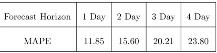
9am, etc. Thus, the temperature forecast accuracy is not simply determined by the forecast horizon (where usually greater forecast horizons correspond to more inaccurate forecasts), but also the volatility of the time period being estimated. Indeed the accuracy (as measured by the mean absolute percentage error) does reduce as a function of horizon, as shown in Table 1, for the full data set. 230
Forecasting temperature four days ahead (i.e. between 73 and 96 hours ahead) has dropped in accuracy by around 100% compared to up to one day ahead (between 1 and 24 hours ahead). For the test set the temperature forecast accuracy is improved compared to the training set (see Table 5 in Section 5.4).
Forecast Horizon 1 Day 2 Day 3 Day 4 Day
MAPE 11.85 15.60 20.21 23.80
Table 1: MAPE for the temperature forecasts for different horizon periods (over the period 31stMarch 2014 to 28thNov 2015).
In our analysis we will focus on the relationship between the load forecasts 235
using forecast temperature inputs (ex-ante forecasts) rather than the historical temperature inputs (ex-post forecasts) [46]. Although the forecast and actual temperature values are very strongly correlated (with a pairwise linear correla-tion coefficient greater than 0.95) we will include results for both ex-ante and ex-post versions. We do this for two reasons. Firstly, much of the literature 240
presents so-called “ex-post” forecasts (i.e. those which use the historical tem-perature inputs) and hence comparisons are possible with other research [46]. Secondly, it provides further evidence concerning the causal link between tem-perature and load at the LV level.
As with high voltage load, there are correlations, usually negative, between 245
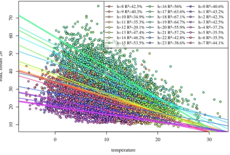
temperature and the LV loads from our feeders. It was found that individual hours of the day typically had, on average, stronger correlations with the tem-perature than the correlations between the complete temtem-perature and load time series. In the Appendix A, we present an example of a feeder from the trial with a relatively strong correlation between load and temperature, showing the 250
linear relationship which varies depending on the hour of the day. This suggests that it may be worthwhile considering splitting the time series into 24 separate, hourly time series for some of our forecasts.
This section has presented some basic analysis of the load data and corre-sponding temperature data. We have highlighted some important features which 255
should be utilised in the load forecasts. Daily, weekly and annual periodicities have strong relationships to load demand and there are different behaviours in demands for different periods of the day. Further, we have seen there is a wide variety of feeders (in terms of numbers of connected customers and magnitudes of demands) with different correlations with the temperature. We will use this 260
information to construct our forecasts as well as appropriate benchmarks.
4. Methods
In this section we present a wide variety of methods which will be used to generate the forecasts. A number of benchmarks are also included for compari-son as well as to highlight the importance of various inputs/predictors.
265
The chosen methods are motivated by the data analysis presented in Sec-tion 3 and are appropriate for volatile data for a number of reasons. First, the kernel density (Section 4.1) and quantile regression (Section4.2) methods have been proven successful in the Global Energy Forecasting Competition (GEF-Com) 2014 [38]. Second, these methods have been successfully applied to more 270
volatile datasets, e.g. the kernel density and the Holt-Winters-Taylor method (Section 4.4) have accurately forecast smart-meter data [40], which are more volatile than LV demand, whereas the autoregressive methods (Section 4.3)
have been applied to volatile financial time-series [47]. Third, the simple sea-sonal regression (Section 4.2) and the autoregressive models have been used to 275
accurately forecast LV demand data for LV feeder storage applications [48]. For these reasons, we believe, that these models are appropriate for volatile data and span a wide range of methods. Further techniques, such as machine learn-ing (e.g. neural networks, support vector machines, etc.) lie beyond the scope of this empirical study and will be the focus of future studies.
280
For this section, without loss of generality, we defineLt,t= 1, ..., N =D·H
to be the hourly time series for the load for a particular feeder, whereH = 24
andD= 612 is the number of days in the training and test data set combined.
The initial time stept= 1 defines the start of the data set 20thMarch 2014 for
the hourly period 12AM to 1AM. Also, without loss of generality, we also define 285
th to denote the end of the historical data (with th+ 1 therefore the start of
the testing period) which determines the maximum available training data for the methods. Specifics of each methods will be described in their corresponding sections.
4.1. Kernel Density Estimation
290
The first method we consider are those based on kernel density estimation (KDE) techniques. These have been successful at generating probabilistic fore-casts for individual smart meter data as well as in the GEFCom 2014 com-petition on higher voltage demand [40, 49]. The method aims to generate a
conditional distribution at time t, f(Lt|X), conditional on historical demand
295
and other factors,X, such as the period of the week or weather variables. The
main challenge of such methods is the computational expense of evaluating the correct parameters, in particular the bandwidths. In this section we presume the
parameters are trained on the historical data [t1, t2], with 1≤t1 < t2 ≤th, t1
modH = 1 andt2 modH = 0, in other words the period of time encapsulates
300
full days from the historical data.
We consider four variations of the KDE methods. The first type, denoted as
hour of the week (1 to 168). The second type, referred to asKDE-Wλ, includes a weighting parameter that favours observations around the same period of the 305
year as the forecasting time, see Appendix B and [49] for further details. Additionally, we consider kernel density estimate forecasts conditioned on
independent variables y, z (CKD), such as the week-period, the temperature,
or both. We produce three CKD forecasts, one conditioned on the week period (CKD-W), a second conditioned on the week period and the actual tempera-310
ture readings (CKD-WTa), and a third forecast conditioned on the both the
week period and the forecast temperature (CKD-WTf). For CKD-W,yi =i
mod 7H is the week period of time interval i. CKD-W weighs observations
to-wards similar times of the week as the forecast time-period. For further details on mathematical formulas, training and parameter optimisation, see Appendix 315
B.
An advantage of the kernel-density methods is that the entire distribution is found simultaneously whereas quantile regression methods only find individual quantiles. The disadvantage is the computational costs, especially as more con-ditional variables are introduced. Various methods, such as clustering the time 320
series, must be employed to reduce the costs [40]. We consider the methods as both probabilistic forecasts and also as point forecasts by using the median of the distributions as our point estimate.
4.2. Simple Seasonal Linear Regression
The method is based on an update of the simple seasonal model presented in 325
[49]. For this method rather than construct a full probability density function for the load distribution we instead develop models for a number of predefined
quaniltesτ∈(0,1). Here, we assume a linear regression model for each quantile,
treating each period of the week as a separate time series of the form
ˆ Lτt = H X k=1 Dk(t) aτk+bτkη(t) + P X p=1 (cτk,p) sin 2πpη(t) 365 + (dτk,p) cos 2πpη(t) 365 ! + 7H X l=1 flτWl(t). (1)
Here, η(k) =Ht+ 1 is the day of the trial (with day 1 as 20thMarch 2014). 330
There are two dummy variables identifying the period of the day, Dk(t), and
the period of the week,Wl(t). Further details of the model can be found in the
Appendix C.
For the point forecast as with the KDE methods we considered the median quantile and also a least squares estimate. In all cases the median outperforms 335
the least squares estimate and hence our point forecast estimates will be derived from the median quantile. The methods are trained on the entire available historical information using the latest data for the rolling forecasts at the start of each new day. Further variants of the model were also considered (different
numbers of seasonal termsP = 2,3, with and without trend (i.e. bk ≡0,∀k),
340
and also using only weekend dummy variables instead of dummy variables for all days of the week), but we found that the best methods used a linear trend,
three seasonal terms (P = 3), and used the day-of-the-week dummy variable as
in equation (1). We also found that the model without trend also performed reasonably well, so in our analysis we will consider both methods. We will 345
denote the seasonal method with trend asSTand without trend asSnT.
Including temperature effects in the model is straightforward and only re-quires adding a polynomial to the full equation (in our case up to only cubic order). Depending on the horizon (one, two, three, or four days ahead) four different models are calibrated.
350
4.3. Autoregressive Methods
The models in this section are all based on a regression of a residual time
seriesrt=Lt−µt, for somemean profileµtwhich we define later. This residual
regression can be written, rk =
pmax X
k=1
φk(rt−k) +t (2)
for some Gaussian error t. The main tunable parameter in the model is
the optimal autoregressive order p=pmax which is chosen by minimising the
φ1, . . . , φmax can then be easily determined by the Burg method. The methods
355
are trained over a year’s worth of historical data prior to the start of the test
period on the 1st October 2015.
For the mean profile µt we consider two models, the details of which can
be found in the Appendix D. The first uses an average weekly profile which we
denote as ARWD. The second updates the simple weekly average profile to
360
include an annual seasonality. We denote this model byARWDY .
As with the ST methods it is trivial to include weather effects by adding linear terms to the mean equations. We note that separate models are used depending on whether the forecasts are one, two, three or four days ahead.
The methods can be updated to generate probabilistic forecast methods by 365
also modelling a variance term using the same features as the mean equation. See Appendix D for further details.
4.4. HWT Exponential Smoothing Method
We implement the Holt-Winters-Taylor (denotedHWT) exponential
smooth-ing method [50] to model the intraday and intraweek seasonality in feeder load. 370
This method is represented as:
Lt = lt−1+dt−s1+wt−s2+φet−1+t et = Lt−(lt−1+dt−s1+wt−s2)
lt = lt−1+λet
dt = dt−s1+δet
wt = wt−s2+ωet, (3)
whereLtdenotes the load observed at timet,ltdenotes the level,t∼IID(0,σ2),
s1= 24,s2 = 168, anddtandwtcorrespond to the intraday and intraweek
sea-sonal indexes, respectively. This model requires the estimation of three
smooth-ing parametersλ,δ andω for the level and two seasonal indexes, along with a
375
parameterφto adjust for first order auto-correlation in the error (denoted by
4.5. Benchmark Methods
As a comparison to the methods presented above, we implemented the fol-lowing four simple benchmarks to model load for each feeder:
380
Benchmark 1, Last Day (LD): Ltˆ +k=Lt+k−s1
Benchmark 2, Last Week (LW): Ltˆ +k=Lt+k−s2
Benchmark 3, Last Year (LY): Lˆt+k=Lt+k−s3
Benchmark 4, Simple Average (SMA): Ltˆ +k= 1p Pp
i=1Lt+k−i×s2
where ˆLt+k is the k-step ahead prediction, t is the forecast origin, whiles1 =
24,s2 = 168,s3 = 52×s2 denote the intraday, intraweek and intrayear cycle
lengths, respectively. For benchmark 4, we considered a variety of different p
values and the best in-sample results were obtained forp= 4,5 weeks, which
385
have very similar scores. We will only present results for p= 5. For further
details regarding these benchmarks methods, please see [51].
4.6. Empirical Estimate
The aforementioned benchmark methods only provide point estimates and hence cannot provide quality comparisons to probabilistic forecasts. For each 390
period of the week we define an empirical distribution function using all the load data from the same time period over the final year of the historical data. We then use this empirical distribution to define the desired quantiles. The median quantile is used as a point estimate. The estimate is fixed over the entire test
period. We refer to this method as the Empirical forecast. Note that we
395
could have included more historical data in the construction of the empirical distribution but by restricting it to the last year we do not introduce seasonal biases.
4.7. Error Measures
To evaluate our methods we consider a variety of forecast measures which 400
the point forecasts we use two common measures, the mean absolute percentage error (MAPE) and the mean absolute error (MAE).
For the probabilistic forecasts we use the continuous ranked probability score (CRPS), which quantifies both the calibration and sharpness of the forecasts
[52]. Suppose we have actual loads a = (a1, a2, . . . , an)T for time periods
ˆ
t1,tˆ2, . . . ,ˆtn and a probabilistic forecast, given by a cumulative distribution
Fk(·) at time ˆtk, then the CRPS is defined by
CRP S(a, F) = 1 n n X k=1 Z ∞ −∞ (Fk(zk)−1(zk−ak))2dzk, (4)
where1is the Heaviside step function. The MAE and CRPS are scale dependent
and therefore we cannot compare feeders of different fundamental sizes. We 405
therefore normalise the score by dividing the MAE and CRPS by the average hourly load of the feeder over the last year of training data. We also multiply the errors by 100 so that they may be referred to as percentages. We refer to these as the relative MAE (RMAE) and relative CRPS (RCRPS) respectively. The CRPS reduces to the MAE in the case of a point forecast and hence we expect 410
them to be strongly related [52]. The MAPE scales each error according to the size of the actual and hence needs no adjustment. The potential disadvantage
of this method is that a few small loads (ak <<1) which are poorly estimated
could skew the average errors.
5. Results
415
In this section we compare the methods we have developed in Section 4. The
test period is the 53 days consisting of 1stOctober 2015 to 22ndNovember 2015
inclusive. Since the temperature forecast data is available from hourly horizons up to 4 days (96 horizons) we will consider up to four day ahead forecasts even when not considering the temperature variables. As described in the Methods 420
section we will construct both point and probabilistic forecasts which will be evaluated using MAPE/RMAE and RCRPS respectively. The test period does not have any holiday dates but does contain a daylight savings change-over on
the 25thOctober 2015. However, this date will not be treated specially in this trial. Special days (public holidays) effects will be considered in future work. 425
5.1. Average Errors
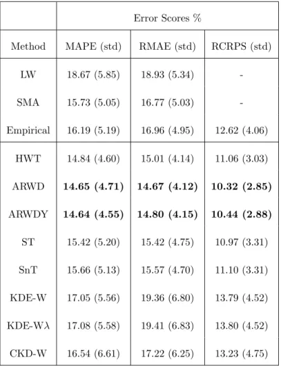
To begin, we consider forecasting techniques without temperature inputs, this will be considered in much more detail in Section 5.4. The average error scores for the methods are shown in Table 2, these consist of the errors for all four day ahead forecasts over the test period. We do not show the LD 430
or LY benchmarks as they are much worse than the Empirical, LW and SMA benchmarks. From comparing the benchmarks we find that the simple average SMA is the best methods for point forecasts and is, in fact, quite competitive with some of the presented methods. In fact it only has an average MAPE of 7% worse than the best methods score, ARWDY. The LY method performs the 435
worst and there is a slight improvement by using the yesterday-as-today estimate LD. The same period of the week forecast, LY, is the best of the random walk methods and shows the strong weekly periodicity of the data.
The most accurate methods for point forecasts are ARWD, ARWDY and HWT which all include daily, weekly and annual periodicities as well as strong 440
autoregressive components. The ARWD and AWRDY methods generate the best forecasts with the ARWD being slightly better in terms of the RMAE. The
HWT is the next best method and has a MAPE of only 1.3% larger than the
ARWD/ARWDY methods. The ST and SnT methods is similar to the AWRDY method but without the autoregressive components and although improves on 445
the benchmarks, only outperforms the SMA by 2%. On average the KDE meth-ods perform the worst only outperforming the random walk methmeth-ods, LD, LW and LY. Conditioning the KDE forecasts on the week period CKD-W improves the forecasts, especially with respect to the RMAE.
For the probabilistic forecasts the empirical benchmark is also shown to be 450
effective and gives a RCRPS only 20% worse than the ARWD method. The ARWD is once again the best forecast, closely followed by ARWDY. This time the ST forecast performs slightly better than the HWT forecast. Of the 100
feeders, the ARWD and ARWDY forecasts were the best performing, with the smallest average errors, for 16 and 26 of the feeders respectively. Hence, there 455
does not appear to be a one-size-fits-all forecast which performs best for all feed-ers and identifying indicators of which forecast to choose will be an important step for practitioners.
Error Scores %
Method MAPE (std) RMAE (std) RCRPS (std)
LW 18.67 (5.85) 18.93 (5.34) -SMA 15.73 (5.05) 16.77 (5.03) -Empirical 16.19 (5.19) 16.96 (4.95) 12.62 (4.06) HWT 14.84 (4.60) 15.01 (4.14) 11.06 (3.03) ARWD 14.65 (4.71) 14.67 (4.12) 10.32 (2.85) ARWDY 14.64 (4.55) 14.80 (4.15) 10.44 (2.88) ST 15.42 (5.20) 15.42 (4.75) 10.97 (3.31) SnT 15.66 (5.13) 15.57 (4.70) 11.10 (3.31) KDE-W 17.05 (5.56) 19.36 (6.80) 13.79 (4.52) KDE-Wλ 17.08 (5.58) 19.41 (6.83) 13.80 (4.52) CKD-W 16.54 (6.61) 17.22 (6.25) 13.23 (4.75)
Table 2: MAPEs, RMAEs and RCRPSs for all forecast methods over all 4 day-ahead forecasts for the entire 53 day test period. The lowest errors for each error score are highlighted in bold. Standard deviations are indicated in the brackets.
5 10 15 20 25 30 Relative MAE (RMAE)
5 10 15 20 25 30 35 Error Error=MAPE Error=RCRPS
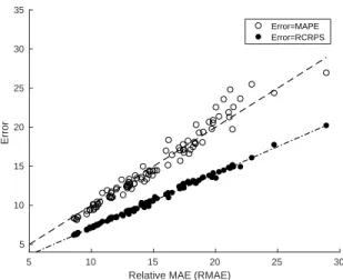
Figure 2: Scatter plot showing the average RCRPS (filled) and average MAPE (unfilled) versus average RMAE for each feeder. Also shown are lines of best fit. These results are for the ARWDY method.
see that the errors are strongly correlated. Figure 2 shows this comparison for 460
the ARWDY method. The plots are very similar for all methods. As expected, the RCRPS and RMAE are strongly related and this corresponds to a very strong linear correlation in the average errors (0.995). The MAPE and RMAE are also strongly correlated (0.981) but with more scatter, especially for larger errors. The strong correlation between the error measures means it is inefficient 465
to present the remaining results in terms of all scores, MAPE, RMAE, and RCRPS. For this reason, and because of the ubiquitous use in the load fore-casting community we will frame the rest of our discussion and analysis with respect to MAPE.
5.2. Forecast Accuracy and Horizon
470
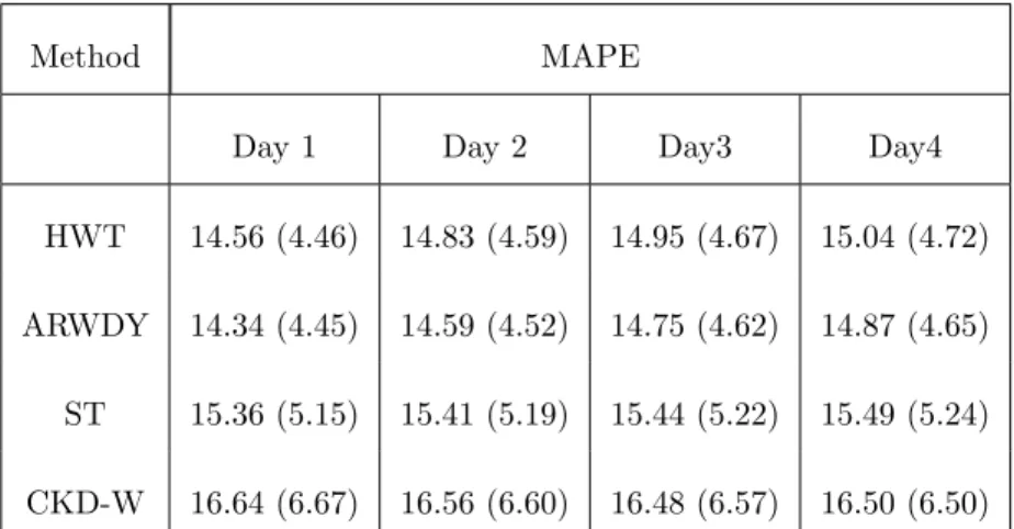
Here we investigate the drop in forecast accuracy as a function of horizon. Initially we consider the forecast accuracy in terms of full days ahead. In other words, we consider the accuracy of forecasts up to 1 day ahead, forecasts between 1 and 2 days, etc. The MAPEs as a function of whole days are shown in Table 3
for selected methods. Specifically, we generate forecasts for horizons at hourly 475
intervals, ranging from one hour up to four days ahead. We use as forecast origin each 7am in the post-sample data, so as to be consistent with the temperature forecast data obtained from the weather station. We note that the benchmarks do not change over the 4 day horizon since they are performed a week in advance. As expected, the most accurate forecasts horizon is one day ahead and the least 480
is 4 days ahead. However, the drop in average accuracy is quite small, with no more than a 4% drop in forecast score.
Method MAPE
Day 1 Day 2 Day3 Day4
HWT 14.56 (4.46) 14.83 (4.59) 14.95 (4.67) 15.04 (4.72)
ARWDY 14.34 (4.45) 14.59 (4.52) 14.75 (4.62) 14.87 (4.65)
ST 15.36 (5.15) 15.41 (5.19) 15.44 (5.22) 15.49 (5.24)
CKD-W 16.64 (6.67) 16.56 (6.60) 16.48 (6.57) 16.50 (6.50)
Table 3: MAPE Scores for each method over each day ahead horizon. Standard deviations are indicated in brackets.
The MAPEs as a function of horizon at the hourly resolution for selected methods are shown in Figure 3a. First recall that the first horizon corresponds
to the period 8−9AM. There are a number of interesting observations. It is
485
clear that all forecast methods produce a similar shape and the more accurate forecasts have smaller errors at all horizons. Secondly, as confirmed with Table 3 there is a general trend with a small overall increase in the error as a function of the horizon. However, the strongest driver of the forecast accuracy is clearly the period of the day. The most inaccurately forecast time periods corresponds to 490
the hours from around 6AM to 6PM. Similarly the period most easily estimated is the evening and night period. Surprisingly, we would expect the evening
0 12 24 36 48 60 72 84 96 12 14 16 18 20 22 24 26
Forecast Horizon (Hours)
MAPE (%) ARWDY LW SMA−5W CKD−W (a) MAPE 0 12 24 36 48 60 72 84 96 6 8 10 12 14 16 18 20 22
Forecast Horizon (Hours)
RCRPS(%)
HWT ST ARWD Empirical
(b) Normalised CRPS Figure 3: Plot of average scores for selected methods for horizons from 1 hour to 96.
period (from 6PM until 11PM) to be quite difficult to forecast. In fact, we discover that the horizon-error shape may be an artifact of the error measure used. In Figure 3b we show the same plot but this time for the relative CRPS 495
score for selected methods. This shows the expected larger error in the evening period. The difference between the two scoring functions is that the MAPE (4) normalises each hourly forecast error with respect to the demand at the same hour. Since for residential feeders (which dominate the composition of the feeders in this trial) have largest demand in this time period the relative 500
error MAPEs are smaller compared to the RCRPS or RMAE. This could have important implications for the use of MAPE in predicting daily errors, especially for the many applications where peak demand is of the most importance, such as in peak demand reduction via storage devices [3]. As evident from Figures 3a and 3b, the forecast errors are high for periods of the day that witness a 505
relatively large change in consumption. We note that since all forecasts start at 7AM each day we have no information on the accuracy of the forecast models as a function of horizon (and regardless of starting point). Encouragingly, the horizon plot shape shown in Figure 3b is consistent with that as shown by the authors in [40] for 800 individual residential customers.
5.3. Accuracy and Feeder Size
As described in the data analysis section the connectivity of the feeders con-sidered varies and consists of different mixtures (domestic and non-domestic) and numbers of customers. Recent literature has shown there is a link between the size of the aggregation which makes up a demand time series and the accu-515
racy of the forecast on a number of different load time series data sets [32, 12]. In contrast to the previous work, these are real networks and hence may have different behaviour compared to aggregations of smart meter data. These net-works include street furniture, such as street-lighting and traffic lights, LCTs, overnight storage heaters, and correlations between neighours are also naturally 520
incorporated.
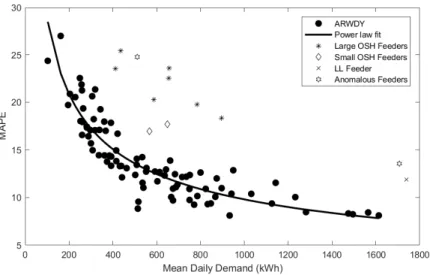
Figure 4: Scatter plot of the relationship between MAPE and mean daily demand for two different forecasting methods. Feeders with unexpectedly large errors have been labeled sep-arately with their known connectivity characteristics (if known). Also shown is a power law fit to the non-anomalous feeders.
Figure 4 shows the MAPEs for each individual feeder as a function of the average daily demand as well. The majority of the feeders appear to fit a power law relationship which fits with the results found in [32, 12]. However, it is clear
that twelve of the feeders do not fit the relationship as tightly as the remaining 525
88 feeders.
After investigation it was found that these particular LV feeders consisted of different connected customers. Firstly, it was found that seven of these feed-ers consisted of unusually large overnight demands most likely due to overnight storage heaters (OSH). In the UK such customers are typically on a special tariff 530
(Economy 7) which provides cheap electricity overnight. Indeed, examination of the connectivity found that 75-85% of customers on each of these seven feeders were on the Economy 7 tariff. These feeders are labelled “Large OSH Feeders” in the figure. Further, two other feeders with smaller overnight demands (but still with noticeable peaks) were discovered and found to have 62% and 75% 535
of their customers on the Economy 7 tariff. These are labelled “Small OSH Feeders” in Figure 4. No other feeders in the 100 were found to have large overnight demands. Finally, the largest feeder of the 100 was also found to have unexpectedly inaccurate forecasts (in relation to the power law fit). This feeder was found to be particularly unusual in that it supplied purely the landlord 540
lighting for an office block. This feeder is labelled “LL Feeder” in the figure. Finally there were two other feeders with anomalous errors (labelled “Anoma-lous Feeders”) but with poor connectivity data and hence we cannot explain the large errors. It is known that one of the feeders has a specific connection for a medical condition which could cause perhaps more irregular demands but this 545
cannot be proven. However, these results do exhibit the important difference between true LV demand and the simple aggregation of smart meter data. In particular, different types of loads and tariffs can have a significant effect on the forecast accuracy.
A power law curve was fitted to the 88 non-OSH/non-anomalous feeders and 550
is included in Figure 4. If the customers producing the aggregated demand were independent and identically distributed (IID) we would expect an exponent of
−0.5, however we found an exponent equal to−0.47 indicating the IID
assump-tion is not completely accurate. Further we found the variaassump-tion of the customers demand also followed a power law curve very similar to the mean errors (not 555
shown).
5.4. Temperature Effect Analysis
Weather, in particular those related to temperature, often plays an impor-tant role in the accuracy of the load forecasts for high voltage level substations [28, 38]. In this section we consider in more detail the impact of including tem-560
perature in the forecasts. In particular, we consider both ex-ante and ex-post forecasts by utilising either forecast or actual temperature values respectively. In reality, ex-ante are the practical way to create true forecasts since, obviously the actual temperature data will not be available ahead of time. However, we include the ex-post forecasts here as well for comparison since much of the lit-565
erature is based on these forms of forecast. Before presenting the analysis, it is important to note that since the temperature forecasts are generated from the fixed time point at 7AM we cannot fully compare the accuracy of the load forecasts as a function of horizon. To do this would require forecasts starting from all time periods of the day.
570
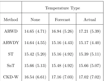
Table 4 shows the MAPEs for the average 4 day ahead forecasts over the test period for selected methods including their updates using temperature data, both actual and forecast values as input. From the table it is clear that the inclu-sion of temperature (either actual or forecast) has minimal effect on the forecast accuracy. In fact for ARWD, ARWDY and CKD-W including the temperature 575
is detrimental to the forecast accuracy. For the ST and SnT methods, there are inconsistent results, using the actual temperature values has little to no effect on the forecast accuracy. Using the temperature forecast values, the
improve-ment on the demand forecast is also very small with at most a 1.7% increase in
forecast accuracy. 580
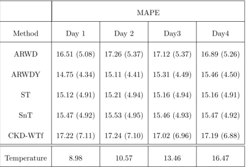
Further, Table 5 shows the accuracy of the ex-ante forecasts as a function of day ahead horizons. Also included is the MAPEs of the temperature forecasts
themselves. The ARWD and ARWDY forecasts drop in accuracy by 5.6% and
4.3% respectively whereas the ST and SnT forecasts hardly change in accuracy
at all. The CKD-W forecast actually improves at the 3-day ahead horizon
Temperature Type
Method None Forecast Actual
ARWD 14.65 (4.71) 16.94 (5.26) 17.21 (5.39)
ARWDY 14.64 (4.55) 15.16 (4.43) 15.17 (4.40)
ST 15.42 (5.20) 15.16 (4.92) 15.39 (5.11)
SnT 15.66 (5.13) 15.48 (4.92) 15.66 (5.07)
CKD-W 16.54 (6.61) 17.16 (7.03) 17.02 (7.02)
Table 4: MAPEs for the methods showing the effect of including temperature data (actual or forecast) for a selection of methods.
compared to the 1-day and 2-day ahead forecasts. These results are in contrast to the accuracy of the temperature forecasts themselves, which drop in accuracy by more than 80% from one day ahead to four days ahead. If the weather was a major driver for the load we would expect a much larger drop in accuracy with horizon. Further, we also considered including up to two lags of the temperature 590
data within the forecast methods but this also had no effect on the accuracy of the forecasts. In particular, we note that the CKD-W method naturally contains lags within the model. Further investigation into the effects of temperature lags is beyond the scope of this research and will considered in a future paper.
Moreover, we investigate the temperature effect in more detail for the AR-595
WDY forecast as a function of feeder size. We only consider day ahead forecasts since this is when the temperature forecasts are most accurate (as shown in Ta-ble 5). To test this relationship, we plotted the difference in MAPE for the ARWDY model (with and without actual temperature) versus feeder size, see Figure E.8 in Appendix E. The plot is similar when using the forecast tem-600
MAPE
Method Day 1 Day 2 Day3 Day4
ARWD 16.51 (5.08) 17.26 (5.37) 17.12 (5.37) 16.89 (5.26) ARWDY 14.75 (4.34) 15.11 (4.41) 15.31 (4.49) 15.46 (4.50) ST 15.12 (4.91) 15.21 (4.94) 15.16 (4.94) 15.16 (4.91) SnT 15.47 (4.92) 15.53 (4.95) 15.46 (4.93) 15.47 (4.92) CKD-WTf 17.22 (7.11) 17.24 (7.10) 17.02 (6.96) 17.19 (6.88) Temperature 8.98 10.57 13.46 16.47
Table 5: MAPE Scores for different day ahead horizons for a selection of methods based on utilising forecast temperature values. Also for comparison is the average MAPE for the temperature forecasts themselves.
found that, irrespective of the feeder size, including temperature (either actual or forecast) as an explanatory variable did not result in an improvement in the out-of-sample forecast accuracy. We observe, from comparing the MAPEs for each feeder, that including the temperature forecasts only improves the errors 605
for 19 of the 100 feeders. If we use the temperature actuals in the forecasts, this only improves a total of 20 feeders forecasts (18 of which are common to the 19 improved feeders using the forecast temperature). In all cases the MAPEs do not improve by any more than 4%.
To further test the effect of including the temperature we also consider com-610
paring the change in the distribution of the MAPEs. We do this by using the two-sample Kolmogorov-Smirnov test (implemented using kstest2 in Matlab) at the 5% significance level. Since we have observed that the different hours of the day have different distributions of demand we split the errors according to both hour (1 to 24) and feeder. This gives us 2400 distributions to compare. Com-615
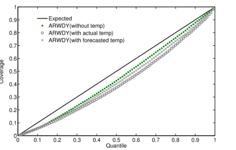
0 0.1 0.2 0.3 0.4 0.5 0.6 0.7 0.8 0.9 1 0 0.1 0.2 0.3 0.4 0.5 0.6 0.7 0.8 0.9 1 Quantile Coverage Expected ARWDY(without temp) ARWDY(with actual temp) ARWDY(with forecasted temp)
Figure 5: Reliability diagram (coverage) for the ARWDY model: (a) without temperature, (b) with actual temperature, and (c) with forecasted temperature. The solid line along the diagonal represents the expect coverage. The coverage values were average across all 100 feeders, and across all 96 horizons.
paring the ARWDY without and with the temperature forecasts as input we find that the null hypothesis (of the errors coming from the same distribution) is only rejected for a total of 79 distributions. Of these, they are split across 36 of the feeders with no more than 5 distributions failing the null hypothesis on any single feeder. Further to this, of the 79 distributions failing the null 620
hypothesis all occur between 11PM and 6AM. In other words, when utilising temperature in the forecasts, all of the significant changes occur during the early morning hours when demand is usually more stable. There is no obvious feeder types for which the overnight errors are larger/smaller than average (and this includes to relationship to the OSH feeders in particular). In addition, when the 625
distributions are significantly changed by including the weather, the accuracy is not improved for any of the forecasts error distributions when compared with not including temperature. Similar results hold when using the actual temper-ature but only 82 distributions are significantly changed (i.e. reject the null hypothesis in the ks-test).
630
a reliability diagram, Figure 5, using the ARWDY model (with and without
temperature). Overall, we found that the inclusion of temperature did not
result in a reduction in modelbias (difference between expected and obtained
coverage) across all quantiles considered in this study, these results are consistent 635
with our findings obtained using the MAPE and CRPS.
As shown in Section 3, for some feeders there is a strong correlation be-tween the load and the temperature. However, when we include the effect in our model the accuracy either changes only slightly or, in the case of ARWD, gets worse. A major difference between the ARWD methods and ARWDY, is 640
the lack of a seasonal term. In fact, we find that demand is much more strongly correlated with seasonality than temperature. If seasonality is a stronger driver of demand, then temperature could result in the detrimental performance in ARWD when included in the model. The strong relationship between demand, temperature and seasonality (represented by a simple sinusoidal curve) is illus-645
trated in Figure A.7 in Appendix A. By treating the temperature as a surrogate for the seasonality the ARWD model may erroneously over-train on data which is not related to the load. Further, although the temperature data comes from within 16KM of the centre of Bracknell, this may not be localised enough for accurate forecasts at the feeder level and these short forecast horizons [53, 54]. 650
The evidence thus suggests that at least in this area of the UK there is not a strong causal link between demand and temperature. Seasonality is a stronger driver of the demand. Interestingly at national level, results have shown that univariate models can outperform weather based models at short forecast horizons [54]. However, we are to be careful to extrapolate this further since 655
this is a relatively small area of the UK and we only consider two months of Winter period. These findings underscore the importance of further research to investigate the relationship between LV feeder load and weather. Moreover, it is worth noting that we only had access to single point weather forecasts. Future studies may employ ensemble weather to accommodate uncertainty during the 660
6. Discussion
Short term load forecasts at the low voltage (LV) level are becoming in-creasingly important as electricity networks prepare for a low carbon future. Network solutions such as storage devices and energy management systems will 665
require accurate forecasts to optimise the headroom and potential cost savings. Although there is a large amount of literature of short term load forecasting techniques there is not much investigation or results for LV level demand. Such demand is much more volatile and challenging than high voltage systems and there is still much to learn about the best methods and inputs for accurate 670
forecasts.
In this paper we have presented several short term forecasting methods, both point and probabilistic, and tested them on 100 real LV feeders. We also compared them to a number of benchmarks, some of which are quite compet-itive. As a consequence of the studies we have found some interesting results. 675
Accurate forecasts can be obtained by relatively simple methods, in particu-lar, a simple average of the previous four weeks performs quite well. The best performing methods were those based on autoregression methods and a Holt-Winters-Taylor exponential smoothing method. However, it was found there was no single method which was the most accurate for a high proportion of 680
feeders.
We also illustrated some important drivers for the accuracy of the forecast. Firstly, the size of the feeder was one of the biggest determining factor for the accuracy, with smaller feeders being more difficult to predict than larger feeders, confirming a known result from the literature. Secondly, the presence of (poten-685
tially high demand) technologies, and specifically overnight storage heaters, had significant implications in the forecast accuracy, modifying the existing power-law relationship between forecast accuracy and aggregation size. This is a novel result and could have important implications for making planning decisions such as making optimal investments in where to install storage. Thirdly, we found 690
more important than the forecast horizon. Errors only increased by 2% from one day ahead to 4% for four day ahead forecasts.
In contrast to HV level load forecasts, temperature was not an important factor in the accuracy of our forecasts. We presented some detailed analysis of 695
the results to show that the temperature either had little or no effect on the forecast accuracy, but in many cases was actually detrimental to the accuracy. We provided one potential explanation which highlighted how the strong corre-lation between load and temperature may in fact be describing a strong seasonal correlation which has more influence on the load than temperature.
700
Finally, we performed some empirical comparison of the forecasts using a variety of error measures. It was found that there was a strong correlation between the scores. Hence, the point-wise scores on the point-wise version of the forecasts could be performed to provide an accurate indication of the accuracy of the corresponding probabilistic forecast. This supports work recently in [44] and 705
could have implications for reducing the cost of model selection for probabilistic load forecasts.
The research presented here can enhance our understanding of the low volt-age network and help network operators make better manvolt-agement and planning decisions for future smart grids. Further the short term load forecasts results 710
lay a foundation for methodologies and metrics to be used for generating and assessing probabilistic LV level load forecasts. In particular, there is still fur-ther understanding into the effects of weafur-ther and LCTs, the role of LV network connectivity and better probabilistic forecasts.
Acknowledgements
715
We would like to acknowledge the support of Scottish and Southern Elec-tricity Networks (SSEN) and its personnel during the collaboration of the New Thames Valley Vision Project (SSET203 New Thames Valley Vision), funded by the Ofgem. We would also like to thank Dr Tamsin Lee for early discussions on the paper.