1
Available online at www.prace-ri.eu
Partnership for Advanced Computing in Europe
Performance Analysis and Enabling of the RayBen Code for the
Intel® MIC Architecture
A. Schnurpfeil
a*, F. Janetzko
a, St. Janetzko
a, K. Thust
a, M. S. Emran
b, J. Schumacher
b aJülich Supercomputing Centre, Institute for Advanced Simulation,Forschungszentrum Jülich, D-52425 Jülich, Germany
bInstitut für Thermo- und Fluiddynamik, Postfach 100565,
Technische Universität Ilmenau, D-98684 Ilmenau, Germany
Abstract
The subject of this project is the analysis and enabling of the RayBen code, which implements a finite difference scheme for the simulation of turbulent Rayleigh-Bénard convection in a closed cylindrical cell, for the Intel® Xeon Phi coprocessor architecture. After a brief introduction to the physical background of the code, the integration of Rayben into the benchmarking environment JuBE is discussed. The structure of the code is analysed through its call graph. The most performance-critical routines were identified. A detailed analysis of the OpenMP parallelization revealed several race conditions which were eliminated. The code was ported to the JUROPA cluster at the Jülich Supercomputing as well as to the EURORA cluster at CINECA. The performance of the code is discussed using the results of pure MPI and hybrid MPI/OpenMP benchmarks. It is shown that RayBen is a memory-intensive application that highly benefits from the MPI parallelization. The offloading mechanism for the Intel® MIC architecture lowers considerably the performance while the use of binaries that run exclusively on the coprocessor show a satisfactory performance and a scalability which is comparable to the CPU.
*
2 1.Introduction
1.1.Scientific Background
Convective turbulence which is driven by the action of the buoyancy force appears in a wide range of geophysical and astrophysical systems as well as in numerous technological applications such as chip cooling devices and indoor ventilation systems. The thermal convection phenomena caused by the vertical temperature gradient is known as the Rayleigh-Bénard convection (RBC). The Rayleigh-Bénard convection model is the widely used one because it can be studied in a controlled manner, but it still has enough complexity to retain the key features of convective turbulence. RBC in cylindrical cells (Figure 1) has been studied intensely over the last decade in several laboratory experiments, mostly in slender cells of aspect ratio smaller than or equal to unity in order to reach the largest possible Rayleigh numbers or to resolve the detailed mechanisms of turbulent heat transport close to the walls [1, 2]. With the advent of powerful supercomputers, direct numerical simulations (DNS) have grown such that the detailed dynamical and statistical aspects of the involved turbulent fields and
their characteristic structures can now be unravelled in detail.
1.2.Equations of motion and numerical model
Three-dimensional Navier-Stokes equations for incompressible fluid in the Boussinesq approximation are solved in combination with the advection-diffusion equation for the temperature field. The system is given by
( ) ( ) (1) (2) (3) where p(x, t) is the pressure, u(x, t) the velocity field and T(x, t) the total temperature field.
The equations are discretized in cylindrical coordinates by a second-order finite difference scheme [3, 4]. The pressure field is determined by a two-dimensional Poisson solver after applying one-dimensional fast Fourier transform (FFT) in the azimuthal direction. The tensor product decomposition method is applied to solve the Poisson equation. The time advancement is done by a third-order Runge-Kutta scheme. The grid spacings are non-equidistant in the radial and axial directions. The DNS grids N1×N2×N3 used satisfy the Grötzbach criterion [5]. The grid resolutions require special attention for calculating the gradient fields [6], in particular for lower Prandtl numbers Pr << 1 the DNS grids must be much finer than the one prescribed by Grötzbach. The code is MPI parallelized (1D-Domain decomposition) in conjunction with OpenMP threading.
PRACE-1IP WP7: Enabling Petascale Applications
3
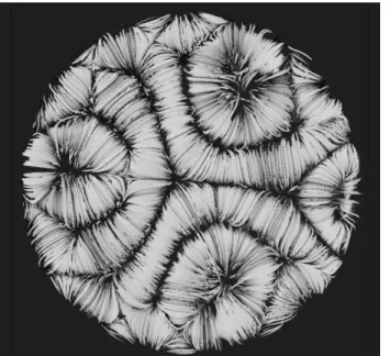
The present code RayBen has been a workhorse for many research activities in Rayleigh-Bénard convection for almost two decades. Thus far we have successfully employed this code to conduct some of our research work listed in [2, 6, 7, 8, 9, 10, 11]. Large scale circulation patterns from one of our simulations are shown in Figure 2.
2.Performance Analysis and Enabling
2.1.Integration of the RayBen Code into the JuBE framework
In order to perform analysis and benchmark runs the RayBen code was integrated into the Jülich Benchmarking Environment JuBE [12]. JuBE provides a script-based framework to easily create benchmark sets, run those sets on different computer systems and evaluate the results. It is written in Perl. Each execution system as well as the different steps of the benchmark runs (compilation of the code, preparation of the input deck, executing the code, verification and finally analysis of the simulation results) are configured using customizable xml-based files. These configuration files need to be adapted only once for each execution system and for each code. The actual parameter space including code specific input parameters as well as general benchmark parameters like number of tasks or nodes to be used for a run is spanned in only one top-level benchmark definition file. Once the code is integrated into JuBE all benchmark or simulation runs can be managed with this single file.
The integration of the RayBen code into JuBE for the JUROPA system, the General Purpose Supercomputer at Jülich Supercomputer Centre, was straightforward, since the JuBE configuration file for the JUROPA architecture was already available. For the EURORA cluster the corresponding configuration file had to be generated. The Intel® compiler together with the Intel® Math Kernel Library (MKL) was used for compiling the code. The code-relevant input parameters (lattice dimensions N1, N2, and N3 as well as the number of iterations) were included in the top-level benchmark file.
The numerical correctness of the benchmark simulations was verified by comparing the calculated Nusselt numbers, which represents the dimensionless heat transfer coefficient, at the bottom and top plate and the Nusselt number averaged over the complete volume with the corresponding reference values. Finally, timing results were taken from the information provided by the code. The wall time and the CPU time for the complete simulation are reported as well as the time needed for each iteration step of the code. Unless noted otherwise all timings discussed in this paper refer to this iteration time.
While the integration of program packages in JuBE on host only systems proved to be straightforward, more attention has to be paid when JuBE is used on architectures equipped with some coprocessors, in particular with Intel® Xeon Phi™ coprocessors. This architecture allows for several combinations to let programs run. Besides the default case where the application only runs on the host CPU, a bunch of other use cases play a role:
Figure 2. Large scale circulation (LSC) patterns at aspect ratio
Γ =12 for Rayleigh number Ra=107 and Prandtl number
4
Host only code, offloading parts of the code on the coprocessor
Natively compiled code running on the coprocessor only
MPI parallelized code running an instant on the host and concurrently on the coprocessor allowing communication between the binaries
Regarding the integration into JuBE all these cases have to be considered which not only affect the execution step but also the compilation of the code. This is not the common use case in JuBE as it usually deals with only one binary at a time. However, JuBE allows any scripting languages in its XML configure scripts such that required functionality can be implemented easily without adapting the JuBE code itself. In fact, all different kinds of binaries were created in one step and packed into a single pseudo binary. The XML configure file for the execution step takes care of unpacking the necessary binaries and automatically creates suitable mpirun/mpiexec options and includes them in a batch script.
2.2.Code Analysis and Debugging
2.2.1.Code Structure of RayBen
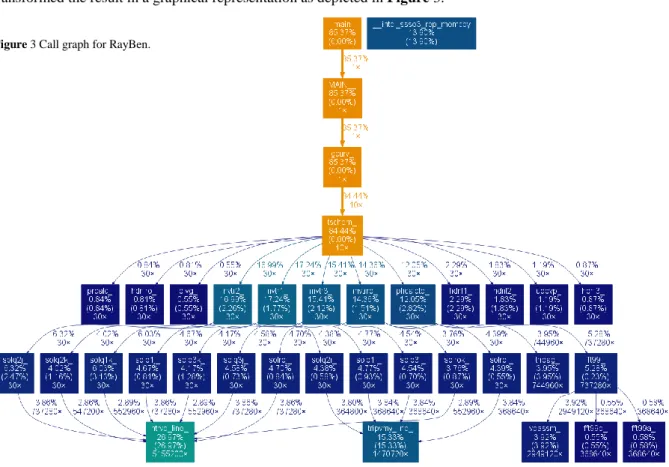
One major question that needs to be answered in this project is whether the RayBen code is suited for the Intel® Xeon Phi architecture using some of the ways this architecture provides to run a code. More precisely, might the code benefit from a native compilation that allows running the code on the coprocessor only and in addition to that might the code benefit from the offload mechanisms provided by this architecture? To get an answer to this question we studied the structure of RayBen and created a call graph. Here, we used gprof and transformed the result in a graphical representation as depicted in Figure 3.
In this figure each routine is represented by a rectangle whereby the colors categorize the amount of time the corresponding routine consumed for the run. Routines colored orange only play a minor role regarding computation time while blue colored routines are more involved ones. The percent values in brackets represent the percentage time the routines consumed in the run, this means the total of this values add to (almost) 100 %. Those percentage values without brackets show the percentage time spent for the routines themselves plus the percentage time for the corresponding children. The third class of values represents how often routines were called by other routines.
PRACE-1IP WP7: Enabling Petascale Applications
5
The call graph shows a layered structure with a one-directional call hierarchy from top to bottom, whereby no calls are carried out between routines of the same layer. The most involved routines occur in the lower part of the graph. Regarding the percentage of time each routine spent in the run it becomes clear, that routines of the lowest level, i.e. ntrvb_line_ and tripvmy_line_ are potential candidates for optimization considerations. At the same time it can be concluded that it might make less sense to implement offload pragmas in those routines as they are called many times from routines of higher layers. In fact this means, each time these routines are called data need to be transferred to the coprocessor resulting in an enormous overhead.
In a second step the OpenMP implementation in RayBen was evaluated with The Intel® Inspector XE 2013 Memory and Thread Analyzer and it has proven that there were some race conditions in the code that were corrected on this occasion. Rechecking the performance of the code showed no significant difference.
2.3.Results on JUROPA
The code was ported and run on JUROPA for comparison. As described in section 2.1 porting of the code to the JUROPA architecture was straightforward using the Intel® compiler suite and MKL. The JUROPA cluster consists of 3288 compute nodes, each equipped with two Intel® Xeon X5570 (Nehalem – EP) quad-core CPUs with 2.93 GHz and 24 GB of RAM (DDR3, 1066 MHz). The nodes are connected by InfiniBand (quad data rate, QDR) with a non-blocking Fat Tree topology.
2.3.1.Benchmark results
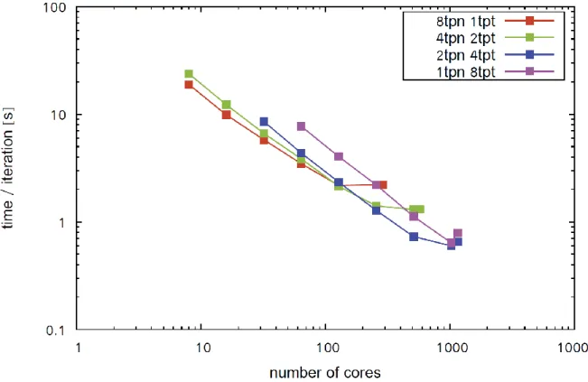
For the benchmark runs on JUROPA a grid size of dimensions N1=433, N2=289, and N3=385 was chosen and the code was run using a pure MPI parallelization as well as different MPI/OpenMP hybrid parallelization setups. Unless noted otherwise the pure MPI setup will be denoted with 8tpn 1tpt (8 tasks per node, 1 thread per task), the hybrid schemes with 4tpn 2tpt, 2tpn 4tpt, and 1tpn 8 tpt, respectively, where tpn means ‘MPI task per node’ and tpt stands for ‘OpenMP thread per MPI task’. For example, 2tpn 4tpt means that on each compute node 2 MPI tasks were started and each of these tasks spawned 4 OpenMP threads.
The benchmark results obtained on JUROPA are given in Table 1 and are depicted in Figure 4.
Table 1: Benchmark results of the RayBen code obtained on JUROPA. Timings data is CPU time in seconds per iteration on average. The compute nodes are used exclusively, i.e. are not shared with other applications.
# cores 8tpn 1tpt 4tpn 2tpt 2tpn 4tpt 1tpn 8tpt 8 18.9 23.0 --- --- 16 9.9 12.3 --- --- 32 5.8 6.7 8.6 --- 64 3.5 3.9 4.4 7.7 128 2.2 2.1 2.3 4.8 256 --- 1.4 1.3 2.2 288 2.2 --- --- --- 512 --- 1.3 0.7 1.1 576 --- 1.3 --- --- 1024 --- --- 0.6 0.6 1152 --- --- 0.7 0.8
Looking at the relative scalability (i.e. the maximum number of cores which gives the best performance for that parallelization scheme) the results show that the code scales independently from the parallelization scheme (pure MPI or hybrid MPI/OpenMP) on up to 128 MPI tasks on JUROPA. For the pure MPI scheme 8tpn 1tpt this corresponds to the usage of 128 cores (with 1 MPI task per core). For the hybrid schemes with 2, 4, and 8 threads per MPI task the scalability limit is reached for 256, 512 and 1024 cores, respectively, which in all three cases corresponds again to the usage of 128 MPI tasks.
The comparison of the absolute CPU time per iteration reveals a minimal execution time of 0.6 seconds per iteration on average for the 1tpn 8tpt scheme with using 1024 cores (128 compute nodes). Empty entries in the table (filled with “---“) are omitted either because the number of cores is too large for the chosen grid size or the timings are irrelevant for testing the scaling behavior of the code.
6
2.4.Results on EURORA
The code has been ported to the Linux Infiniband Cluster EURORA. The EURORA cluster consists of 64 compute nodes, whereof 32 nodes are equipped with 2 Intel® Xeon E5-2658 (Sandybridge) CPUs at 2.10 GHz and the other 32 nodes with 2 Intel® Xeon E5-2687W CPUs at 3.10GHz. 58 nodes have 16 GB of RAM, the other nodes 32 GB RAM per node. Additionally 32 nodes have 2 NVIDIA K20 GPUs each, and 32 nodes are equipped with two Intel® Xeon Phi accelerator card. Each card contains 61 cores with a clock speed of 1.1 GHz each.
Porting the code to the EURORA system was unproblematic. Benchmark runs were performed on the host using two different MPI versions, OpenMPI version 1.6.5 and Intel® MPI version 4.1.2.040. Surprisingly, the scaling behavior of RayBen was very different compared to the behavior on the JUROPA system. Using more than one EURORA node the code profited from increasing the number of cores, however, it showed a much less effective scaling with the Intel® MPI compared with the data obtained on JUROPA. The situation became even worse when OpenMPI was employed. Here the execution time per iteration step increased with the number of cores used. In this case it seems that a disproportional amount of time is spent in MPI routines running on more than one node. The issue is currently further analyzed by members of the CINECA support team. Therefore no scaling results are shown here.
2.5.Results on MIC Systems
The analysis of RayBen regarding the MICs was carried out on the test cluster JUROPA3 at the Jülich Supercomputing Centre. This cluster also includes four Intel® Xeon CPU E5-2650 @ 2.0 GHz nodes with 16 cores whereby each node hosts two Intel® Xeon Phi processors. In principle, two classes of jobs were considered, namely MPI and hybrid runs on the CPU as well as MPI and hybrid runs on the coprocessors. Both classes dealt with two different grid sizes, a small one, as of now referred to as Problem Size 1 with grid dimensions N1=193, N2=97, N3=129 and a big one referred to as Problem Size 2 with grid dimensions N1=433, N2=289, N3=385, i.e. Problem Size 2 is twenty times larger than Problem Size 1.
Figure 4: Scaling behaviour of the RayBen code on JUROPA. The graph shows the average wall time per iteration (seconds) vs. the number of cores used.
PRACE-1IP WP7: Enabling Petascale Applications
7
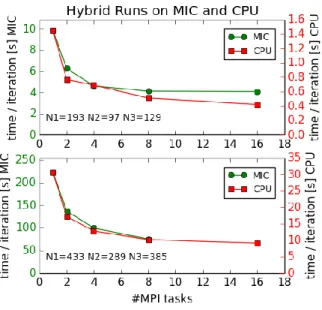
Figure 5 compares hybrid scaling runs on a single node of the MIC and the CPU. The upper panel considers
Problem Size 1 the lower panel Problem Size 2. The needed time per iteration is given in seconds whereby the green colored left axis relates to the run on the MIC while the red colored right axis references CPU runs. In order to ease the comparison of the performance features of both job classes the scales were applied in such a way, that the runs on a single core appear at the same position in the figure.
It is remarkable to notice that both curves in both plots develop in the same way, this means the quality of the performance comply with each other, the simulation times only differ by a constant factor of 7-8 which is due to the different clock speed of the processors and some other hardware characteristics. The MIC run with 16 tasks for Problem Size 2 is missing because of memory limitations.
Moreover, Figure 5 shows the impact of the MPI tasks and OpenMP threads, respectively on the performance of the simulation runs. The number of MPI tasks times the number of OpenMP threads is kept to 16. This means, the number of MPI tasks increases from the left to the right, while the number of involved threads goes down. Figure 5 clearly shows the major role of the MPI tasks, the time per iteration is not constant but lowers the more MPI tasks are involved. This behavior can be observed with
Problem Size 1 and Problem Size 2 as well. Regarding only the MIC runs the performance does not change significantly on four MIC cores and beyond with Problem Size 1 probably due to heavy load on the threads. This behavior can certainly be accounted by the small grid size. In contrast to that the scaling behavior for Problem Size 2 improves, here sufficient workload is spread over the available tasks and threads.
Figure 6 and Figure 7 focus on MPI only on the CPU and the MIC for Problem Size 1 and Problem Size 2. Here, the time per iteration is plotted against the number of cores, which complies with the number of MPI tasks. Again, due to memory limitations on the MICs, the big grid could only be calculated on up to 8 cores. In order to
allow some qualitative comparisons the run time of the MIC runs were scaled to the run time of the CPU in such a way that they meet for the serial run. In fact, this means the iteration time obtained for the CPU is directly shown while the iteration time on the MIC cannot be obtained from the figures. Therefore, the absolute values of the runs are given in Table 2. Of particular note is the concurrency in the qualitative behavior the scaling shows on the CPU compared to the MIC. Furthermore, the scaling itself proved to be decent on both architectures. While this could be expected from the CPU runs in compliance with the results presented in Figure 4, comparable parallel efficiency on the coprocessor is remarkable. The parallel efficiency was calculated according to:
Figure 5 Scaling behaviour of RayBen with different grid sizes. Here the wall time per iteration is plotted against the number of tasks.
Figure 6 RayBen scaling behavior for MPI only, grid size: N1=193, N2=97, N3=129. The exact values are given in Table 2.
Figure 7 RayBen scaling behavior for MPI only, grid size: N1=433, N2=289, N3=385. The exact values can be obtained from Table 2.
8
Where w = wall time per iteration of the serial run, #core = the number of cores in the run and wn is the wall time per iteration of the run on n cores (n = 1, 2, 4, 8, 16, 30, 40, 50, 60).
The efficiency ranges from 0 to 1.0 whereby a value of 1.0 indicates perfect scaling. Figure 6, Figure 7 and Table 2 clearly show satisfying scaling behavior especially for Problem Size 2. Here, the efficiency for the MIC is almost perfect on up to 8 cores while the efficiency obtained for the CPU lowers to roughly 73%. The situation is slightly different for Problem Size 1. Here, the scaling is of lesser quality due to the relatively small grid size, enforcing a lack of work load together with an overhead in communication.
Table 2: RayBen benchmark results for pure MPI runs on the CPU and the MIC coprocessor with different grid sizes. Timing data is wall time in seconds per iteration.
Problem Size 1 Problem Size 2
#cores CPU MIC efficiencyCPU efficiencyMIC CPU MIC efficiencyCPU efficiencyMIC
1 3.88 39.39 1.000 1.000 97.57 926.10 1.000 1.000 2 1.95 19.89 0.995 0.990 48.59 462.14 1.000 1.000 4 1.08 10.40 0.898 0.947 28.30 237.68 0.862 0.974 8 0.69 6.71 0.705 0.734 15.57 115.60 0.783 1.000 16 0.42 4.26 0.579 0.578 9.07 --- 0.662 --- 3.Conclusions
RayBen proved to be a memory intensive application that highly benefits from the MPI parallelization. This outcome plays an important role when it comes to the Intel® Xeon Phi architecture. Here, offloading mechanisms will considerably lower the performance of the code as too much data needs to be transferred too often between the coprocessor and its host. Instead the approach of native binaries, i.e. binaries that run exclusively on the coprocessor becomes an option. Then RayBen shows satisfying performance. However, this behavior is less caused by the threads but mainly by the MPI parallelization. Therefore, it can be concluded, that Intel® Xeon Phi is not the first choice for this kind of code, in particular with regard to the limited memory resources.
References
[1] G. Ahlers, S. Grossmann and D. Lohse, "Heat transfer and large scale dynamics in turbulent Rayleigh-Benard convection," Rev. Mod. Phys., vol. 81, pp. 503-537, 2009.
[2] F. Chilla and J. Schumacher, "New perspectives in turbulent Rayleigh-Benard convection.," Eur. J. Phys. E,
vol. 35, p. 58, 2012.
[3] R. Verzicco and P. Orlandi, "A finite-difference scheme for three-dimensional incompressible flows in cylindrical coordinates.," J. Comp. Phys. , vol. 123, pp. 402-414, 1996.
[4] R. Verzicco and R. Camussi, "Numerical experiments on strongly turbulent thermal convection in a slender cylindrical cell.," J. Fluid Mech., vol. 477, pp. 19-49, 2003.
[5] G. Grötzenbach, "Spatial resolution requirements for direct numerical simulation of the Rayleigh-Benard convection.," J. Comput. Phys., vol. 49, pp. 241-269, 1983.
[6] J. Scheel, M. S. Emran and J. Schumacher, "Resolving the finite-scale structure in turbulent Rayleight-Benard convection.," New J. Phys., vol. 15, p. 32p, 2013.
[7] M. S. Emran and J. Schumacher, "Fine-scale statistics of temperature and its derivatives in convective turbulence.," J. Fluid Mech., vol. 611, pp. 13-34, 2008.
[8] M. S. Emran and J. Schumacher, "Lagrangian tracer dynamics in a closed cylindrical turbulent convection cell.," Phys. Rev. E, vol. 82, p. 016303, 2010.
Rayleigh-PRACE-1IP WP7: Enabling Petascale Applications
9 Benard convection.," Eur. J. Phys. E, vol. 35, p. 108, 2012.
[10] N. Shi, M. S. Emran and J. Schumacher, "Boundary layer structure in turbulent Rayleigh-Benard convection," J. Fluid Mech., vol. 706, pp. 5-33, 2012.
[11] J. Bailon-Cuba, M. S. Emran and J. Schumacher, "Aspect ratio dependence of heat transfer and large-scale flow in turbulent convection.," J. Fluid Mech., vol. 655, pp. 152-173, 2010.
[12] W. Frings, A. Schnurpfeil, S. Meier, F. Janetzko and L. Arnold, "A Flexible, Application and Platform-Independent Environment for Benchmarking.," in Parallel Computing: From Multicores and GPUs to Petascale, Amsterdam, 2010.
Acknowledgements
This work was financially supported by the PRACE-1IP project funded in part by the EUs 7th Framework Programme (FP7/2007-2013) under grant agreement no. RI-261557.