A NEW STRATEGIC CAPACITY PLANNING PROCESS FOR RAILWAY TRANSPORTATION

(1)

2041

中華民國運輸學會98年

學術論文研討會

中華民國 98 年 12 月

A NEW STRATEGIC CAPACITY PLANNING

PROCESS FOR RAILWAY TRANSPORTATION

Yung-Cheng (Rex) Lai1 Mei-Cheng Shih2

ABSTRACT

The demand for railway transportation is expected to be significantly increased worldwide; hence railway agencies are looking for better tools to allocate their capital investments on capacity planning in the best possible way. In this research we developed a capacity planning process to help planners enumerate possible expansion options and determine the optimal network investment plan to meet the future demand. This framework includes an “Alternatives Generator” that generates possible expansion options and an “Investment Selection Model” that determines which portions of the network need to be upgraded with what kind of capacity improvement options. Railway agencies can use this tool to maximize their return from capacity expansion projects and thus be better able to provide reliable service to their customers, and return on shareholder investment.

Keywords: Railway Capacity Planning, Capacity Model, Decision Support

1. INTRODUCTION

The demand on railway transportation in the near future is expected to be significantly increased worldwide (Ministry of Transportation and Communications, 2009; American Association of State Highway and Transportation Officials, 2007). Therefore, the network capacity has to be improved to accommodate this future demand. For example, the Taiwan government is currently upgrading Taiwan Railways Administration (TRA), a conventional mainline railway system, in order to provide high frequency of commuter services in urban areas along the west corridor of Taiwan. The improvement projects include grade separation, building additional commuter stations, adding train sets, and etc. These projects usually require a great amount of capital investment hence railway agencies are looking for better tools to allocate their resources on capacity planning in the best possible way.

1 _{Assistant Professor (Department of Civil Engineering, National Taiwan University,}

yclai@ntu.edu.tw)

2_{Graduate Research Assistant(Department of Civil Engineering, National Taiwan University,}

(2)

2042

Since decades ago computer simulation tools have been developed to help the long-term capacity planning process (HDR, 2003; Canadian National Railway, 2005; Vantuono, 2005); however, the complete process so far still requires human intervention and expert judgments because of the complexity of the problems. Experienced railroaders often identify good solutions, but this does not guarantee that all good alternatives have been evaluated or that the best one has been found. Simulation can model a section of the network in great detail but it is not suitable for network capacity planning (Krueger, 1999). Instead of solving the real problem, solutions based on corridor-based simulation analyses may move bottlenecks to other places in the network.

A good capacity planning process should have the ability to generate and evaluate possible expansion alternatives with an appropriate capacity evaluation model, and suggest an optimal network capacity expansion plan. In this research, we proposed a capacity planning framework for the conventional railway in Taiwan with predominantly passenger traffic. The proposed framework includes two components: [1] an “Alternatives Generator” (AG) module generates capacity expansion options; and [2] an “Investment Selection Model” (ISM) identifies the best capacity expansion plan based on options obtained from AG. Using this capacity evaluation tool and capacity planning framework will help railway agencies maximize their return from capacity expansion projects and thus be better able to provide reliable service to their customers, and return on shareholder investment.

2. THE CAPACITY PLANNING PROCESS

The capacity planning framework developed in this research includes two modules: “Alternatives Generator (AG)” and “Investment Selection Module (ISM)” (FIGURE 2). Based on the section properties, the AG enumerates possible expansion engineering options for each section with the associated costs and capacity increases. The ISM then determines which portions of the network need to be upgraded with what kind of capacity improvement options according to the expansion options, budget, and future demand.

FIGURE 2 Flowchart of the proposed capacity planning process.

A similar capacity planning framework was developed by Lai and Barkan (Lai & Barkan, 2008) to assist North American Freight Railroads on their capacity planning projects. Although they are similar,the key modules in the frameworks are completely different. 90% (if not more) of North American Railroads’ traffic are long and heavy freight trains, and they meet and pass in sidings instead of

(3)

2043

stations. On the contrary, TRA runs mostly passenger trains with double track system; hence, meets between trains are eliminated and passes are mostly accomplished inside stations. These differences reflect in both the capacity evaluation method and expansion options in AG, and also the optimization model framework in ISM. In the following sections, we demonstrate the detail of AG and ISM in this proposed capacity planning framework.

3. ALTERNATIVE GENERATOR (AG)

The AG has to automatically generate possible capacity expansion options with their cost and capacity so it needs a tool to evaluate the current state of each link in the network and then generate expansion alternatives with associated capacity increases and construction costs for each of them. The Institute of Transportation (IOT) in Taiwan has recently developed and completed the “Railway Capacity Manual of Taiwan Railway Administration” (IOT, 2008), “Railway Capacity Manual of Taiwan Railway Administration” which is the best available capacity evaluation tool for TRA so was also selected to be the basis of our AG.

3.1 TRA Capacity Manual

To compute the network capacity, TRA capacity manual first divides the whole network into links and nodes where nodes represent stations and links represent the line segment between two adjacent stations. Most existing railway capacity model treats link and node capacity separately but TRA capacity manual does not; It computes capacity for each “section”, including a link and two adjacent stations; this computation method makes it unique and more practical than separate line capacity from station capacity.

The computation process of the TRA manual can be summarized in twelve steps as follows:

yStep 1: Obtain three sets of parameters for capacity computation process:

Infrastructure properties

Train characteristics

Operating parameters

yStep 2: Grouping trains according to their characteristics in speed,

acceleration, deceleration, length, and stopping pattern.

yStep 3: Determining the travel time of every links for each group of trains.

The travel time is usually decided by the scheduled run time in current timetable.

(4)

2044

yStep 4: Determining the cruising speed by 2/3 real average operating

speed plus 1/3 highest speed of each train group in every sections.

y Step 5: Determining the dwell time at each station for each group of trains

by timetable or the estimation of boarding time.

yStep 6: Calculating the signal headway by using TABLES 1, 2, 3 and

equations (1)~(5). TABLE 1 is the formula for computing signal headway which helps users to identify which equation to be used for particular scenarios. TABLE 2 also shows four basic types of station layout: (I) stations with two exclusive or more tracks for each direction. Only the tracks adjacent to the platform are taken into consideration, (II) stations with one exclusive track for each direction and an additional track shared by two directions without interruption from mainline, (III) stations with layout similar to Type II but with interruption from mainline, and (IV) stations with only one track for each direction.

2 1 , 1 2( ) ( ) ( ) 2 ( ) j y i x s x s A o r di a i o b j i a j i j j v v L s B B s T t t t K a G K b G K b G v v + + − = + − + + + + (1) 2 2 1 , 2 2 ( ) ( ) 2 ( ) j e y s x s A p r b j i a i o a j i j j v s v B B B s T t t K b G K a G K b G v v + + − = − + + + + (2) 2 , 1 2 ( ) ( ) 2 ( ) j y i i x n s x s D o r dj a j i b j i a j i j i j v v v L s B B s T t t t K b G K b G K b G v v v + + − = + − + + + + + (3) 2 , 1 2( ) ( ) ( ) 2 ( ) j y i x n s x s D o r dj a i o b j i a j i j j v v L s B B s T t t t K a G K b G K b G v v + + − = − + + + + + (4) 1 , 2 ( ) i i x n n s D o r a i o i v L s B B T t t K a G v − + + + = + + + (5)

(5)

2045

yStep 7: Calculating the critical signal headway by equations shown in

TABLE 4. Where:

ti : Running time of the preceding train i in the section interested (s)

tj : Running time of the following train j in the section interested (s)

yStep 8: Computing the lost time (the expected value of overtaking time) by

equation(6): j i l t t t = − 2 1 (6) Where: tl : Lost time (s)

yStep 9: Computing the operating margins, by equation (7):

) ( _s _l m T t t =β + (7) Where: tm : Operating margins (s)

β : Factor of operating margins to critical signal headway and lost

time, equal to 0.35 in TRA capacity manual

yStep 10: Determining the minimum signal headway, which is the summation

of critical signal headway (the max number between headway in departure station and headway in arrival station), lost time, and operational margins.

yStep 11: Calculating the average signal headway of different combination of

trains in each section. The ratio of different combination of trains can be decided according to the timetable or by equation (8):

=

∑

⋅ =

∑

⋅ ⋅ =

∑

⋅ ⋅ j i i j i j j i ij j i ij ij ij h n n n n n n h p h h , , 2 2 , 1 (8) Where:

hij: Operation headway between type i and type j train

ni : Number of i type of trains (trains)

nj : Number of j type of trains (trains)

n : Total number of trains (trains)

yStep 12: Using the average signal headways in equation (9) to calculate the

capacity of every section:

h Capacity

(6)

2046

TABLE 1 Formula for Computing the Signal Headways

Type of headway Track Usage at Station for Adjacent Train

Speed condition Computation of

signal headway

Arriving interval Same Track Equation (1)

Arriving interval Differnent Track Equation (2)

Same Track Equation (3)

Same Track Equation (4)

Departure interval Different Track Equation (5)

* Whether ot not the departure train reaches the speed limit before leaving the station

Departure interval 2 2 ( ) i i x n a i o v L s B K a G + + > 2 2 ( ) i i x n a i o v L s B K a G + + ≤

TABLE 2 Average Signal Headways under Different Types of Station Layout Type I II III IV Signal headway Departure Arrival Example of station layout

A s T_, T_s_,_D , , 1 , 2 1 2 3 3 s A s A s A T = T + T 1 , ,A sA s T T = , , 1 , 2 3 1 4 4 s A s A s A T = T + T 2 , ,A sA s T T = , , 1 , 2 1 2 3 3 s D s D s D T = T + T 1 , ,D sD s T T = , , 1 , 2 3 1 4 4 s D s D s D T = T + T 2 , ,D sD s T T =

(7)

2047

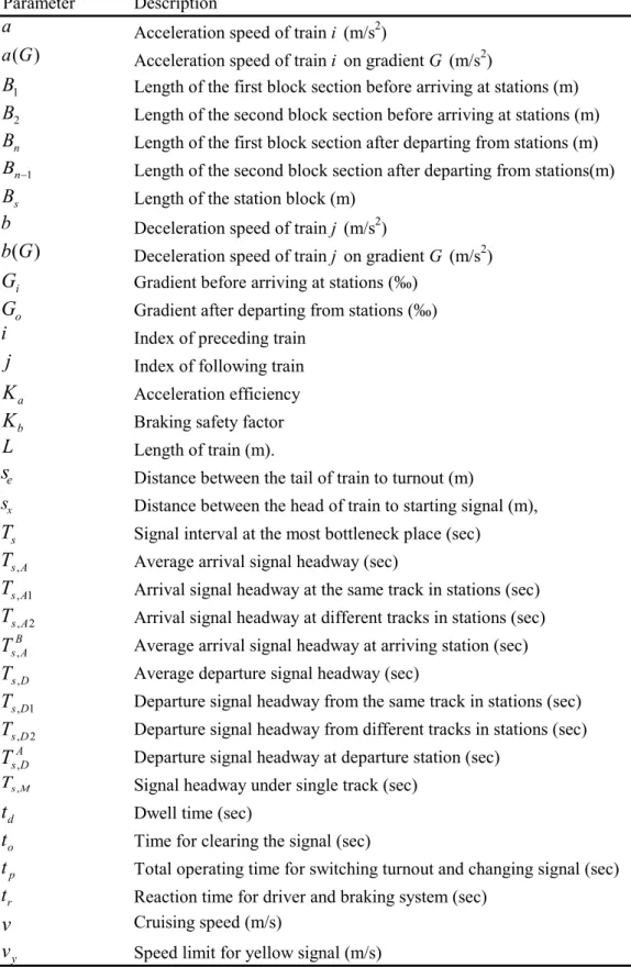
TABLE 3 Notations in TABLE 1 and TABLE Parameter Description

Acceleration speed of train i (m/s2)

Acceleration speed of train i on gradient G (m/s2)

Length of the first block section before arriving at stations (m) Length of the second block section before arriving at stations (m) Length of the first block section after departing from stations (m) Length of the second block section after departing from stations(m) Length of the station block (m)

Deceleration speed of train j (m/s2)

Deceleration speed of train j on gradient G (m/s2) Gradient before arriving at stations (‰)

Gradient after departing from stations (‰) Index of preceding train

Index of following train Acceleration efficiency Braking safety factor Length of train (m).

Distance between the tail of train to turnout (m)

Distance between the head of train to starting signal (m), Signal interval at the most bottleneck place (sec)

Average arrival signal headway (sec)

Arrival signal headway at the same track in stations (sec) Arrival signal headway at different tracks in stations (sec) Average arrival signal headway at arriving station (sec) Average departure signal headway (sec)

Departure signal headway from the same track in stations (sec) Departure signal headway from different tracks in stations (sec) Departure signal headway at departure station (sec)

Signal headway under single track (sec) Dwell time (sec)

Time for clearing the signal (sec)

Total operating time for switching turnout and changing signal (sec) Reaction time for driver and braking system (sec)

Cruising speed (m/s)

Speed limit for yellow signal (m/s) a ) (G a 1 B 2 B n B s B b ) (G b i G o G i j a K b K L e s t s x s s T A s T_, 1 ,A s T 2 ,A s T B A s T_, D s T _, 1 ,D s T 2 ,D s T d t o t p t r t v y v A D s T_, M s T, 1 − n B

(8)

2048

TABLE4 Critical Signal Headway in the Section

Condition Critical block section Critical signal headway

j i t t = j i t t < j i t t > ) , max( _, B_, A s A D s s T T T = )) ( , max( _, B_, _j _i A s A D s s T T t t T = − − ) ), ( max( _, B_, A s j i A D s s T t t T T = − −

The current TRA capacity manual is a good capacity evaluation tool but it does not process capabilities to enumerate possible alternatives and compute the associated construction costs. Therefore, we incorporate expansion enumeration and cost estimation functions into AG (Figure 3).

FIGURE 3 Flowchart of the process in the AG

The purpose of the enumeration function is to automatically generate conventional capacity expansion alternatives for each section in the network based on its current property. Network capacity can be expanded through operational changes or engineering upgrades. Operational options should be considered first because they are usually less expensive and more quickly implemented than building new infrastructure. However, the projected increase in future demand is unlikely to be satisfied by changing operating strategies alone; hence, infrastructure upgrades and expansion are the focus of this research. According to the TRA capacity manual, two most important types of infrastructure-related capacity expansion options are: [1] types of station layout, and [2] effective block length. Therefore, they are incorporated into the alternatives enumeration.

(9)

2049

3.2 Changes in Station Layout and Reduction in Block Length

The layout of a station has the greatest impact on section capacity because it can reduce the signal headways in every links connecting to the station. This effect is prominent especially in the conventional railway system in Taiwan because the congestion usually takes place at the stations. As a result, upgrading the station layout is the most common proposal from the practitioners in order to eliminate bottlenecks. Jong et al. (Jong et al., 2005; Jong et al., 2006; Jong et al., 2009;) has simulated train operations at stations with different types of station layouts. Their study showed that the order of the train headways from small to large is type I, type II, type III, and type IV (TABLE 2). However, according to the TRA capacity manual, type II and type III are different in operating strategies but they are basically the same in terms of infrastructure; therefore, AG treats them the same and computes the associated capacity based on type II station. As a result, in this development there are only three types of station layouts (i.e. type I, type II and type IV).

The shorter the block length, the shorter the spacing between trains and the higher the capacity. Based on the properties of a section, the block length can be reduced to certain predefined levels (i.e. block length) until it reaches the safe braking distance. It is found that the most important blocks to affect section capacity are the “effective blocks” which are those two blocks after departure station (B1 and B2) and two blocks before arriving station (Bn and Bn-1) (FIGURE 4). All the other intermediate blocks have little impact on section capacity and are rarely the bottleneck of the system. Therefore, the effective blocks are the focus of the enumeration process.

B

1

B

2

B

n-1

B

n

Station A

Station B

B

n-1

B

n

B

2

B

1

FIGURE 4 Example of effective blocks.

A link between two stations usually has more than four blocks (i.e. B1, B2, Bn and Bn-1). However, there are links with very short distance where a departure block for a station may also be an arrival block for the next station. In this case, the effective blocks be all blocks between adjacent stations.

3.3 Construction Cost Estimation

The unit construction cost of each type of expansion option is needed to compute the cost of expansion alternatives. Users can specify these values in advance or use the default cost estimates. The default values are based on recent information provided by railroads and engineering consulting companies (TABLE

(10)

2050

5). These values serve as the general average case considering the need for new tracks, signals, and bridges, but do not include the cost of land acquisition or environment permitting.

TABLE 5 Objects in AG and Their Construction Costs Infrastructure Component Cost (USD)

Track 0.549 million/km

Island platform (new build) 1.830 million/platform Side platform (new build) 0.610 million/platform Side platform change into island 0.763 million/platform

Signal 0.100 million/signal

Turnout 0.110 million/turnout

Estimating the cost of reduction in block length is relatively straightforward since tit normally involves additional block signals and changes in track circuit. On the other hand, any change in station layout is complicated. FIGURE 5 is an example of converting Type II station to Type I station. In this case, the Type II station has to go through four processes: [1] adding the additional track for westbound trains (denoted in red lines); [2] adding two signals (one home signal, one starting signal, denoted in green circle), [3] changing the side platform in type II into island platform (denoted in blue words); [4] adding two turnouts (denoted in yellow square) (FIGURE 5).

Island platform Island platform Island platform Island platform : Original tracks : Additional tracks : New turnouts : New signals

: Change in operating strategy

Island platform

Side platform

(11)

2051

3.4 Alternatives Enumeration Process

Each capacity expansion alternative is comprised of “changes in station layout” and/or “reduction in block length”. Below is the procedure of creating all alternatives with their cost and capacity estimation.

yStep 1: Obtain the following input data from existing track condition or users:

Infrastructure properties Train characteristics

Operating parameters

yStep 2: Generating all possible combination between changes in type of

station layout and/or changes in block length. Each combination is regarded as an expansion option and their construction cost were estimated by their infrastructure properties.

yStep 3: Using TRA capacity manual to evaluate the initial capacity and the

capacity of each expansion alternative.

yStep 4:Creating expansion alternatives table.

The final output from AG includes the following information: yDeparture and arrival station of each link

yNew capacity for each engineering options yConstruction cost of reducing block length yConstruction cost of changing station layout

yType of station layout at departure and arriving stations in each option

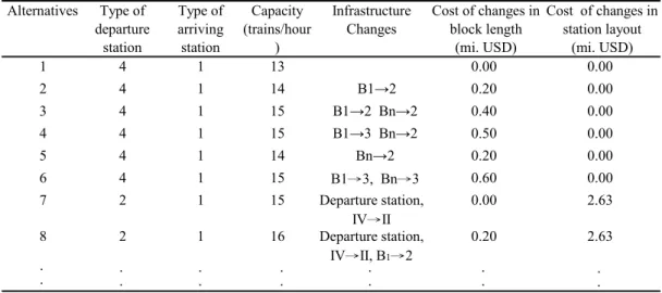
TABLE 6 shows a part of capacity expansion option table in a section which is the final output of AG. For each link, there are usually about 20~30 options but it may get to as much as 100 options. Besides these options, users can also incorporate additional expansion options with the associated costs and capacity into the expansion alternatives table.

(12)

2052

TABLE 6 Expansion Alternatives Table

1 4 1 13 0.00 0.00 2 4 1 14 B1→2 0.20 0.00 3 4 1 15 B1→2 Bn→2 0.40 0.00 4 4 1 15 B1→3 Bn→2 0.50 0.00 5 4 1 14 Bn→2 0.20 0.00 6 4 1 15 B1→3, Bn→3 0.60 0.00 7 2 1 15 Departure station, IV→II 0.00 2.63 8 2 1 16 Departure station, IV→II, B1→2 0.20 2.63 Cost of changes in station layout (mi. USD) Alternatives Type of departure station Type of arriving station Capacity (trains/hour ) Infrastructure Changes Cost of changes in block length (mi. USD) . . . . . . . . . . . . . .

4. INVESTMENT SELECTION MODEL (ISM)

Based on the estimated future demands, budget, and capacity expansion options, the ISM determines an optimal investment plan for capacity expansion. This optimal investment plan identifies sections requiring upgrades and specifies alternatives selected by the ISM. Trains with different origins and destinations can be considered in a manner similar to multiple commodities sharing a common line; therefore, we formulated this problem as a mixed–integer, network design model (Magnanti & Wong 1989;Minoux 1984; Ahuja et al., 1993).

The following notation is used in ISM: o and p are the indexes referring to node as stations and N is the set of all nodes. A is the set of all existing arcs (o, p); δ+(o) stands for the set of the departure station o in certain link and δ-(o) for the arriving station p. K corresponds to the origin-destination (OD) pairs of nodes (s1, t1), (s2, t2), …, (sk, tk) in which sk and tk denote the origin and destination

of the kth OD pair; K represents the set of all OD pairs; q represents the original condition (q=1) and the condition after number (q-1) capacity expansion options is applied (q≥2) and Q is the set of q; m is the type of station layout and M is their set; loq denotes the type of station layout in station o. B is the available

budget; dk is the demand of kthorigin-destination pair; cop stands for the cost of a

unit train passing arc (o, p); hopq indicates the cost of each section associated with

reduction to block length (these changes can be represented by notation q) and

wom indicates the cost of changes m in type of station layout in station r. epk is

the number of trains with O-D pair k requiring to stop at station p. Uop

(13)

2053

capacity expansion option. α and β are the weights to account for the planning horizon.

There are four sets of decision variables in the ISM. The first variable is denoted by xopk which is the number of trains running on arc (o, p) from the kth OD

pair. The second variable goisdenoted for the type of station layout in station o.

The third variable is a binary variable which determining the chosen engineering option q in section (o, p), denoted by yopq. The fourth variable is fom, a binary

variable which determining the final type m of station layout in station o. The following is the optimization model of ISM:

( , ) ( , ) min q q m m k op op o o op op o p A q Q o N m M o p A q Q k K h y w f c x α β ∈ ∈ ∈ ∈ ∈ ∈ ∈ ⎛ ⎞ + + ⎜ ⎟ ⎝

∑ ∑

⎠

∑ ∑∑

(10) s.t. ( , ) q q m m op op o o o p A q Q o N m M h y w f B ∈ ∈ ∈ ∈ + ≤

∑ ∑

(11) =1 ( , ) q op q Q y o p A ∈ ∀ ∈

∑

(12) ( , ) , ( ) q q o op o q Q l y g o p A o δ+ o ∈ = ∀ ∈ ∈

∑

(13) ( , ) , ( ) q q o po o q Q l y g o p A o δ− o ∈ = ∀ ∈ ∈

∑

(14) m o o m M mf g o N ∈ = ∀ ∈

∑

(15) ( ) k k op p o o x e p N δ+ ∈ ≥ ∀ ∈

∑

(16) ( , ) k q q op op op k K q Q x U y o p A ∈ ∈ ≤ ∀ ∈

∑

(17) ( ) ( ) , 0 k k k k po op k k o o o o d if p s x x d if p t p k otherwise δ− δ+ ∈ ∈ ∈ ⎧ ⎪ ⎪⎪ − =⎨ − ∈ ∀ ⎪ ⎪ ⎪⎩

∑

(18)

,

k op o

x

g

∈

{

Integer

},

q , m {0,1} op o y f ∈ (19)

The objective function (equation (10)) aims to minimize the total cost over the planning horizon. This total cost is the summation of costs associated with “changes in block length”, “changes in station layout”, and “transportation cost”. Equation (11) is the budget constraint. Equation (12) ensures each section will select only one capacity expansion option. Equations (13) and (14) maintain the integrity of the station layout since a station can be a departure station or an arrival station for adjacent sections, we have to make sure the type of a particular station is consistent among different decision variables associated with it.

(14)

2054

Equation (15) connects the station layout (go) into notation fom. Equation (16)

ensures trains with kth O-D pair would go through the require stops. Equation (17) is the link capacity restriction ensuring that the total flow on section (o, p) is less than or equal to the capacity under the condition that q expansion option is applied (q = 1) represent for initial state without any expansion option) on arc (o, p). Equation (18) is the network flow conservation constraint guaranteeing that the outflow is always equal to the inflow for trans-shipment nodes; otherwise, the difference between them should be equal to the train of that OD pair.

5. CASE STUDY

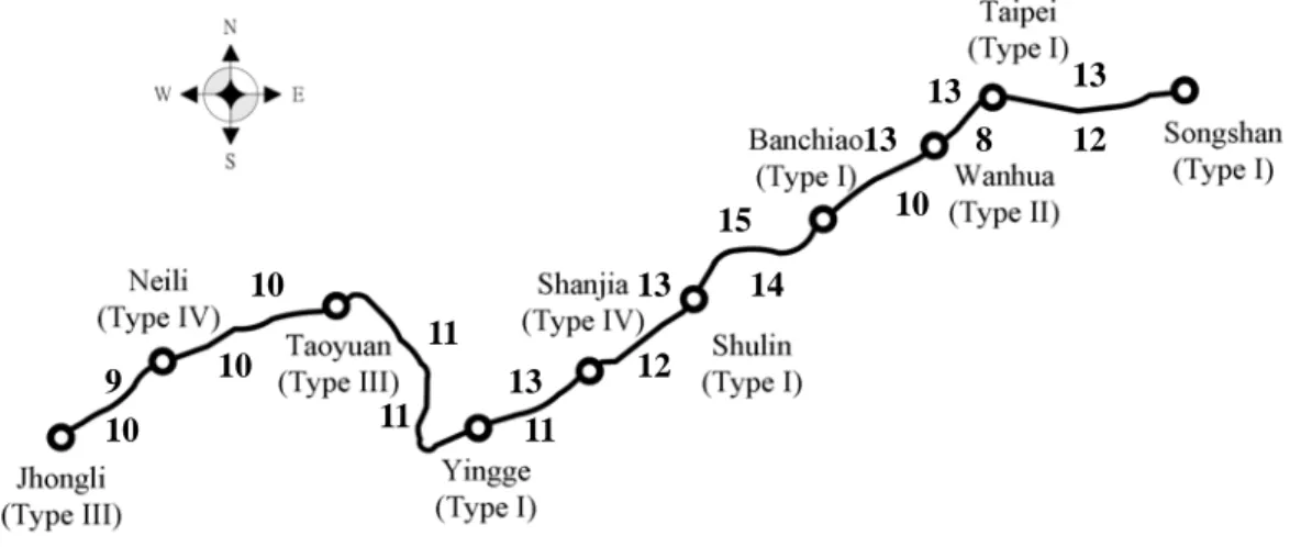
To demonstrate the potential use of the proposed capacity planning process, an actual TRA network from Songshan station to Jhongli station was used in case study (FIGURE 6). The number beside each link is the initial capacity which is evaluated by the TRA capacity manual. In this network, there are total 10 stations and 18 sections (i.e. double track between any two nodes). The current demand is shown in TABLE 7 which is the peak hour demand. This is the busiest part of the TRA network, and has been suffered from deficiency in capacity. Jong et al (Jong et al., 2006) concluded the capacity of some links in this part of network has reached their boundary. This means the network won’t be able to accommodate the demand increase in the future. In this study, we assumed the future demand would increase by 10%, 30% and 50% so the optimal investment plan for each of these scenarios had to be identified.

13 13 13 15 13 13 11 10 9 12 8 10 14 12 11 11 10 10

(15)

2055

TABLE 7 Initial Demands and Final Demands Demand (trains/hr) Demand (trains/hr) 5 5 1 1 5 1 1 2 2 3 2 1 1 O-D pairs Jhongli- Songshan Wanhua- Songshan Shulin- Songshan Jhongli- Taipei Songshan- Shulin Banciao- Jhongli Shanjia- Jhongli O-D pairs Songshan- Jhongli Taipei- Jhongli Songshan- Wanhua Shanjia- Songshan Jhongli- Shulin Songshan- Shulin

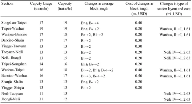
In order to compute capacity by using the AG, we first need to compute the traffic, plant, and operating parameters (Jong et al., 2005). The AG then uses these parameters to enumerate possible capacity expansion options. As mentioned above, two strategies are considered in the AG to increase capacity: [1] reducing block length, and [2] changing the station layout. Based on these options along with demand and budget, the ISM was then used to determine where and how to upgrade the infrastructure. The process was coded in GAMS and efficiently solved by CPLEX within seconds (GAMS Development Corporation, 2008). TABLE 8 shows the optimal investment plans for different scenarios. An arrow in the TABLE 8 represents a change in the division of blocks or types of stations. For example, “B1 & Bn→2＂means dividing both B1 and Bn into two blocks; Wanhua, II→I represents changing the station type of Wanhua from II to I.

For all scenarios, changes in block length are important and effective in capacity planning even though they are sometimes overlooked by the railway practitioners in Taiwan. TABLE 9 summarized the number of infrastructure changes and total cost for each of the three scenarios. It shows the more the increase in demand, the more the required capital for capacity expansion. However, the increase in cost is not proportional to the increase in demand. This demonstrates that the infrastructure improvement should be conducted for scenarios with large increase in demand; otherwise, it may not be justifiable or the problem can be resolved by using operational changes.

(16)

2056

TABLE 8 Optimal Investment Plan for Scenarios (a) 10% Increase (b) 30% Increase (c) 50% Increase in Future Demand

(a)

Section Capcity Usage (trains/hr) Capacity (trains/hr) Changes in average block length Cost of changes in block length (mi. USD) Changes in type of station layout and cost

(mi. USD)

Songshan-Taipei 17 19 B2 &Bn→4 0.40

Taipei-Wanhua 19 19 B2 & Bn→2 0.20 Wanhua, II→I, 1.61

Wanhua-Banciao 17 18 B2→2, B1→2 0.20 Wanhua, II→I, 1.61

Banciao-Shulin 17 17 B1→2 0.30

Yingge-Taoyuan 13 13 B1→2 0.30

Taoyuan-Neili 13 13 B2→2 0.20 Neili, IV→I, 2.63

Neili- Jhongli 13 15 B1→2 0.20 Neili, IV→I, 2.63

Taipei-Songshan 14 16 B2 & Bn→2 0.20

Wanhua-Taipei 16 18 B1→2, B2& Bn-1→2 0.40 Wanhua, II→I, 1.61

Banciao-Wanhua 16 17 B1→3, Bn-1→2 0.50 Wanhua, II→I, 1.61

Shanjia-Shulin 13 13 B2 &Bn→2 0.20

Yingge- Shinjia 13 13 B1→2 0.20

Neili-Taoyuan 11 13 Neili, IV→I, 2.63

Jhongli-Neili 11 12 Neili, IV→I, 2.63

Total cost (including all alternatives, mi. USD) 7.50

(b)

Section Capcity Usage (trains/hr)

Capacity (trains/hr)

Changes in effective blocks Cost of changes in block length

(mi. USD)

Changes in type of station layout and cost

(mi. USD)

Songshan-Taipei 19 19 B2&Bn→4 0.40

Taipei-Wanhua 21 21 B2 & Bn→3 0.30 Wanhua, II→I, 1.61

Wanhua-Banciao 19 19 B2 & Bn-1→3 0.30 Wanhua, II→I, 1.61

Banciao-Shulin 19 21 B1→2, Bn-1→2 0.40

Shanjia-Yingge 12 14 B2→2 0.20

Yingge-Taoyuan 14 15 B1→2, Bn→2 0.40

Taoyuan-Neili 14 14 B2&Bn-1→3 0.30 Neili, IV→I, 2.63

Taipei-Songshan 15 16 B2& Bn→2 0.20

Wanhua-Taipei 17 18 B1→2, B2& Bn-1→2 0.40 Wanhua, II→I, 1.61

Banciao-Wanhua 17 17 B1→3, Bn-1→2 0.50 Wanhua, II→I, 1.61

Shulin-Banciao 15 17 Bn-1→2 0.20

Shanjia-Shulin 14 14 B1& Bn-1→3, B2 &Bn→2 0.50

Yingge- Shinjia 14 14 B1 &Bn→3 0.30

Taoyuan-Yingge 12 13 B2 & Bn→2 0.20

Jhongli-Neili 12 12 Neili, IV→I, 2.63

(17)

2057

(c)

Section Capcity Usage (trains/hr)

Capacity (trains/hr)

Changes in effective blocks Cost of changes in block length

(mi. USD)

Changes in type of station layout and cost

(mi. USD) Songshan-Taipei 21 21 B1→2, B2 &Bn→3 0.50

Taipei-Wanhua 23 23 B1& Bn-1→2, B2 &Bn→3 0.50 Wanhua, II→I, 1.61 Wanhua-Banciao 21 24 B2& Bn-1→4 0.40 Wanhua, II→I, 1.61

Banciao-Shulin 21 21 B1→2, Bn-1→2 0.40

Shulin- Shanjia 16 21 Shanjia, IV→I, 2.59

Shanjia-Yingge 15 18 B2→2 0.20 Shanjia, IV→I, 2.59

Yingge-Taoyuan 15 15 B1→2, Bn→2 0.40

Taoyuan-Neili 15 17 B2 & Bn-1→2, Bn→2 0.40 Neili, IV→I, 2.63

Taipei-Songshan 17 17 Bn→3 0.30

Wanhua-Taipei 19 19 B2& Bn-1→4 0.50 Wanhua, II→I, 1.61

Banciao-Wanhua 19 19 B1→3, Bn→3 0.60 Wanhua, II→I, 1.61

Shulin-Banciao 17 17 Bn-1→2 0.20

Shanjia-Shulin 15 16 B2 &Bn→2 0.20 Shanjia, IV→I, 2.59

Yingge- Shinjia 15 16 B1 &Bn→2 0.20 Shanjia, IV→I, 2.59

Taoyuan-Yingge 13 13 B2 & Bn→2 0.20

Jhongli-Neili 13 15 Bn→3 0.30 Neili, IV→I, 2.63

Total cost (including all alternatives, mi. USD) 12.30

TABLE 9 Comparisons in Number of Changes and Cost from Scenarios with Different Future Demand

Demand Increase Number of Changes in station layout Number of Changes in block length Cost (mi USD) 10% 2 12 7.50 30% 2 15 9.00 50% 3 16 12.30

6. CONCLUSION

Due to the substantial future traffic demand, railway agencies are looking for tools to allocate their capital investments on capacity planning in the best possible way. Therefore, we developed a strategic capacity planning process in this research. The capacity planning framework includes an “Alternatives Generator” that automatically generates possible expansion options and an “Investment Selection Model” that determines which portions of the network need to be upgraded with what kind of capacity improvement options. This tool can help railway agencies with similar operational environment to maximize their

(18)

2058

return from capacity expansion projects and thus be better able to provide reliable service to their customers, and return on shareholder investment.

Acknowledgments

The authors are grateful to the members in the Transportation Division in Sinotech Engineering Consultants, Inc. for their assistance in this research. This project was funded by National Science Council (NSC) of the Republic of China under grant NSC 97-2218-E-002-032.

REFERENCES

Ahuja, R.K., T.L. Magnanti, and J.B. Orlin (1993), Network Flows: Theory,

Algorithms, and Applications. Prentice Hall, Englewood Cliffs, N.J.

American Association of State Highway and Transportation Officials (AASHTO) (2007) Transportation - Invest in Our Future: America's Freight Challenge, AASHTO, Washington, D.C.

Canadian National Railway (CN) (2005), BCNL Long Siding Requirements, CN, Edmonton, AB.

GAMS Development Corporation (2008), GAMS-A User's Guide, GAMS Development Corporation, Washington, D.C., USA.

HDR (2003). I-5 Rail Capacity Study, HDR, Portland, OR.

Institute of Transportation (IOT) (2008), Railway Capacity Manual of Taiwan

Railway Administration, IOT, Taipei, Taiwan.

Jong, J.C., Lee, C.K., Lu, L.S., Chang, S., Chang, E.F., Lin, K.S., and Liou, J.R. (2005), Rail Capacity Research – Rail Capacity Model for TRA System (1), Publication No. IOT-94-8-12-17, Institute of Transportation (IOT), Ministry of Transportation and Communications, Taiwan.

Jong, J.C., Lee, C.K., Lu, L.S., Chang, S., Chang, E.F., Lin, K.S., and Liou, J.R. (2006), Rail Capacity Research – Rail Capacity Model for TRA System (2), Publication No. IOT-95-58-1228, Institute of Transportation (IOT), Ministry of Transportation and Communications, Taiwan.

(19)

2059

Jong, J.C., Lee, C.K., Chang, S., Chang, E.F., Lin, K.S., and Liou, J.R. (2006), Rail Capacity Analysis for Taiwan Railway System – A Case Study of Keeling to Hsinchu Section, Journal of the Chinese Institute of

Transportation, Vol.18 No. 3, pp.233-264.

Jong J. C., Chang, E.F., and Huang, S.S. (2009), A railway capacity for estimating hourly throughputs, Proceedings of the 3rd IAROR Conference, Zurich, Swiss.

Krueger, H. (1999), Parametric Modeling in Rail Capacity Planning, Proceedings

of Winter Simulation Conference, Phoenix, AZ.

Lai, Y.C., and Barkan, C.P.L. A Quantitative Decision Support Framework for Optimal Railway Capacity Planning (2008), Proceedings of 8th World

Congress on Railway Research, Seoul, Korea.

Magnanti, T.L., and Wong, R.T. (1984), Network Design and Transportation Planning: Models and Algorithms, Transportation Science, Vol. 18, No. 1, pp. 1 – 55.

Minoux M. (1989), Network Synthesis and Optimum Network Design Problems: Models, Solution Methods, and Applications, Networks, Vol. 19, pp.313 – 360.

Ministry of Transportation and Communications (MOTC) (2009)., department of statistics, Taiwan. Monthly Statistics of Transportation & Communications.

www.motc.gov.tw/mocwebGIP/wSite/lp?ctNode=160&mp=1. Accessed July 28,.

Vantuono, W.C. (2005), Railway Age “Capacity is where you find it: how BNSF balances infrastructure and operations”. Railway Age, Feb-01.

(20)