Deep convolution neural network for image recognition

an author's

_{http://oatao.univ-toulouse.fr/21329}

https://doi.org/10.1016/j.ecoinf.2018.10.002

Traoré, Boukaye Boubacar and Kamsu-Foguem, Bernard and Tangara, Fana Deep convolution neural network for

image recognition. (2018) Ecological Informatics, 48. 257-268. ISSN 1574-9541

Deep convolution neural network for image recognition

Boukaye Boubacar Traore

_{, Bernard Kamsu-Foguem}

, Fana Tangara

a_{Toulouse University, Toulouse INP-ENIT, Laboratoire Génie de Production, Ecole Nationale d’Ingénieurs de Tarbes 47, Avenue Azereix, BP 1629, F-65016 Tarbes Cedex,}

France

b_{Université des Sciences, des Techniques et des Technologies de Bamako (USTTB), Faculté des Sciences et Techniques Colline de Badalabougou, ancien Lycée Badala, B.P.}

E 28 11 - FST, 223, Bamako, Mali

Keywords:

Deep learning

Convolution neural networks Pathogen images classification Smart microscope

A B S T R A C T

During an epidemic crisis, medical image analysis namely microscopic analyses are made to confirm or not the existence of the epidemic pathogen in suspected cases. Pathogen are all infectious agents such as a virus, bac-terium, protozoa, prion etc. However, there is often a lack of specialists in the handling of microscopes, hence allowing the need to make the microscopic analysis abroad. This results in a considerable loss of time and in the meantime, the epidemic continues to spread. To save time in the analysis of samples, we propose to make the future microscopes more intelligent so that they will be able to indicate by themselves the existence or not of the pathogen of an epidemic in a sample. To have a smart microscope, we propose a methodology based on efficient Convolution Neural Network (CNN) architecture in order to classify epidemic pathogen with five deep learning phases: (1) Training dataset of provided images (2) CNN Training (3) Testing data preparation (4) CNN gen-erated model on testing data and finally (5) Evaluation of images classified. The resulted classification process can be integrated in a mobile computing solution on future microscopes. CNN can improve the accuracy in pathogens diagnosis that are focused on hand-tuned feature extraction implying some human mistakes. For our study, we consider cholera and malaria epidemics for microscopic images classification with a relevant CNN, respectively Vibrio cholerae images andPlasmodium falciparumimages. Image classification is the task of taking an input image and outputting a class or a probability of classes that best describes the image. Interesting results have been obtained from the CNN model generated achieving the classification accuracy of 94%, with 200 Vibrio cholera images and 200Plasmodium falciparumimages for training dataset and 80 images for testing data. Although this document addresses the classification of epidemic pathogen images using a CNN model, the un-derlying principles apply to the other fields of science and technology, because of its performance and its capability to handle more layers than the previous traditional neural networks.

1. Introduction

The recent development of intelligent data analysis methods brings new opportunities and challenges for a wide variety of scientific pro-blems including risk management and image analysis. In previous

works (Traore et al., 2017), we applied data mining techniques on

sa-tellite images for the discovery of risk areas in epidemiology. Tele-epidemiology is the study of the propagation of human or animal dis-eases, transmitted by water, air or vectors that are related to climatic, meteorological and environmental factors, using information and

communication technologies (Marechal et al., 2008; Traore et al.,

2016). The case study concerned the cholera epidemic in Mopti region,

Mali (West Africa). For that, firstly, we focused on supervised

classifi-cation algorithms (Maximum Likelihood) (Abkar et al., 2000) to process

a set of Landsat satellite images from the same area but on different periods. Secondly, a rule-based machine learning method with asso-ciation rules mining were applied for discovering interesting relations between variables. The results generated from the association rules indicate that the level of the Niger River in the wintering periods and some societal factors have an impact on the variation of cholera epi-demic rate in Mopti town. More the river level is high, at 66% rate of

contamination is high (Traore et al., 2017). It has been established the

nature of links between the environment and the epidemic, and to highlight those risky environments when the public awareness of the problem and the prevention policies are absolutely necessary for miti-gation of the propamiti-gation and emergence of the epidemic situations.

In order to outperform our previous results and strengthen the ca-pacity of epidemic crisis management, this paper explores deep learning

Corresponding author.

images recognition to automatically classify epidemic pathogens images through a microscope. We assist today with the gradual re-placement of many applications based on the old classical techniques of machine learning in computer vision by new and emerging ones with

Deep learning (LeCun et al., 2015;Grinblat et al., 2016). In the same

way, in accordance with (Rosado et al., 2016;Tangpukdee et al., 2009)

there is still a need to improve the accuracy in pathogens diagnosis methods that are focused on hand-tuned feature extraction implying some human mistakes. For instance, malaria parasites may be over-looked on a thin blood film while there is a little parasitemia. Deep Convolutional Neural Networks is the standard for image recognition for instance in handwritten digit recognition with a back-propagation

network (LeCun et al., 1990). CNN help to deal with the problems of

data analysis in high-dimensional spaces by providing a class of algo-rithms y to unblock the complex situation and provide interesting

op-portunities thanks to the symmetry property (Mallat, 2016). Deep

Learning for image classification based on neural networks have be-come the new revolution in artificial intelligence and relevant for several domains: the audible or visual signal analysis, facial recognition (Russakovsky et al., 2015), disaster recognition (Liu and Wu, 2016),

voice recognition, computer vision (Karpathy et al., 2014) and

auto-mated language processing (Hinton et al., 2006). Deep learning is a set

of algorithms which aims to model high-level abstractions in data by

using a deep graph with multiple processing layers (Schmidhuber,

2015). Deep Learning has gained popularity over the last decade, due to

its ability to learn data representations in an unsupervised and su-pervised manner and generalize to unseen data samples using hier-archical representations.

Our studies are oriented towards CNN approach of Deep Learning, while much research has been conducted in this field, to our knowledge rare of them have placed a real emphasis on the CNN for the identifi-cation of epidemic pathogens by microscopic analysis. Therefore, when an epidemic occurs, microscopic analyses are made to confirm or not the existence of the epidemic pathogen in suspected cases. However, there is often a lack of specialists in the handling of microscopes, hence the need to make the microscopic analysis abroad with additional costs (Rosado et al., 2016). This results in a considerable loss of time and in the meantime, the epidemic continues to spread. To save time in the analysis of samples, we propose to make the microscopes intelligent so that they are able to indicate by themselves the existence or not of the pathogens of an epidemic in a sample.

The remainder of this paper is organized as follows. Related works

on Deep Convolution Neural Networks are presented inSection 2. Then

in Section 4, we propose our methodology to classify epidemic pa-thogen images and different results are presented at each step and we present also the software used. Finally, we summarize our work and

conclude inSection 5.

2. Related works

Deep learning is the popular area of machine learning which efforts to learn high-level abstractions in data by utilizing hierarchical

architectures. From (LeCun et al., 2015), the success of Deep Learning is

due to the availability of hardware (Central Processing Units (CPUs), Graphics Processing Units (GPUs), and Hard disk, etc.), machine learning algorithms and massive data, for instance, Mixed National Institute of Standards and Technology (MNIST) handwritten digit data

sets and the ImageNet data (Krizhevsky et al., 2012). Deep Learning is

relevant for several domains: hand-written digit classification, the au-dible or visual signal analysis, facial recognition, disaster recognition, voice recognition, computer vision, and automated language processing (Hinton et al., 2006). In agriculture area, Deep convolutional techni-ques are a benefit to prevent damage caused by agricultural pests, this study improves agricultural production and the storage of crops with the accuracy of 98.67% for 10 classes of crop pest images with complex

farmland background (Luo et al., 2017). In the same area, Grinbat and

his colleagues (Grinblat et al., 2016) use Deep convolutional neural

networks (DCNN) for plant identification by classifying three different legume species: white beans, red beans, and soybeans. For

identifica-tion of rice diseases, Lu and his colleagues (Lu et al., 2017) also use

DCNN techniques through image recognition achieving the accuracy of 95.48% with 500 natural images of diseased and healthy rice leaves and stems. In visual recognition, they explore DCNN to classify a hyper-spectral image with an improved accuracy. For remote sensing scene

classification, Nogueira and his colleagues (Nogueira et al., 2017)

ex-plore three possible strategies namely; full training, fine-tuning, and using ConvNets as feature extractors.

Deep Learning is a kind of Neural Network Algorithm taking me-tadata as an input and processes this data through several numbers of layers of the non-linear transformation to compute the output

classifi-cation. But previously, in Traditional Pattern Recognition (Fig. 1), the

process of feature extraction was made by the expert of the area and/or the programmer and, after that the future list is submitted to classical Network Neuron for the classification of input data. Handcrafted Fea-ture Extractor phase is tedious, requires input data knowledge and fi-nally takes a long time. In deep learning, this painful phase is avoided. The essential property of deep learning algorithms is automatic

extraction of features (Fig. 2). This means that this algorithm

auto-matically grasps the relevant features required for the solution of the problem. This reduces the work of the specialist to select features ex-plicitly, as is the case with traditional pattern recognition methods (Fig. 1). This can be used to solve supervised, unsupervised or semi-supervised types of problems. The Deep Learning Neural Network has at least three hidden layers, usually several layers and so it is deep if it has

more than one stage of non-linear feature transformation (LeCun et al.,

2015). Each hidden layer composed of a set of neurons is responsible for

training the unique set of features based on the output of the previous

layer (fig. 2). As the number of hidden layers increases, the complexity

and abstraction of data also increase.

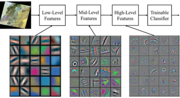
Fig. 3displays the hierarchical model that visualizes the successive phases concerning the features evolution during training process to trainable classifiers. From low-level, mid-level to high-level, each layer's features (set of neurons) are displayed in different components allowing

for Deconvolutional Network approach (Zeiler and Fergus, 2014).

Some researchers divide the deep learning algorithms into four ca-tegories: Convolutional Neural Networks, Restricted Boltzmann

Machines, Auto encoders and Sparse Coding (Guo et al., 2016). In this

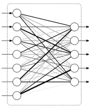
work of images classification, we opted for the Convolutional Neural

Networks (CNNs) (Fig. 4) because they are the widely adapted for

image classification with good performances by making convolutional

networks fast to train (Barbedo, 2013;Krizhevsky et al., 2012).

Convolutional Neural Networks (CNN) approaches are commonly used with architectures having multiple layers that are trained. There

are two stages to train the network: a forward stage and a backward stage. Firstly, the main goal of the forward stage is to represent the input image with the current parameters (weights and bias) in each layer. The first layers find low-level features for instance edges, lines and corners and the other layers find mid-level and high-level features

for instance structures, objects, and shapes (LeCun et al., 2015).

Then the prediction output is used to compute the loss cost to the ground truth labels. Second, based on the loss cost, the backward stage computes the gradient of each parameter with chain rules. All the

Fig. 2.Deep Learning Neural Network.

Fig. 3.Deep Learning: Representations are hierarchical and trained (LeCun et al., 2015).

=

+

u v x u x t v t dt

( )( ) ( ) ( )

(1) The convolution satisfies some algebraic properties (e.g. commu-tativity, associativity, distributivity and multiplicative identity) in order to ensure that the characteristics of their corresponding geometric pictures are preserved.

Commutativity = u v v u (2) Associativity = u (v h) (u v) h (3)

Associativity with scalar multiplication =

a u v( ) (au) v (4)

Distributivity

+ = +

u (v h) (u v) (u h) (5)

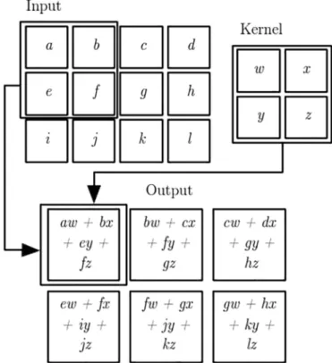
In artificial intelligence, convolutional neural networks apply mul-tiple cascaded convolution kernels with deep learning applications (Fig. 5). Formally, the filtering operation performed by a feature map is a discrete convolution. Discrete convolution can be seen as multi-plication by a matrix. Though, the matrix has several entries with constraints to be equal to other entries.

For functions defined on the set of integers, the convolution of two finite sequences is determined by extending the sequences to finitely applicable functions on the set of integers (e.g. a finite summation may be used for a finite support). The discrete convolution can be defined by

following formula (Hirschman and Widder, 2012):

=

=

u v n u n m v m dt

( )( ) ( ) ( )

m (6)

In image processing, the convolution is done by accomplishing a form of mathematical operation between matrices representing

re-spectively a kernel and an image (Fig. 9). This convolution operation is

made by adding each element of the image to its local neighbors, weighted by the kernel.

The values of a given pixel in the output image are determined by multiplying each kernel value by the matching input image pixel va-lues. This can be represented algorithmically with the pseudo-code il-lustrated below:

Fig. 5.An example of a convolution with Kernel having a 2 × 2 matrix.

parametersareupdatedbasedonthegradientsandarepreparedforthe

next forward computation. After a number of iterations of the forward

andbackwardstages,thenetworklearningcanbestopped.

Clarificationofwhatwasmeantbytheterm“convolution”wouldbe

useful, since it is used to describe mathematical principles and ideas

about the feature transformation approach and process. In

mathe-matics,specificallyin algebraictopology,convolutionis a

mathema-tical transformation on two functions (u and v); it generates a third

function,whichisnormallyviewedasatransformedversionofoneof

theinitialfunctions.Inthecaseoftworealorcomplexfunctions,uand

v the convolution is another function, which is usually denoted u∗v and

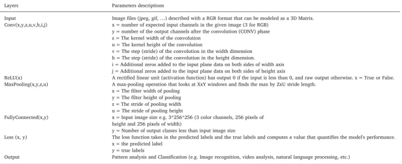
The basic CNN architecture includes Convolution layer, Pooling

layer, ReLU layer and Fully connection layer (as described inTable 1).

Convolution layer

The real power of deep learning, especially for image recognition, comes from convolutional layers. It is the first and the most important layer. In this layer, a CNN uses different filters to convolve the whole image as well as the intermediate feature maps, generating various

feature maps (Fig. 1). Feature map consists of a mapping from input

layers to hidden layers.

We have three hyper parameters to control the size of the output volume of the convolutional layer: the depth, stride, and zero-padding.

•

layer that connect to the same region of the input volume. All of these neurons will learn to activate for different features in the input. For instance, if the first Convolutional Layer takes the raw image as input, then different neurons along the depth dimension may activate in the presence of various oriented edges, or blobs of

color. The depth is 5 in theFig. 6.

Layers Parameters descriptions

Input Image files (jpeg, gif, …) described with a RGB format that can be modeled as a 3D Matrix. Conv(x,y,z,u,v,h,i,j) x = number of expected input channels in the given image (3 for RGB)

y = number of the output channels after the convolution (CONV) phase z = The kernel width of the convolution

u = The kernel height of the convolution

v = The step (stride) of the convolution in the width dimension h = The step (stride) of the convolution in the height dimension.

i = Additional zeros added to the input plane data on both sides of width axis j = Additional zeros added to the input plane data on both sides of height axis

ReLU(x) A rectified linear unit (activation function) has output 0 if the input is less than 0, and raw output otherwise. x = True or False. MaxPooling(x,y,z,u) A max-pooling operation that looks at XxY windows and finds the max by ZxU stride length.

x = The filter width of pooling y = The filter height of pooling z = The stride of pooling width u = The stride of pooling height

FullyConnected(x,y) x = Input image size e.g. 3*256*256 (3 color channels, 256 pixels of height and 256 pixels of width)

y = Number of output classes less than input image size

Loss (x, y) The loss function takes in the predicted labels and the true labels and computes a value that quantifies the model's performance. x = the predicted label

y = true labels

Output Pattern analysis and Classification (e.g. Image recognition, video analysis, natural language processing, etc.)

Fig. 6.Depth process.

Fig. 7.Stride process.

Fig. 8.Zero-padding process.

Fig. 9.Convolution process.

Table1

•

(width and height) are allocated (Fig. 7). When the stride is 1, then

we move the filters one pixel at a time. This leads to heavily over-lapping receptive fields between the columns, and also to large output volumes. When the stride is 2, then the filters jump 2 pixels at a time as we slide them around. The receptive fields will overlap less and the resulting output volume will have smaller dimensions spatially.

•

to pad the input with zeros on the border of the input volume. Zero padding deals with the control of the output volume spatial size. In particular, sometimes it is needed to exactly preserve the spatial size

of the input volume. For example (Fig. 8), the input volume is

32x32x3. If we pad two borders of zeros around the volume, we obtain a 36x36x3 volume. Then, when we apply the convolution layer with our 5x5x3 filters and a stride of 1, then we will also get a 32x32x3 output volume.

There are three main advantages of the convolution operation (Zeiler and Fergus, 2014)

a) the weight sharing mechanism in the same feature map reduces the number of parameters

b) local connectivity learns correlations among neighboring pixels c) invariance to the location of the object.

One interesting approach to handling the convolutional layers is the

Network In Network (NIN) method (Lin et al., 2013), where the main idea

is to substitute the conventional layer with a small multilayer perceptron consisting of multiple fully connected layers with nonlinear activation functions, thereby replacing the linear filters with nonlinear neural net-works. This method achieves good results in image classification. 2.1. ReLU Layer

it is the Rectified Linear Units Layer. This is a layer of neurons that applies the non-saturating non-linearity function or loss function:

=

f (x) max( 0,x) (7)

It yields the nonlinear properties of the decision function and the overall network without affecting the receptive fields of the convolution layer. We have saturated nonlinear functions that are much slower (Krizhevsky et al., 2012). Also, we have the tanh function:

=

f x( ) tanh x( ) (8)

or the logistic sigmoid function: = + f x e ( ) 1 (1 x) ₍₉₎

ReLU results in the neural network that is training several times rapidly, without making a significant difference to generalization ac-curacy.

2.2. Pooling layer

Its task consists to simplify or reduce the spatial dimensions of the information derived from the feature maps. We have three types of pooling: the first one is the average pooling, the second is the L2-norm

pooling and finally the most popular use is the max pooling (Scherer

et al., 2010) because of its speed and improved convergence. This

ba-sically takes a filter (normally of size 2 × 2) (fig. 10) and a stride of the

same length. It then applies it to the input volume and outputs the maximum number in every sub region that has the filter which con-volves around.

2.3. Fully connection layer

The input to this layer is a vector of numbers. Each of the inputs is connected to every one of the outputs hence the term “fully connected”. It is the last layer, in general after the last pooling layer in CNN process (Fig. 11). Fully connected layers perform like a traditional neural net-work and contain about 90% of the parameters in CNN. This layer basically takes as input the output of the last pooling layer and outputs an N dimensional vector where N is the number of classes that the program has to choose from. It allows us to feed forward the neural network into a vector with a predefined length. For image classification, we could feed forward the vector into certain number categories (Krizhevsky et al., 2012). The output is also a vector of numbers. 2.4. Loss layer

Loss layer uses functions that take in the model's output and the target, and it computes a value that measures the model's performance. It can have two main functions:

•

value.

•

associated with the criterion and return the result.

Backpropagation is a principle used to compute the gradient of the loss function (calculates the cost associated with a given state) with respect to the weights in a CNN. The weight updates of

Fig. 10.Max pooling process.

This algorithm uses the training set and performs the above update for each training example. Numerous passes can be made over the training set until the algorithm converges. If this is done, the data can be shuffled for each pass to prevent cycles. Distinctive implementations may use an adaptive learning rate ɛ so that the algorithm converges.

A compromise between computing the true gradient and the gra-dient at a single example is to compute the gragra-dient against more than one training example named a mini-batch at each step. This can achieve meaningfully better than true stochastic gradient descent for the reason that the code can make use of vectorization libraries rather than com-puting each step separately. It may also result in smoother convergence, as the gradient computed at each step uses more training examples.

After this description of the main theoretical elements of neural networks and CNN in deep learning, we will now turn to the application forms in which deep learning activities may be realized. Especially, deep learning can add value by using CNN method to process the images. Concentrating only on health field, the major uses of deep

learning in medical imaging are (Litjens et al., 2017): (i) Classification

(image/exam classification and Object or lesion classification), (ii) Detection (Organ, region and landmark localization, Object or lesion detection) (iii) Segmentation (Organ and substructure segmentation, Lesion segmentation) (iv) registration. In this work, we are focused on epidemic pathogen image classification. Enhancements in accuracy are still needed in pathogens diagnosis methods. Because they are focused on hand-tuned feature extraction, that can imply some mistakes. In addition, the detection of the epidemic pathogen through image

pro-cessing by microscope are relevant in developing countries (Rosado

et al., 2016), this must be considered to make the microscopes more intelligent.

3. METHODOLOGY AND SOFTWARE USED

Diagnosis methods are studied in (Rosado et al., 2016) with the

results from their research works that enhancements in accuracy are still required. For instance, malaria parasites may be overlooked on a

thin blood film while there is a little parasitemia (Tangpukdee et al.,

2009). The objective of this methodology is to classify whether

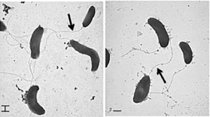
mi-croscopic images are related to either the vibrio cholera (Fig. 12) which

is the responsible of cholera epidemic diseases or to the plasmodium (Fig. 13) for malaria epidemic diseases. We have opted for CNN

ap-proach and TensorFlow open-source software library (TensorFlow,

2018) for machine learning to solve this image recognition problem.

3.1. Methodology to classified epidemic pathogen using CNN

The microscopic analysis consists to confirm or not if the sample is

contaminated by the pathogen Vibrio cholera or by thePlasmodium

falciparum (Harris et al., 2012). Cholera is a contagious epidemic mainly transmitted by infected water containing the pathogen Vibrio

cholera (Davies et al., 2017). Cholera is characterized by sudden and

abundant diarrhoea (gastroenteritis) leading to severe dehydration. In the world, there is a prevalence of 2.8 million cases and the critical victims are close to 100,000 deaths, annually. Vibrio cholera is a gram-negative bacteria, comma-shaped pathogen, mobile and responsible in

Fig. 12.Vibrio cholera (Wang et al., 2017).

Fig. 13.Plasmodium falciparum(Walker et al., 2018)

backpropagationareusuallyperformedthroughthestochasticgradient

descentusingthefollowingalgorithm:

2.5. Algorithmofstochasticgradientdescent

In practice, most practitioners use a procedure called Stochastic

GradientDescent(SGD).Thisconsistsofshowingtheinputvectorfora

few examples, computingtheoutputsandtheerrors, computing the

average gradient for those examples, and adjusting the weights

ac-cordingly. Theprocessisrepeatedforseveralsmall setsof examples

fromthetrainingsetuntiltheaverageoftheobjectivesfunctionsstops

decreasing (LeCun etal., 2015). It is called stochastic because each

small setof examplesgivesanoisyestimate of theaverage gradient

overallexamples.

As illustrated below, it is presented a stochastic gradient descent

algorithmwithaniterativemethod,whichisastochastic

approxima-tion of thegradientdescentoptimization method forminimizing an

humans for cholera, with potential severe consequences as a contagious

epidemic disease (Wang et al., 2017).

Malaria is an infectious disease and remains a leading cause of mortality and morbidity, with an estimated 212 million cases and 429,000 deaths in 2015, worldwide. Malaria is caused by a parasite of

the genusPlasmodium falciparum, spread by the bite of certain species of

Anopheles mosquitoes (Walker et al., 2018).

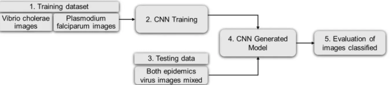
Our methodology consists of five phases as described by the figure

below (fig. 14): (1) Training dataset, (2) CNN for images classification,

(3) Generated model, (4) Testing data and (5) Evaluation of images classified. (1) Provision of training dataset images to the microscope (2) Training of the CNN architecture (3) Preparation of testing data (4) Application of CNN generated model on testing data and (5) Evaluation

of the results provided by the classification before the integration of the solution on future microscopes.

3.1.1. Training dataset

To distinguish cholera pathogen from malaria pathogen images, we need a large image dataset as training dataset. Our training dataset is downloaded from Google images with a keyword about different

epi-demic pathogen names: Vibrio cholera andPlasmodium falciparum, as

shown infig. 15. Training images can be in the most common image

format including jpg, gif, png, tif, bmp etc. They are resized in ac-cordance with CNN classification algorithm format in order to have better results. Training dataset are correctly labeled as a part of the filename, in two categories of images as mentioned above: (i) Vibrio

Fig. 14.CNN for classification of epidemic pathogen.

cholera and (ii)Plasmodium falciparumpathogen images. For our study,

the training dataset contains 400 images of Vibrio cholera and

Plas-modium falciparum.

3.1.2. CNN training

The CNN model is training with seven hidden layers as follow: 6 convolution layers, with the same architecture in each convolution layer followed by a ReLU element-wise nonlinearity and a 2 × 2 MaxPooling. The criterion for choosing of the number of convolution layer is related to the convergence of the error rate during the learning process. In this case, it takes 5 or 6 iterations (particularly by increasing the number of convolution layers) for the calculation to converge. CNN

training architecture for this work is summarized in (Fig. 16).

Sto-chastic gradient descent is used for CNN training using small and equal batches of random data for each iterative learning phase.

3.1.3. Testing data

The testing data is a set of a mixture of an unlabeled Vibrio cholera andPlasmodium falciparumepidemic pathogen (fig. 17). This data is the input of the CNN generated model to predict the label of each image that is the probability that the image is a Vibrio cholera pathogen or Plasmodium falciparumpathogen. For our study, the testing database contains 80 images, named numerically and incrementally.

Fig. 16.CNN Training architecture for this work.

Fig. 17.Some images from our testing data.

3.1.4. CNN generated model

After training step, the CNN generated model is saved in order to load the considered data. The CNNs model is applied at any time with the testing data to evaluate the accuracy of the model. The complete CNN architecture for epidemic pathogen classification adds one fully

connection layer to the Training architecture (fig. 18) and for the final

classifier, we used Softmax function.

3.1.5. Evaluation of classified images

The last step is to evaluate the classified images through the accu-racy and produce the corresponding results. For this study, testing data are the inputs of generated model that is performed to identify images

containing Vibrio cholera or Plasmodium falciparum as output. The

model recognition achieves an improved accuracy of 94% as showing in Table 2and inFig. 19. This figure is calculated from the table generated after apply CNN model.

The software used in this work is the TensorFlow framework (de-scribe below in Section 3.2). TensorBoard is a TensorFlow histograms and graph visualization tool making easy to understand model

para-meters and its variations over time. From thefig. 19, we can note that

this result shows a validation accuracy with 97% and a validation loss with 0.079% allowing to distinguish cholera pathogen from malaria pathogen images. CNN approach can significantly improve the accuracy of pathogens microscopic diagnosis. After CNN classification, the result

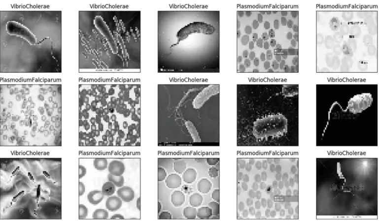
of fifteen random images in testing data are presented inFig. 20.

3.2. Software used: TensorFlow framework

A very flexible deep learning framework, TensorFlow is an open-source software library for Machine Intelligence, developed by Google's researchers and engineers working on the Google Brain Team within

Google's Machine Intelligence research organization (TensorFlow,

2018). It is based on C++ along with python APIs developed, and uses

data flow graphs for performing numerical computations where the nodes represent mathematical operations and the edges represent multidimensional data array communicated between them. TensorFlow supports multiple backends, CPU or GPU on desktop, server or mobile platforms. TensorFlow is highly flexible by running each node on a

different computational device (Bahrampour et al., 2015). For this

study, we deploy TensorFlow on Ubuntu 16.04 through native pip in-stallation, then run our CNN program to produce the above results. 4. DISCUSSIONS

Convolutional neural networks have become a methodology of choice for analyzing medical images analysis especially epidemic pa-thogen images in microscope views. During this work, we note that images of bad qualities impact the classification accuracy. That is why, in the collection phase of image dataset from Google images, we re-moved images not significant, especially those that do not represent microscopic views. This work was achieved manually that could be considered a limitation. In convolution phase, we stopped at six layers because beyond there was no more improvement in the classification accuracy. In summary, we can note that the initial objective was largely achieved to the extent that we were able to obtain interesting results from the CNN model generated achieving the classification accuracy of 94%. These significant results are closely related to good quality image datasets that confirm the importance of data pretreatment.

We must recognize that Deep learning has revolutionized image classification in some fields especially in medical image analyses. Model parameters Training step Accuracy Val_accuracy Loss Val_loss

Values 619 0.9405 0.97 0.23 0.079

620 (last step) 0.9464 0.21

Fig. 19.Different results of classification from Tensorboard.

Table2

However, in the diagnosis of human intestinal parasites, Peixinho and his colleagues proposed an optical microscopy image analysis approach

to discover parasite image features from a small training set (Peixinho

et al., 2015). A relevant review of automatic malaria parasites detection was presented by Rosado and his colleague based on microscopic images segmentation. Image segmentation is the process of portioning

the full image into several subparts (Rosado et al., 2016). In the same

way, Quinn and his colleagues evaluate the performance of deep

con-volutional neural networks on some different microscopy tasks (Quinn

et al., 2016). Their CNN architecture consists only of two convolution layers and also, it's training on segmented images. This preprocessing has an impact on image quality that can be a limitation related to the classification accuracy. The proposed methodology can classify several types of image datasets containing certain characteristics of epidemio-logical pathogens. The practical aspects of its incorporation into the mobile technologies and dedicated solutions like digital microscopes are particularly relevant for developing countries. This helps to (1) fill the lack of microscope (2) cope with the lack of skilled technicians in microscopic manipulation (3) and also facilitate microscopic analysis for accurate diagnosis and thus contributes to an appropriate medical

care for several victims during epidemic crises (Traore et al., 2018).

5. CONCLUSION ANDPERSPECTIVES

In this paper, we presented an approach based on Deep Convolution Neural Network for image recognition. This approach was applied to classify whether microscopic images contain either a cholera or a

ma-laria pathogen, scientifically named Vibrio cholerae and Plasmodium

falciparum. The proposed CNN architecture supplies best classification results achieving the classification accuracy of 94%, with 200 Vibrio

cholera images and 200 Plasmodium falciparum images for training

dataset and 80 images for testing data. The main contributions of this work are the following. Firstly, a support for the decision-making process, because it helps to improve the management of an epidemic

crises by saving time and cost in microscopic analyses. Secondly, in-tegrating this solution into future microscopes helps to have intelligent microscopes. Finally, the smart microscopes can help to fill the gap of specialists in microscopic manipulations and also the lack of technical facilities.

In future works, we intend to explore the well optimized archi-tecture because this one is not clear at all in the literature. For instance, it will be interesting to be able to determine the number of hidden layers and their chronological order, to increasing the effectiveness of the used algorithms. The different architectures are defined by context from one study to another and so it is a challenge to define general architecture from one domain to another in terms of parameters of each layer. There is another challenge to obtain large-scale datasets than

ImageNet (Russakovsky et al., 2015) which contains around

14,000,000 images organized in hierarchical nodes, and the MNIST

database (LeCun et al., 2010) which contains handwritten digit images

composed by 60,000 training images and 10,000 tests images. The ef-ficiency of a CNN model depends on large-scale datasets. We also expect to explore in depth best comprehensive mathematical descriptions, because deep learning architecture hides complex problems and some underlying aspects are still poorly understood in mathematics. Knowing that El Hatri and his colleagues proposed the use of fuzzy logic and back-propagation algorithm to precisely adjust and control the

para-meters in the deep network (El Hatri and Boumhidi, 2017).

ACKNOWLEDGEMENTS

This work is supported by a funding within the grant of “Programme de Formation des Formateurs des Universités de Bamako et de Ségou”, delivered by the Malian government. We want to thank the Doctoral School Aeronautics and Astronautics of Toulouse University whose activities have stimulated the research works described in the content of the paper. We congratulate Shester GUEUWOU for his linguistic ability of proofreading as a native English speaker.

DISCLOSURE STATEMENT

No potential conflict of interest was reported by the authors FUNDING

This work was supported by the “Programme de Formation des Formateurs des Universités de Bamako en république du MALI” with by the CONVENTION DE SOUTIEN A LA FORMATION N°17 - 006 -/ USJPB-R/PFF-A.

REFERENCES

Abkar, A.-A., Sharifi, M.A., Mulder, N.J., 2000. Likelihood-based image segmentation and classification: a framework for the integration of expert knowledge in image classi-fication procedures. Int. J. Appl. Earth Obs. Geoinformation 2, 104–119.

Bahrampour, S., Ramakrishnan, N., Schott, L., Shah, M., 2015. Comparative study of deep learning software frameworks. ArXiv Prepr. In: ArXiv151106435.

Barbedo, J.G.A., 2013. Digital image processing techniques for detecting. quantifying and classifying plant diseases. SpringerPlus 2, 660.

Davies, H.G., Bowman, C., Luby, S.P., 2017. Cholera – management and prevention. J. Infect., Hot Topics in Infection and Immunity in Children 74 (17), 30194–30199.

https://doi.org/10.1016/S0163-4453.S66–S73.

El Hatri, C., Boumhidi, J., 2017. Fuzzy deep learning based urban traffic incident de-tection. Cogn. Syst. Res.https://doi.org/10.1016/j.cogsys.2017.12.002.

Grinblat, G.L., Uzal, L.C., Larese, M.G., Granitto, P.M., 2016. Deep learning for plant identification using vein morphological patterns. Comput. Electron. Agric. 127, 418–424.

Guo, Y., Liu, Y., Oerlemans, A., Lao, S., Wu, S., Lew, M.S., 2016. Deep learning for visual understanding: A review. Neurocomputing 187, 27–48.

Hinton, G.E., Osindero, S., Teh, Y.-W., 2006. A fast learning algorithm for deep belief nets. Neural Comput. 18, 1527–1554.

Hirschman, I.I., Widder, D.V., 2012. The Convolution Transform. Courier Corporation. TensorFlow, 2018. TensorFlow [WWW Document]. TensorFlow. https://www.

tensorflow.org(last accessed on 12 October 2018).

Karpathy, A., Toderici, G., Shetty, S., Leung, T., Sukthankar, R., Fei-Fei, L., 2014. Large-scale Video Classification with Convolutional Neural Networks. In: Presented at the Proceedings of the IEEE Conference on Computer Vision and Pattern Recognition, pp. 1725–1732.

Krizhevsky, A., Sutskever, I., Hinton, G.E., 2012. ImageNet Classification with Deep Convolutional Neural Networks. In: Pereira, F., Burges, C.J.C., Bottou, L., Weinberger, K.Q. (Eds.), Advances in Neural Information Processing Systems 25. Curran Associates, Inc, pp. 1097–1105.

LeCun, Y., Boser, B.E., Denker, J.S., Henderson, D., Howard, R.E., Hubbard, W.E., Jackel, L.D., 1990. Handwritten digit recognition with a back-propagation network. Advances in Neural Information Processing Systems. 396–404.

LeCun, Y., Cortes, C., Burges, C.J., 2010. MNIST handwritten digit database. ATT Labs Online Available Httpyann Lecun Comexdbmnist 2.

LeCun, Y., Bengio, Y., Hinton, G., 2015. Deep learning. Nature 521, 436–444.

Lin, M., Chen, Q., Yan, S., 2013. Network in network. ArXiv Prepr. In: ArXiv13124400. Litjens, G., Kooi, T., Bejnordi, B.E., Setio, A.A.A., Ciompi, F., Ghafoorian, M., van der

Laak, J.A.W.M., van Ginneken, B., Sánchez, C.I., 2017. A survey on deep learning in medical image analysis. Med. Image Anal. 42, 60–88.https://doi.org/10.1016/j.

media.2017.07.005.

Liu, Y., Wu, L., 2016. Geological Disaster Recognition on Optical Remote Sensing Images Using Deep Learning. Procedia Comput. Sci. 91, 566–575.

Lu, Y., Yi, S., Zeng, N., Liu, Y., Zhang, Y., 2017. Identification of rice diseases using deep convolutional neural networks. Neurocomputing 267, 378–384.https://doi.org/10. 1016/j.neucom.2017.06.023.

Luo, X., Shen, R., Hu, J., Deng, J., Hu, L., Guan, Q., 2017. A Deep Convolution Neural Network Model for Vehicle Recognition and Face Recognition. Procedia Comput. Sci. 107, 715–720.

Mallat, S., 2016. Understanding deep convolutional networks. Phil. Trans. R. Soc. A 374, 20150203.https://doi.org/10.1098/rsta.2015.0203.

Marechal, F., Ribeiro, N., Lafaye, M., Güell, A., 2008. Satellite imaging and vector-borne diseases: the approach of the French National Space Agency (CNES). Geospatial Health 3, 1–5.

Nogueira, K., Penatti, O.A.B., dos Santos, J.A., 2017. Towards better exploiting con-volutional neural networks for remote sensing scene classification. Pattern Recognit. 61, 539–556.https://doi.org/10.1016/j.patcog.2016.07.001.

Peixinho, A.Z., Martins, S.B., Vargas, J.E., Falcao, A.X., Gomes, J.F., Suzuki, C.T.N., 2015. Diagnosis of human intestinal parasites by deep learning. In: Computational Vision and Medical Image Processing V: Proceedings of the 5th Eccomas Thematic Conference on Computational Vision and Medical Image Processing (VipIMAGE). 2015. Tenerife, Spain, pp. 107.

Quinn, J.A., Nakasi, R., Mugagga, P.K., Byanyima, P., Lubega, W., Andama, A., 2016. Deep convolutional neural networks for microscopy-based point of care diagnostics. In: Machine Learning for Healthcare Conference, pp. 271–281.

Rosado, L., Correia da Costa, J.M., Elias, D., S Cardoso, J., 2016. A Review of Automatic Malaria Parasites Detection and Segmentation in Microscopic Images. Anti-Infect. Agents 14, 11–22.

Russakovsky, O., Deng, J., Su, H., Krause, J., Satheesh, S., Ma, S., Huang, Z., Karpathy, A., Khosla, A., Bernstein, M., 2015. Imagenet large scale visual recognition challenge. Int. J. Comput. Vis. 115, 211–252.

Scherer, D., Müller, A., Behnke, S., 2010. Evaluation of pooling operations in convolu-tional architectures for object recognition. In: Artificial Neural Networks – ICANN 2010, Lecture Notes in Computer Science. Presented at the International Conference on Artificial Neural Networks. Springer, Berlin, Heidelberg, pp. 92–101.https://doi. org/10.1007/978-3-642-15825-4_10.

Schmidhuber, J., 2015. Deep learning in neural networks: An overview. Neural Netw. 61, 85–117.

Tangpukdee, N., Duangdee, C., Wilairatana, P., Krudsood, S., 2009. Malaria diagnosis: a brief review. Korean J. Parasitol. 47, 93.

Traore, B.B., Kamsu-Foguem, B., Tangara, F., 2016. Integrating MDA and SOA for im-proving telemedicine services. Telemat. Inform. 33, 733–741.https://doi.org/10. 1016/j.tele.2015.11.009.

Traore, B.B., Kamsu-Foguem, B., Tangara, F., 2017. Data mining techniques on satellite images for discovery of risk areas. Expert Syst. Appl. 72, 443–456.https://doi.org/ 10.1016/j.eswa.2016.10.010.

Traore, B.B., Kamsu-Foguem, B., Tangara, F., Tiako, P., 2018. Software services for supporting remote crisis management. Sustain. Cities Soc. 39, 814–927 (May). Walker, N.F., Nadjm, B., Whitty, C.J.M., 2018. Malaria. Medicine (Baltimore) 46, 52–58.

https://doi.org/10.1016/j.mpmed.2017.10.012.

Wang, H., Silva, A.J., Benitez, J.A., 2017. 3-Amino 1,8-naphthalimide, a structural analog of the anti-cholera drug virstatin inhibits chemically-biased swimming and swarming motility in vibrios. Microbes Infect. 19, 370–375.https://doi.org/10.1016/j.micinf. 2017.03.003.

Zeiler, M.D., Fergus, R., 2014. Visualizing and understanding convolutional networks. In: European Conference on Computer Vision. Springer, pp. 818–833.