University of Pennsylvania
ScholarlyCommons
Statistics Papers Wharton Faculty Research
2010
Bayesian Variable Selection in Structured
High-Dimensional Covariate Spaces With Applications
in Genomics
Fan Li
Nancy R. Zhang
University of Pennsylvania
Follow this and additional works at:http://repository.upenn.edu/statistics_papers
Part of theStatistics and Probability Commons
At the time of publication, author Nancy R. Zhang was affiliated with Stanford University. Currently, she is a faculty member at the Statistics Department at the University of Pennsylvania.
This paper is posted at ScholarlyCommons.http://repository.upenn.edu/statistics_papers/512
For more information, please [email protected].
Recommended Citation
Li, F., & Zhang, N. R. (2010). Bayesian Variable Selection in Structured High-Dimensional Covariate Spaces With Applications in Genomics.Journal of the American Statistical Association, 105(491), 1202-1214.http://dx.doi.org/10.1198/jasa.2010.tm08177
Bayesian Variable Selection in Structured High-Dimensional Covariate
Spaces With Applications in Genomics
Abstract
We consider the problem of variable selection in regression modeling in high-dimensional spaces where there is known structure among the covariates. This is an unconventional variable selection problem for two reasons: (1) The dimension of the covariate space is comparable, and often much larger, than the number of subjects in the study, and (2) the covariate space is highly structured, and in some cases it is desirable to incorporate this structural information in to the model building process.
We approach this problem through the Bayesian variable selection framework, where we assume that the covariates lie on an undirected graph and formulate an Ising prior on the model space for incorporating structural information. Certain computational and statistical problems arise that are unique to such high-dimensional, structured settings, the most interesting being the phenomenon of phase transitions. We propose theoretical and computational schemes to mitigate these problems. We illustrate our methods on two different graph structures: the linear chain and the regular graph of degreek. Finally, we use our methods to study a specific application in genomics: the modeling of transcription factor binding sites in DNA sequences.
Keywords
Ising model, Markov chain Monte Carlo, motif analysis, phase transition, undirected graph
Disciplines
Statistics and Probability
Comments
At the time of publication, author Nancy R. Zhang was affiliated with Stanford University. Currently, she is a faculty member at the Statistics Department at the University of Pennsylvania.
Bayesian Variable Selection in Structured High-Dimensional
Covariate Spaces with Applications in Genomics
Fan Li
Department of Health Care Policy Harvard Medical School Boston, MA 02115-2899, USA [email protected] Nancy R. Zhang Department of Statistics Stanford University Stanford, CA 94305-4065, USA [email protected] November 18, 2007 SUMMARY
We consider the problem of regression modeling in high dimensional spaces
where there is known structure among the covariates. Such problems are
be-coming increasingly relevant as high-throughput data collection schemes become increasingly common. A fundamental goal in such problems is to find a small set of covariates that are associated with a response variable, which we discuss from the perspective of statistical variable selection. However, this is an unconventional variable selection problem for two reasons: (1) The dimension of the covariate space is comparable, and often much larger, than the number of subjects in the study, and (2) the covariate space is highly structured, and in many cases it is desirable to incorporate this structural information in the model building process. We approach this problem through the Bayesian variable selection framework, where we formulate a general Ising prior on the model space for incorporating structural information. However, certain computational and statistical problems arise that are unique to such high dimensional, structured settings, the most in-teresting being the phenomenon of phase transitions. We propose theoretical and computational schemes to mitigate these problems. As examples we discuss two specific applications in genomics, one arising from DNA copy number analysis, and the other arising from the modeling of transcription factor binding sites in DNA sequences.
Key words and phrases: Bayesian variable selection, DNA copy number data, Ising model, Markov chain Monte Carlo, motif analysis, phase transition
1
Introduction
Consider the standard multiple regression problem
Y =Xβ+, (1.1)
where Y is n×1 variable response, X = (X1, . . . ,Xm) is a n×m matrix of covariates, and
is an n×1 error term. We employ the standard assumption that ∼ N(0, σ2I). In this paper, we study the problem of variable selection for this model when m is large, possibly much larger than n, and when there is known structure among the covariates which can help us in the model building process.
This scenario of variable selection in a high dimensional structured covariate space appears often in modern applied statistics. In Section 3, we will discuss in detail two problems of this kind that arise in high-throughput genomics. The first problem concerns the analysis of array-based comparative genomic hybridization (array-CGH) data, where the covariates are measurements of DNA quantity atmlocations in the genome, collected fornpatients. Array-CGH data detects gains and losses of DNA copy number, a common phenomenon in cancer. The response variable in this case may be an observed phenotype, or a clinical outcome, and we would like to find genome locations that, when gained or lost, predicts the response. Since the copy number measurements are located linearly along the genome, we would like to use this ordering information in the model building process. The second problem that we consider arises in the study of transcription regulation, where the response is the expression level ofn
genes, and the covariates are the counts of appearances of all L-length words in the upstream
region of that gene. Through a model such as (1.1) we would like to find words whose
appearance in the upstream region has an effect on the gene’s transcription level, because such words are likely to be binding sites for transcription factors. In this case, the covariates, the L-length words, can be viewed as vertices on a hypercube. Due to the degeneracy of transcription factor binding sites (TFBS) neighboring words on the hypercube often have similar effects on expression, and it is this information that we would like to incorporate in building the model.
Greedy stepwise or exhaustive enumeration approaches for searching for the best model are clearly impractical for such high dimensional problems. Penalized regression schemes such as the LASSO (Tibshirani (1996)) have gained in popularity, and recently there has been increasing work in L1-type penalties for incorporating covariate space structure, for example,
the fused LASSO (Tibshirani et al. (2005)) and the group LASSO (Yuan and Lin (2006)). However, in this paper we consider the Bayesian approach to variable selection, where we find the incorporation of covariate space structure to be more natural. The basic idea behind Bayesian variable selection (George and McCulloch (1993,1997), Brown et al. (1998,2002)) is to define latent variables (γi : 1 ≤ i ≤ m), where γi is the indicator of whether covariate i
is included in the model. Then, Markov chain monte carlo methods are used to explore the model space{γ :γi ∈ {0,1}} and approximate the posterior distribution ofγ given the data.
The covariate space structure is used to aid the search for the best model by assuming that
γ lies on a graph and that the prior distribution for γ is Markov with respect to this graph. In the first problem involving array-CGH data, the graph is a linear chain, whereas in the second problem involving TFBS modeling, the graph is a hypercube.
Non-independent priors for γ have been employed previously in smaller scaled problems, wherem n. Whenm becomes large, i.e. in the thousands, many new theoretical and com-putational issues arise. The most interesting, and problematic, of which is the phenonmenon of phase transitions: Certain global characteristics of the prior distribution of γ, such as the model size γ1+· · ·+γm, undergo a dramatic change given an infinitesimal change in the
hy-perparameters. Since the computational efficiency of the MCMC algorithm depends heavily on the model size, it is critically important to understand the phase transition behavior of the distribution of γ, and to be able to avoid it. Such phase transition behavior in Ising models has been explored at great length in statistical physics. To our knowledge, this issue has not been previously considered in the context of Bayesian variable selection algorithms.
As one may expect, in high dimensional settings one of the most important determining factors in the practicality of a Monte Carlo algorithm is its computational efficiency. Bayesian approaches to variable selection has previously been applied in high dimensions, e.g., by Tadesse et al. (2005), who used Metropolis-Hastings based approaches. In this paper, we explore the performance of Gibbs sampling algorithms, as first suggested by George and McCulloch (1993). We discuss the computational challenges that arise in this method, and give an efficient algorithm which we use to analyze two high-dimensional data sets in Section 3.
2
Notations and Formulation of General Model
2.1
Model
Let the observed data be X and Y for which we assume the simple linear model (1.1)
as described in the introduction. Following George and McCulloch (1993,1997), we
as-sume that the prior distribution for the regression parameters β depends on latent variables
γ = (γ1, . . . , γm)0, with γi ∈ {0,1}. Given γ, βi are independent with conjugate Gaussian
mixture priors
βi|γi ∼(1−γi)N(0, σ2v20) +γiN(0, σ2v21), (2.1)
which, in matrix form, is
β|γ ∼Np(0, σ2Dγ2),
where Dγ = diag((1−γi)v0 +γiv1 : 1≤ i ≤ m). It is assumed that v1 > v0 ≥ 0, so that βi
has a larger prior variance ifi is included in the model.
A special case of the prior (2.1) that plays a crucial role in computations is
βi|γi ∼(1−γi)I0+γiN(0, σ2v2), (2.2)
where I0 is a point mass at 0. The prior (2.2) can be obtained from (2.1) by letting v0 →0,
v1 =v.
We use the inverse gamma conjugate prior for the variance σ2,
σ2|γ ∼IG(ν/2, νλ/2) which is equivalent to the assumption νλ/σ2 ∼χ2ν.
To formulate the prior forγ, we assume that the covariatesi= 1, . . . , mlie in an undirected graph which can be represented by an edge set E = {(i, j) : 1 ≤ i 6= j ≤ m}. Given this graph, let a = (a1, . . . , am)0 be a real vector and B = (bi,j)m×m be a matrix of real numbers
where bi,j = 0 for all (i, j)∈ E/ . Then, we assume the following exponential form for the prior
distribution of γ:
P(γ) = ea0γ+γ0Bγ−ψ(a,B), (2.3)
where ψ(a,B) is the normalizing constant:
ψ(a,B) = X
γ∈{0,1}m
ea0γ+γ0Bγ.
This exponential form is called the Ising model in physics and Monte Carlo literature, where
ψ(a,B) is referred to as the partition function. Without loss of generality we assume that
ai <0. If B were 0, then ψ(a,0) =
Pm
i=1log(1 +e
ai), but in general there is no closed form
for ψ.
Often, we do not want to favor a priori the inclusion of any covariate into the model. If the graphE were regular, then this can be achieved by lettinga=aIm, whereIm = (1,1, . . . ,1)∈ <m, andBbe chosen so that it is symmetric ini= 1, . . . , m. We will illustrate this concretely
with the motif example in Section 3.2. In general, the hyperparametera controls the sparsity of γ and the entries in B control the smoothness of γ over E.
2.2
Gibbs Sampling of
f
(
γ
|
Y
)
To sample from the posterior distribution f(γ|Y), we adopt the Gibbs sampling scheme that sample directly from the ergodic Markov chain
γ0,γ1,γ2, . . . . (2.4) This scheme is of particular interest because, when the average model size is sparse, each update sweep ofγ can be accomplished in linear time.
Let γ(−i) = {γj : j 6= i}; I(−i) be the set of indices {γj = 1 : j 6= i}; Ii = I(−i)S{i};
mi =|Ii| and m(−i) =|I(−i)|. For the prior distribution (2.3), there is a simple form for the
conditional distribution P(γi|γ(−i)) = eγi(ai+ P j∈I(−i)bijγj) 1 +eai+ P j∈I(−i)bijγj.
The posterior distribution of γ given the data can be decomposed by Bayes formula,
P(γi = 1|γ(−i),Y) =
P(γi = 1|γ(−i))
P(γi = 1|γ(−i)) +F(i|γ(−i))−1·P(γi = 0|γ(−i))
(2.5) where F(i|γ(−i)) is the Bayes factor, that is,
F(i|γ(−i)) =
P(Y|γi = 1, γ(−i))
P(Y|γi = 0, γ(−i))
The Bayes factor can be explicitly computed for the linear regression model. To compute the term P(Y|γi = 1, γ(−i)), first integrate out β under the special conjugate prior (2.2),
P(Y|γi = 1, γ(−i), σ2) = e −Y 0Y−Y0 XIiA−1 i X 0 IiY 2σ2 σ−n|A i|− 1 2|D Ii| −1 2, (2.6) where Ai =XI0iXIi +D −2
Ii . Then, integrating out σ from (2.6), we have
P(Y|γi = 1, γ(−i)) ∝ |Ai|− 1 2|DI i| −12 Y 0Y −Y0X IiA −1 i X 0 IiY +νλ 2 !−n+2ν .
P(Y|γi = 0, γ(−i)) can be obtained similarly, with Ii replaced by I(−i). Therefore,
F(i|γ(−i)) = v−1· |A(−i)| 1 2 |Ai| 1 2 · Y 0Y −Y0X I(−i)A −1 (−i)X 0 I(−i)Y +νλ Y0Y −Y0X IiA −1 i X 0 IiY +νλ !n+2ν . (2.7)
Hence, one can sample directly from the posterior distribution of γ by constructing a Markov chain on {0,1}m where at each iteration, an index is picked, say i, and γ
i is sampled
fromP(γi|γ(−i),Y) using equation (2.5). The index ican either be picked in a fixed order, or
randomly.
2.3
Computational Issues
Evaluating the Bayes Factor F(i|γ(−i)) in (2.7) is the computationally intensive step during
each iteration, because it involves inverting and calculating the determinant of themi bymi
matrix Ai. Note that one of the matrices A−(−1i) and A
−1
i is in fact always available from the
last iteration, and that A−i 1 can be obtained from A−(−1i) by a low-rank update, which is an
O(m2
(−i)) operation. Then, each sweep through all of the γi’s (assuming the γi’s are sampled
in fixed order) would be O(mm2
(−i)). Various fast update algorithms can be developed using
numerical methods to obtain inverse and determinant of matrix, e.g., by Cholesky or LU decomposition. Details of the algorithm we used are given in the Appendix 6.1.
This shows the importance of limiting the size of the model during the sampling ofγ: even though the Bayesian formulation allows the model size in each iteration to be larger than n, it is desirable in the interest of computation for the model to be sparse. The model size is greatly affected by the choice of the hyperparameters, which will be discussed intensively in later sections. This also explains why we choose the special prior (2.2) over the general prior (2.1). Even with fast update algorithms, the latter would lead to a computational task of quadratic orderO(m2), which is impractical when m is very large.
3
Examples
In Section 2, we proposed a general Ising prior (2.3) on γ for incorporating the structure in the covariate space, and gave a general formula (2.5) for the Gibbs sampler to sample from
a wide variety of problems. We present here two examples with different covariate structure. Through these examples, we will discuss the selection of hyperparameters, which is paramount to both the quality of the results as well as the efficiency of the computation. In particular, when m is large, the selection of hyperparameters need to be based not only on prior beliefs but also on considerations of computational efficiency.
In the first example, the underlying graph is a linear Markov chain. It is a well known fact that for this simplest of graphs closed form formulas are available for marginal probabilities on the γi’s, which can be used to guide hyperparameter selection. Another convenient fact
about the linear Markov chain is that it does not exhibit phase transition behavior asm→ ∞ (see, e.g., Brush (1967)). This is not true in the second example, where the underlying graph is a hypercube. Hence, of primary concern in the second example is the selection of hyperparameters to avoid phase transition behavior.
3.1
DNA copy number analysis: linear Markov chain prior
3.1.1 Background of Application
High throughput platforms for DNA copy number analysis has generated massive data sets to catalogue this specific type of genetic variation. During the past decade, several different technologies have been developed to measure DNA copy number at a fine scale at thousands to hundreds of thousands of locations in the genome. We let Xk,i be the copy number
mea-surement in sample k at location i. A value for Xk,i that is lower than baseline indicates a
possible loss of that region of the genome, and a value that is higher than baseline indicates a possible gain. We are interested in finding regions of the genome that may be associated with an observed trait Y, which may be clinical outcome, response to treatment or the mea-surement of another biomarker. Since neighboring meamea-surements on a chromosome are noisy surrogates for the underlying copy number of contiguous locations on the chromosome, it is desirable for the model to pool evidence neighboring clones in finding regions of the genome that are associated with the response.
3.1.2 Model Description
To reflect the linear ordering of the measurements along the chromosome, we assume that γ
is Markov with transition matrix
P = p 1−p 1−q q ,
and that γ1 ∼π, where
π= 1−q 2−p−q, 1−p 2−p−q
is the stationary distribution with regards to P. An equivalent parameterization of this Markov chain is
P(γi = 1|γi−1, γi+1) =
ea+b(γi−1+γi+1)
where a= log(r/w2
0) and b = log(w1w0), and
r= 1−p 1−q = π1 π0 , w0 = p 1−q, w1 = q 1−p. (3.2)
The above parameterization has an intuitive interpretation: r is the prior odds of γi = 1, w0
reflects the increase in probability of γi = 0 if we knew that γi−1 = 0, and w1 is the increase
in probability of γi = 1 if we knew that γi−1 = 1. Note that ifw1 = 1, then the γi’s would be
i.i.d.. The pair (r, w1) completely specifies the model, and is more interpretable than (a, b).
Thus, we will refer to r as the sparsity parameter and w =w1 as the smoothness parameter.
Also note that this parameterization is symmetric in theγi’s, which means that a priori, every
covariate has equal chance of being in the model.
3.1.3 Hyperparameter Selection
For simplicity, we assume a flat prior on σ2 (i.e. ν = 0, λ irrelevant), and focus on the selection of v, r, and w. The hyperparameterv is the prior variance of βi given that γi = 0,
and should be set based on expectations on the magnitude of βi if covariate i were indeed
a true predictor. Usually this information is not available, but from our experience v only needs to have the correct order for the method to perform well. The selection of v based on the expected signal for low dimensional problems, and its interpretation, has been explored in George and McCulloch (1993, 1997), and Mitchell and Beauchamp (1988). Their discussion carries over to high dimensional settings, and we refer the reader to these papers for details on the selection of v.
We would like to explore further the influence of hyperparameter choice on model size, which is an important concern since the computation time for each sweep of the Gibbs sampler is on the order of the model size squared times m. The prior expectation of model size is
mP(γi = 1) =mπ1 =mr/(1−r), relying directly on the sparsity parameter r. However, the
posterior model size is a complex function of r, w1, v, as well as the number and strength
of true predictors. As a rough heuristic, from the Laplace approximation of the Bayes factor (2.7) we have logF(i|γ(−i)) = −logv + 1 2(log|A(−i)| −log|Ai|) + n 2log(1 + ∆/nσˆ 2), where ∆ = Y0(XI(−i)A −1 (−i)X 0 I(−i) − XIiA −1 i X 0
Ii)Y is the difference in sum of squared error
between the posterior mean fit of the smaller model and that of the larger model. Consider the simple case where X and Y are unrelated. If v → ∞, then for large sample sizes ∆/σˆ2
is approximately χ2 distributed, and log|A
(−i)| −log|Ai|= logn+O(1). Hence, for v and n
large, we have the approximation
P(γi = 1|γ(−i),Y)≈ ea+b P j∈I(−i)γj−logv−logn+Z2/2 1 +ea+b P j∈I(−i)γj−logv−logn+Z2/2, (3.3)
where Z ∼ N(0,1). This implies that for the case of X and Y unrelated (when, ideally, the posterior model should be the empty set): we have the following relationships:
1. The posterior model size is smaller for larger v, with
lim
v→∞P(γi = 1|γ(−i),Y) = 0.
2. The posterior model size decreases with increasing sample size, with lim
n→∞P(γi = 1|γ(−i),Y) = 0.
These observations are intuitive. Larger v means less shrinkage on β, and thus each addition of a predictor to the model should be penalized more heavily. Also, as sample size increases the posterior model should be consistent, as verified by the second observation. When the number of covariates is large, we expect the bulk of them to follow the null model, and thus the above approximation is a good heuristic in relating the model size to v,n, and (a, b).
Hence, in choosing hyperparameters to achieve a certain modelsize, one needs to take into consideration not only the sparsity parameter r, but also the sample sizen and the prior variancev. We found the following to be a good strategy: First choosevbased on the expected signal magnitude ofb, and then, based onnandw, chooserbased on the heuristic in equation (3.3) and the desired running time and number of iterations of the Markov chain.
3.1.4 Simulation Studies
Scenario 1: Smooth in γ. First consider the following simulation model:
Yk =Xk,iβγi∗+k,i, i= 1, . . . , m; k = 1, . . . , n; (3.4)
where Xi ∼ N(0,1) and i ∼ N(0,1). We let m = 1000 and n = 100, and set γ to be
the piecewise constant vector γi = I(i ∈ [245,260]∪[745,760]). This is a simple model of
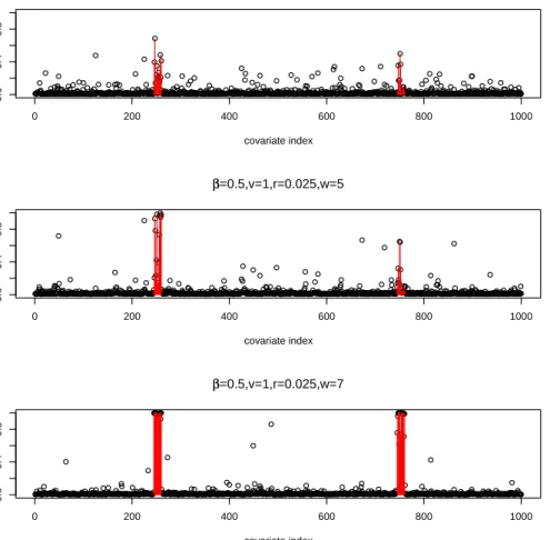
additive effects over two blocks of consecutive covariates. The true β used to generate the data is allowed to vary over {0.5,1,2}, and we experimented with Bayesian variable selection with varying levels of v, r, and w under the same stationary distribution π. For each setting of hyperparameters, we ran the Gibbs sampler 10 times with random start in γ. Each run has 100,000 iterations with the first 50,000 iterations as burnin. For 100,000 iterations with average posterior model size of 40, the complete procedure takes about 2.5 hours to run on a Sun Fire Unix V880 with 1200Mhz ultraSprac III CPU. In all of our experiments, the 10 simulations lead to highly similar posterior summary statistics, indicating convergence of the MCMC.
For high dimensional covariate spaces (m in thousands or more), the traditional posterior summary statistics of counting the occurrence of each particular posterior model is infeasible because any model is most likely to be sampled only once in a MCMC with workable length, as observed in our simulations. A natural alternative is to instead calculate the posterior marginal distribution of γi, P(γi = 1|Y), by dividing the number of iterations where γi = 1
over the total number of iterations excluding the burnin period. To compare between models, we can further compute the ROC curve as follows: only those covariates i with P(γi = 1|Y)
greater than a threshold are deemed positives, and those below the threshold are deemed negatives, then the ROC curve reflects the pair of (true positive rate, false positive rate)
● ● ●●●●●●● ● ● ●●●●●●●●●● ● ●●●●●●●●●●●●●●●●●● ● ● ● ●●● ● ● ● ● ●●●●●●●●●●●●●●●●●● ● ● ●●●●●●●● ● ●●●●●●●●●●● ● ●●●●●●●● ● ●●●●●●●●●●●●●●●●●●●●●●●● ● ●●●●● ● ● ●●●●●●●●●●●●●●●●●●● ● ●●●●●●●●●●●● ● ● ● ● ● ● ●●● ● ● ●●●●●●●●●●●●●●●●●●●●●●●●●●●●●●● ● ●●●●●●●●●●●●●●●●● ● ●●●●●●●●●●●●●●●●●●●● ● ● ● ● ● ● ● ● ● ● ●● ● ● ● ● ● ●●●●●●●●●● ● ●●●●●●●●●●●●●●●●●● ● ● ● ●●●●●●●● ● ●●●●●●●●●●●● ● ●●● ● ● ●●●●●● ● ●●●●●●●●●●●●●●●●●●●●●●●●●●●●●● ● ● ●●●●●●●●●●●●●●●●●●●●●●●●●●●●●●●●●●●●●●●●●●●●●●●●●●●●●●●●●●●●●●●● ● ● ●●●●● ● ● ●●●●●●●●●●●●● ● ● ● ●●●●●●●● ● ●●●● ● ● ● ●●●● ● ● ●●●●●●●●●●●●●●●●●●●●●●●●● ● ●●●●●●●●●●●●●●●●●●●●●●●●●●●●● ● ● ● ●●●●●●●●● ● ● ●●●●●●●●●●●●●●●● ● ● ● ● ●●●●●●●●● ● ●●●●●●●●●●● ● ● ●●●●●●●●●●●●●●●●●●●●●●●●●●●●●● ● ● ● ● ●●●●●●●●● ● ● ● ● ● ●●●●●●●●●●●●●●●●●●●●●●●●●●●●●●●●●● ● ● ● ●●●● ● ● ●●●●●●●●●●●●●●●●●●●●●●● ● ● ● ●●●●●●●●●● ● ●●●●●●● ● ● ●●●●●●●●●●●●●●●●●●●●●●●●●● ● ● ● ● ● ● ●●●●●●●●●●●●●●●●●●●●●●●●●●●●●●●●●●●●●●●●●●● ● ● ● ●●●●● ● ●●●●●●● ● ● ● ●● ●●●●●●●● ● ●● ● ● ● ● ● ●● ● ● ●●●●●●●●●●●●●●●●●● ● ●●●●●●●●●●●●●●●●●●●●●●●●●● ● ●●●●●●●●●●●●●●● ● ● ● ●●●●●●●●●●●●●●●●●●● ● ● ●●●●●●●●●●●●●● ● ● ●●●●●●●●●●●●●●●●●●●● ● ● ● ●●●●●●●●●●●●●●●●●● ● ● ●●●●●●●●●●●●●● ● ● ●●●● 0 200 400 600 800 1000 0.0 0.4 0.8 covariate index marginal probability ββ=0.5,v=1,r=0.025,w=1 ● ● ●●●●●●●●●●●●●●●●●●●●●●●●●●●●●●●●●●●●●● ●● ● ●●●●● ● ● ●●●●●●●●●●●●●●●●●●●●●● ● ● ● ●●●●●●●●●●●●●●●●●●●●●●●●●●●●●●●●●●●●●●●●●●●●●●●●●●●●●●●●●●●●●●●●●●●●●●●●●●●●●●●●●●●●●●●●● ● ● ●● ●●●●●●●●●●●●●●●●●●●●●●●●●●●●●●●●●●●●●● ● ●●●●●●●●●●●●●●●●● ● ●●● ● ● ●●●●●●●●●●●●●●● ● ● ● ● ● ● ● ● ● ● ● ● ● ● ● ● ● ●●●●●●●●●●●●●●● ● ●●●●●●●●●●●●●●●●● ● ●●●●●●●●●●●●●●●●●● ●● ●●●●●●●●●●●●●●●●●●●●●●●●●●●●●●●●●●●●●●●●●●●●●●●●●●●●●●●●●●●●●●●●●●●●●●●● ● ● ● ● ●●●●●●●●●●●●●●●●●●●●●●●●●●●●●●●● ● ● ● ● ●●●●●● ● ●●●●●●●●●●●●● ● ●●●●●●●●●●●●● ● ● ● ●●●●●●●●●●● ● ● ●●●●● ● ● ●●●●●●●●●●● ● ●●●●●●●●●●●●●●●●●●●●●●●●●●●●●●●●●●●●●●●●●●●●●●●●●●●●●●●●●● ● ● ● ●●●●●●●●●●●●●●●●● ● ●●●●● ● ● ●●●●●●●●●●●●●●●●●●●●●●●●●●●●●●●●●●● ● ● ● ● ●●●●●● ● ● ● ●●●●●●●●●●●●●●●●●●●● ● ●●●●●●●●●●●●●●● ● ●●●● ● ● ●●●●●●●●●●●●●●●●●●●●●●●●●●●●●●●●●●●●●● ● ●●●●● ● ● ●●●●●●●●●●●● ● ● ●●●●●●●●●●● ● ● ●● ● ● ● ●●●●●●●●● ● ● ●●●●●●●●●●●●●●●●●●●●●●●●●●●●●●●●●●●●●●●●● ●● ● ●●●●●● ● ●●●●●●●●●●● ● ● ●● ● ● ● ●●●●●●●●●●●●●●●●●●●●●●●●●●●●● ● ● ● ●●●●●●●●●●●●●●●●●●●●●●●●●●●●●●●●●●●●●●●●●●●●●●●●●●●●●●●●●●●●●●●●●●●●●●● ● ● ●●●●●●●●●●●●●●●●●●●●●●●●●●●●●●●●●●●●●●●●●●●●●●●●●●●●●●●●●●●●● ● ● 0 200 400 600 800 1000 0.0 0.4 0.8 covariate index marginal probability ββ=0.5,v=1,r=0.025,w=5 ● ● ●●●●●●●●●●●●●●●● ● ● ●●●●●●●●●●●●●●●●●●●●●●●●●●●●●●●●●●●●●●●●●●● ● ● ● ●●●●●●●●●●●●●●●●●●●●●●●●●●●●●●●●●●●●●●●●●●●●●●●●●●●●●●●●●●●●●●●●●●●●●●●●●●●●●●●●●●●●●●●●●●●●●●●●●●●●●●●●●●●●●●● ●● ● ●●●●●●●●●●●●●●●●●●●● ● ● ●●●●●●●●●●●●●●●●●●●●●●●●●●●●●● ● ● ●●●●●●●●●● ● ● ●●●●● ● ● ●●●●● ● ● ● ● ●●●●●●●●●● ● ●●●●●●●●●●●●●●●●●●●●●●●●●●●●●●●●●●●●●●●●●●●●●●●●●●●●●●●●●●●●●●●●●●●●●●●●●●●●●●●●●●●●●●●●●●●●●●●●●●●●●●●●●●●●●●●●●●●●●●●●● ● ● ●●● ● ● ●●●●●●●●●●●●●●●● ● ● ●●●●●●●●●●●●●●●●● ● ●●●●●●●●●●● ● ●● ● ● ●●●●●●●●● ● ● ● ●●●●●●●●●●●●●●●●●●●● ● ● ●●●●●●●●●●●●●●●●●●●●●●●●●●●●●●●●●●●●●●●●●●●●●●●●●●●●●●●●●●●●●●●●●●●●●● ● ●●●●●●●●●●●●●●●●●●●●●●●●●●●●●●●●●●●●●●●●●●●●●●●●●●●●●●●●●●●●●●●●●●●●●●●●●●●●●●●●●●●●●●●●●●●●●●●●●●●●●●●●●●●●●●●●● ● ●●●●●●●●●●●●●●●●●●●●●●●●●●●●●●●●●●●●●●●●●●●●●●●●●●●●●●●●●●●●●●●●●●●●●●●● ● ●●● ● ● ● ● ● ● ●●●● ● ● ● ●●●●●●●●●●●●●●●●●●●●●●●●●●●●●●●●●● ● ● ● ●●●●●●●●●●●●●●● ● ●●●●●●●●●●●●●●●●●●●●●●●●●●●●●●●●●●●●●●●●●●●●●●●●●●●●●●●●●●●●●●●●●●●●●●●●●●●●●●●●●●●●●●●●●●●●●●●●●●●●●●●●●●●●●●●●●●●●●●●●●●●●●●●●●●●●●●●●●●●●●●●●●●●●●●●●●●●●●●●●●●●●●● ● ● ●●●●●●●●●●●●●●●●●● 0 200 400 600 800 1000 0.0 0.4 0.8 covariate index marginal probability ββ=0.5,v=1,r=0.025,w=7
Figure 1. Marginal probability ofγ under simulation model (3.4) (smooth inγ)
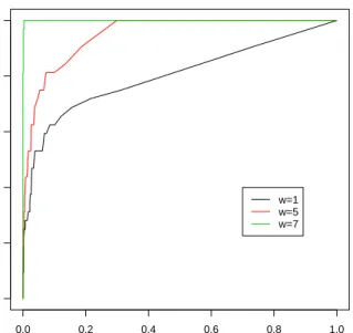
achieved by varying the calling threshold. The bigger area under the ROC curve (maximum 1), the better the discriminating power of the model.
Here we present the results where the signal is weak (β = 0.5). Figure 1 shows the posterior marginal probability ofγ with fixedv = 1,r =π1/π0 = 0.025, and varying w1 = 1,5,7, where
the indices of true γi = 1 are labeled by red lines. Figure 2 shows the corresponding ROC
curves. Note thatw1 = 1 corresponds to the case ofγi’s i.i.d.. It is quite clear from the results
that in this simple additive model the assumed Markov chain prior indeed yields significantly better results. For the easier tasks where the underlying models have stronger signal (larger
β), the improvement becomes even more pronounced. This pattern is consistently observed in each of our simulations.
Scenario 2: Smooth in X. It is intuitively obvious that in simulation model (3.4), a smoothed model fit performs better: The truth agrees with the model! We now study a more complicated scenario where the relationship between consecutive covariates is more subtle. We let Xk =
(Xk,1, . . . , Xk,m) be piecewise continuous:
Xk,i=δZkI(i∈[i∗−Lk,1, i∗+Lk,2]) +ξk,i, (3.5)
whereξk,i ∼N(0,1),Zk ∼Bernoulli(1/2), andLk,1 andLk,2 are independent Poisson random
0.0 0.2 0.4 0.6 0.8 1.0 0.0 0.2 0.4 0.6 0.8 1.0
ROC curve of different w (ββ=0.5,v=1,r=0.025)
False positive rate
True positive rate w=1
w=5 w=7
Figure 2. ROC curve under simulation model (3.4) (smooth inγ)
Lk,1 +Lk,2 covering location i∗. Then, let the response depend only on whether there is a
jump at i∗:
Yk∼βZk+k.
Hence,Yis related toXonly through the latent variableZ. Xmay or may not contain a jump near i∗, and since the jump involves the neighboring covariates as well, pooling information across adjacent covariates might aid in the determination of the value ofZk, and thus also in
the prediction of the value of Y.
It is quite clear that model (3.5) pose a much harder variable selection task than model (3.4) because of the extra noise introduced in X. This means a small underlying effect size (β) usually leads to poor performance of the Baysian variable selection procedure with any
w. However, as β increases, the models differ in performance.
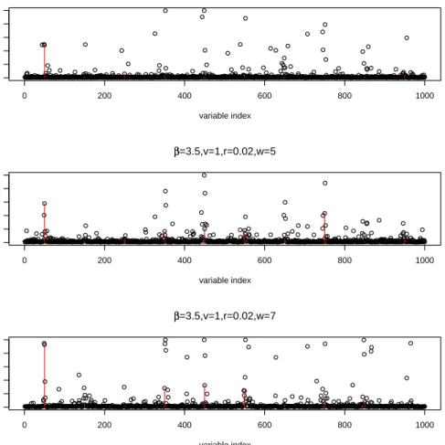
Here we present the results under model (3.5) with δ = 0.35, β = 3.5, and 10 spikes in
X, i∗ = (50,150,· · · ,950). Figure 3 shows the posterior marginal probability of γ with fixed
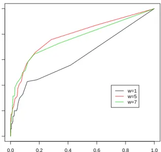
v = 1, r = 0.02 and varying w = 1,5,7. Figure 4 shows the corresponding ROC curves. The gain over a smoothed prior for γ is understandably less than that for the first simulation model. However, it is clear that when the jump size δ is small, pooling information across neighboring covariates can help significantly in identifying the location of i∗. An interesting feature shown in Figure 4 is that above certain value (> 1), larger w does not necessarily result in larger area under ROC curve. This is not surprising because the extra signal from pooling information over a large neighborhood under overly large wtends to be outpassed by the extra noise introduced at the same time.
● ● ●●●●●●●●●●●●●●●●●●●●●●●●●●●●●●●●●●●●●●●●● ● ● ●●● ● ● ●●●●●●● ● ● ●● ● ● ●●●●●●●●●●●●●●●●●●●●●●●●● ● ● ● ●●●●●●●●●●●●●●●●●●●●●●●●●●●●●●●●●● ● ● ●●●●●●●●●●●●●●●●●●●●●●●● ● ● ● ●●●●●●●●●●●●●●●●●●●●● ● ● ●●●●●●●●●●●●●●●●●●●●●●●●●●●●●●●●●●●●●●●●●●●●●●●●●●●●●●●●●●●●●●●●● ● ●●●●●●●●●●●●●●● ● ●●●●●●●●●●●●●●●●●●●●●●●●●●●●●●●●●●●●●●●●●●●●●●●●●●●●●●●●●●●●●●●●●● ● ●●●●●●●●● ● ● ●●●●●●●●●●●●●● ● ● ●●●●●●●●●●●●●●●●●●●●●●●●●●●●●●●●●●●●●●●●●●●●●●●●●●●●●●●●●●●●●●●●●● ● ● ●●●●●●●●●●●●●●●●●●●●●● ● ●●●● ● ● ● ●●● ● ● ●●●●●●●●●●●●●●●●●●●●●●●●●●●●●●●●●●●●●●●●●●●●●●●●●●● ● ●●●●●●●● ● ●●●●●●●●●●●●●●●●●●●●● ● ● ●●●● ● ● ● ●●●● ● ● ● ●●●●● ● ●●●●●●●●●●●●●●●●●●●●●●●●●●●●●●●●●●●● ● ●●●●●●●●●●●●●●●●● ● ●●●●●●●●●●●● ● ● ●●●●●●●●●● ● ●● ● ●● ● ● ● ● ● ● ● ●●●●● ● ● ●●●●● ● ●●●●●●●●●●●●●●●●●●● ●●●●●●●●●●●●●●●●●●●●●● ● ● ● ●●●●●●●●●●●●● ● ● ● ●●●●●●●●●●●●●●●●●●● ● ● ● ●●● ● ● ● ● ●●●●●●●●●●●●●●●●●●●●●● ● ●●●●●●● ● ● ●●●●●●●●● ●●●●●●●●●●●●●●●●●●●●●●●●●●●●●●●●●●●●●●●●●●●●●●●●● ● ● ● ● ●●●●●● ● ● ● ● ● ●●●●●● ● ●●●●●●●●●●●●●●●●●●● ● ● ●●●●●●●●●●●●●●●●●●●●●●●●●●●●●●●●●●●●●●●● ● ●●●●●●●●●●●●●●●●●●● ● ●●●●●● ● ●●●●●●●●●●●●●●●●●●●●●●●●●●●●●●●●●●●●●●●●●●●●● 0 200 400 600 800 1000 0.0 0.4 0.8 variable index marginal probability ββ=3.5,v=1,r=0.02,w=1 ● ● ●● ● ● ●●●●●●●●●●●●●●●●●●●●●●● ● ● ●●●●●●●●●●●● ● ● ●●● ● ● ● ● ●●● ● ●●●●●●●●●●●●●●●●●●●●●●●●●●●●●●●●●●●●●●●●●●●●●●●●●●●●●●●●●●●●●●●●●●●●●●●●●●●●●●●●●●●●●●●●●●●●●●● ● ● ● ●●●●●●●●●●●●●●●●●●●●●●●●● ● ●●●●●●●●●●●●●●●●●●●●●●●●●●●●●●●●●●●●●●●●●●●●●●●●●●●●●●●●●●●●●●●●●●●●●●●●●●●●●●●●●●●●●●●●●●●●●●●●●●●●●●●●●●●●●●●●●●●●●●●●● ● ● ●●●●●●●●●●●●●●●●●●●●●● ● ●●●●●●●●●● ● ●●●●● ● ● ●●●●● ● ● ● ● ●●●●●●●●●●●●●●●● ● ● ●●●●●●●●●●●●●●●●●●●●●●●●●●●●●●●●●● ● ● ● ●●●●● ● ●●●●● ●● ● ● ● ●●●●●●●●●●●●●●●●● ● ● ● ●● ●● ● ● ● ● ● ● ● ● ●●●●●● ● ● ● ●●●●●● ● ● ● ●●●●●●●●●●●●●●●●●●●●●●●●●●●●●●●●●●●●●●●●●● ● ●●●●●●●●●●●●●●●●●●●●● ● ● ●●●●●●●●● ●● ● ● ● ●●●●● ● ●● ● ●●●●●●●●●●●●●●●● ● ● ●●●●●●●●●●●●●●●●●●●●●●●●●●●●●●●●● ● ●●●●●●●●●●●●●●●●●●●●●●●●●●●●●●●● ● ● ● ● ● ●●●●●● ● ●●●●●●●●● ● ● ●●●●●●●●●●●● ● ● ●●●●●●●●●●●●●●●●●●●●●● ● ● ● ●●●●●●●●●●●●● ● ● ● ●●●●●●●●●●●●●●●●●●● ● ● ● ●● ● ● ● ● ● ●●●●●●●●●●●●●●●●●●●●●●●●●●●●●●●●●●●●●●●●●●●●●●●● ● ● ●●●●●●●●●●●●●●●●● ● ● ●●●●●●●●●●● ● ● ●●●●●●● ● ● ● ● ● ●●●●●● ● ● ● ●●●●●●●●● ● ● ●●●●●●●●●●●●●●●●● ● ● ●●●●●●●●●●●●●●●●●●●●●●●●●●●● ● ●●●●●●●●●●●●●●●●●●●●●●● ● ● ●●● ● ● ● ● ●●●●●● ● ● ● ●●●●●●●●●●●●●●●●●●●●●●●●●●●●●●●●●●●● ● ●●●●●● 0 200 400 600 800 1000 0.0 0.4 0.8 variable index marginal probability ββ=3.5,v=1,r=0.02,w=5 ● ● ●●●●●●●●●●●●●●●●●●●●●●●●●●●●●●●●●●●●●●●●●●●● ● ● ● ● ● ● ●●●●●●●●●●●●●●●●●●●●●●●●●●●●●●●●● ● ●●●●●● ● ●●●●●●●●●●●●●●●●●●●●●●●●●●●●●●●●●●●●●●●●●● ● ●● ● ●●●●●●●● ● ● ● ● ● ● ● ●●●●●●● ● ● ● ●●●●●●●●●●●●●●●●●●●●●●●●●●●●●●●●●●●● ● ● ●●●●●●●●●●●●●●●●●●●●●●●●●●●●●●●●●●●●●●●●●●●●●● ● ● ●●●●●●●●●●●●●●● ● ●●●●● ● ● ●●●●●●●●●●●●●●●●●●●●●●●●●●●●●●●●●●●●●●●●●●●●●●●●●●●●●●●●●●●●● ● ●●●●●●●●●●●●●● ● ● ● ● ●●●● ● ● ● ●●●●●●●●●●●●●●●●●●●●●●●●●●●●●●●●●●●●●●●●●●●● ● ● ● ● ●●●●●●●●●●●● ● ●●●●●●●●●●●●●●●●●●●●●●●●●●● ● ● ● ● ● ●● ● ●●●●●●●●●●●●●●●●●●●●●●●●●●●●●●●●●●●●●●●●●●●●●●●●●●●● ●● ●●●●●●●●●●●●●●●●●●●●●●●●●●●●●●●●●●●●● ● ● ● ● ● ● ● ●●●●● ● ●●● ●●●●●●●●●●●●●●●●●●●●●●●●●●●●●●●●●●●●●●●●●●●●●●●●●●●●●●●●●●●●●●● ● ● ● ●●●●●●●●●●●●●●●●●●●●● ● ● ●●●●●●●●●●●●●●●● ● ● ●●●●●●●●●●●●●●●●●●●● ● ● ● ●●●●●●●●●●●●● ● ● ● ●●●●●●●●●●●●●●●●●●●● ● ● ●●●●●●●● ● ● ●●● ● ● ● ●●● ● ● ● ● ● ● ● ●●●●●●●●●●●●●●●●●●●●●●●●●●● ● ● ●●●●●●●●●●●●●●●●●●●●●●●●●● ● ● ●●●●● ● ●●●●●●●●●●●●●●●●●●●●●●●● ● ● ● ● ● ● ●●●● ● ● ● ●●●●●●●● ● ● ● ●●●●●●●●●●●●●●●●● ● ● ●●●●●●●●●●●●●●●●●●●●●●●●●●●●●●●●●●●●●●●●●●●●●●●●●●●●●●●●●●●●●●●●●●● ● ●●●●●●●●● ● ● ●●●●●●●●●●●●●●●●●●●●●●●●●●●●●●●●●● 0 200 400 600 800 1000 0.0 0.4 0.8 variable index marginal probability ββ=3.5,v=1,r=0.02,w=7
Figure 3. Marginal probability ofγ under simulation model (3.5) (smooth inX)
3.1.5 Results on a Colorectal Cancer Data Set
The two simulation models in the last section reflect two different hypotheses for the rela-tionship between DNA copy number and cancer outcome. The first model, which we will call the “multiple-genes model”, reflects the hypothesis that the dosage level of multiple genes in an aberrant region in the genome contribute collectively to the cancer outcome. This type of model applies, for example, to the well-known effects of trisomy and contiguous gene dele-tion syndromes. Recently it has been hypothesized (Mitelman et al. (1997), Duesberg et al. (2005)) that the dosage effect of whole sets of genes also play an important role in cancer. Alternatively, the second “one-gene” model applies to the case where the aberrant region is caused by the selection for a single oncogene, with the other genes in the region having no or little effect on the outcome. This type of model has been proposed to explain many cases of recurrent escalating amplifications in neoplasms such as the ERBB2 region in breast cancer. As we have shown using our simulation study, both models could potentially benefit from the linear Markov prior on γ. However, the size of the improvement depends both on the error structure in the data as well as the strength of the hypothesized effect.
As an example, we analyze the BAC array-CGH data from colorectal liver metastasis re-sected from 50 patients, taken from Mehta et al. (2005). For this data set, clinical variables
0.0 0.2 0.4 0.6 0.8 1.0 0.0 0.2 0.4 0.6 0.8 1.0
ROC curve of different w (ββ=3.5,v=1,r=0.02)
False positive rate
True positive rate w=1
w=5 w=7
Figure 4. ROC curve under simulation model (3.5) (smooth inX)
such as the overall survival time of the patient are available. The covariates are the
mea-surements of DNA copy number at 2153 (m) locations along the whole genome. Our goal
is to identify regions of the genome that have prognostic value in predicting overall survival. The survival time for this data set is fully observed (no censoring), thus we model it by the Gaussian distribution. We applied a square root transform to the survival time to stabilize variance.
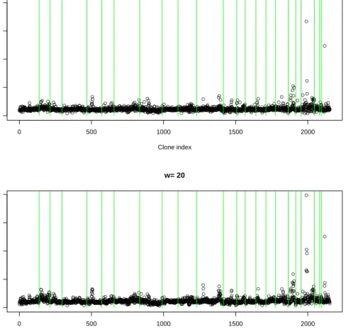
We use the linear Markov chain prior with w1 ∈ {0,20}to analyze this data. The MCMC
chain ran for 150000 iterations, of which the first 100000 iterations were used as burn-in. The results from 10 random restarts confirmed the convergence of the chain. Figure 5 shows the posterior marginal probabilities for γi plotted against location in the genome. For this
data set, the most prominent spike in the posterior marginal probabilities has a height ≈0.4, indicating that there is no single genomic location which has a strong correlation with survival. This is consistent with the conclusions of Mehta et al. (2005), who found that, although the total fraction of genome altered is a significant independent predictor of survival, no single clone has a significant independent effect.
However, quite a few regions have marginal posterior probabilities that rise above the bulk. This is especially noticeable when one zooms in on the marginal probability plots for each chromosome separately (Figure 6). The mean posterior model size, to the nearest integer, is 53 for both values ofw. The mean ofP(γi|Y) is 0.0245 and 0.0246 respectively forw1 = 0,20,
which are both roughly equal to 53/2153 = 0.0246, the marginal posterior probability for each
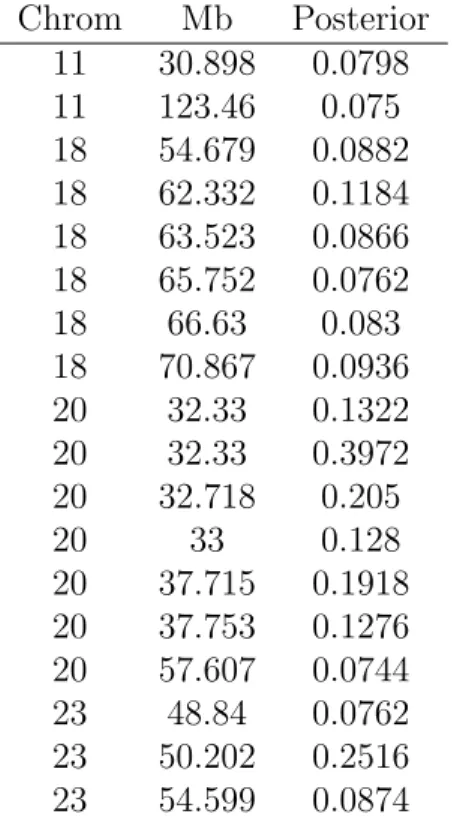
γi assuming that all covariates are a posteriori equally likely to be in the model. Table 1 lists
the clones whose posterior marginal probability are three fold above the mean.
For colorectal carcinoma, several regions of the genome have already been confirmed by numerous studies to have good prognostic value in predicting survival. The two regions that have received the most attention are chromosome arm 18q and 20q, both of which figure
● ● ●●●●●●● ● ● ● ●●●●●●●●●●●●●●●●●●●●●●●●●●● ● ● ●●●●●●●●●●●●●●●●●●●●●●●●●●●● ● ● ● ● ● ● ● ●●● ● ● ●●●●●●●●●●●●●●●●●●●●●●●●●●●●●●●●●●●●●●●●●●● ● ●●●●●●● ● ● ● ●●●●●●●●●●●●●● ● ● ● ● ● ●●● ● ● ●●●●●●●●●●●●●●●●●●●●●●●●●●●●●●●●●● ● ● ● ● ● ● ●●●●●● ● ● ● ● ● ● ● ● ●●●●●●●●●●●●●●●●●●●●●●● ● ● ●●●● ● ● ● ● ● ● ●●●●●●●●●●●●●●●●●●●●●●●●●●●●●●●●●●●●●●●●●●●●●●●●●● ● ● ● ● ●●●●●●●●●●●●●●●●●●●●●●●● ●●●●● ● ● ● ● ● ●●●●●●●●●●●●●●●●●●●●●●●●●●●●●● ● ● ● ● ● ●●●●● ● ● ● ● ●●●●●●●●●● ●●● ● ● ●●●●●●● ● ● ● ●●●●●●●●●●●●●●●●●●●●●●●●●●●●●●●●●●●●●●●●●●● ● ●●●●●●●●●●●●●●●●●●●●●●●●●●●●●●●●● ● ● ●●●●●●●●●●●●●●●● ● ● ● ●● ● ● ● ●●●●●●●●●●●●●●●●●●●●●●●●●●●●●●●●●●●●●●●●●●●●●●●●●●●●●●●●●●●●●●●●●●●●●●●●●●●●● ● ● ●●●●●●●● ● ● ●●● ● ●●●●●●●●●●●●●●●●●●●●●●●●●● ● ● ● ● ●●●● ● ●●●●● ● ● ● ● ● ●●●●●●●●●●●●●●●●●●●●●●●●●●●●●●●●●●●●●●●●●●●●●●●●●● ● ● ● ● ●●●●●●●●●●●●●●●●●●●●●●●●●● ● ● ● ●●●●●●●●●●●●●●● ●●● ● ● ●● ● ● ● ● ● ● ● ● ●●●●●●●●● ● ●●●●●●●●●●●●●●●●●●●● ● ● ● ● ●●● ● ● ● ● ● ● ● ●●●●●●●●●●●●●●●●●●●● ●●●●●● ● ● ● ●●●●●●● ● ● ● ●● ● ● ● ●●●●●●● ● ● ● ●●●●●●●●● ● ●●●●● ●● ● ● ● ●●●●●●●●●● ● ● ● ● ●●● ● ● ●● ● ● ● ●●●●●●●●●●●●●●●●●●●●●●●●●● ● ● ● ● ●●●●●●●●●●●●●●●●●●●●● ● ● ● ● ● ● ● ● ●●● ● ● ●● ● ● ● ●●●●●●●●●●●●●●●●●●●● ●●● ● ● ●●●●●●● ● ● ●●●●●●●●●●●●●●●●●●●●●●●●●●●●●●●●●●●●●●●●●●●●●●●●●●●●●●●●●●●●●●●●●●●●●●●●●●●●●●●●●●●●●●●●●● ● ● ● ● ●●●●●●●●●●●●●●●●●●●●●●●●● ● ● ● ● ●●●●●●●●●●●●●●●●●●●●●●●●●●●●●●●●●●●●●●●●●●●●●●●●●●●●● ● ●●●●●● ● ● ● ● ●●● ● ● ●●● ● ● ●●● ● ● ●●●●●●●●●●●●●●●●●●●●●●●●●●●●●●●●●●●●●●●●●●●●●●●●●● ● ● ● ● ●●●●●●●●●●● ● ● ● ● ●● ● ● ●●●●●●●● ● ● ●●●●●●●●●●●●●●●●●●●●●● ● ● ● ●●●●●●●●●●●● ● ● ● ●●●●●●●● ● ●●●●●●●●●●●●●●●●●●●●●●●●●●●●●●●●●●●●●●●●●●● ● ● ●● ● ● ● ●●●●●● ● ● ● ●●●●●●●●●●●●●●●●● ● ● ● ●●●●●●●●●●●●●●●●●●●●●● ● ● ● ●● ● ● ● ●●●●●●●●●●●●●● ●●●●●●● ● ● ● ● ● ● ● ● ●●●●●●●●●●●●●●●●●●●●●●●● ● ●●●●●● ● ● ● ● ● ● ● ● ●●●●●●●●●●●●●● ● ●●●●●●●●●●●●●●●●●●●●●●●● ● ● ● ● ● ● ●●●●●● ● ● ● ●●●●●●●●●●●●●●●●●●●●●●●●●●●●●●●●●●●● ● ● ● ● ● ● ● ● ● ●●●●●●●●●●●●●●●●●● ● ●●●●●●●●●●●● ● ● ● ● ● ● ● ● ●● ● ● ● ●●●●●●●●●●●●●●●●●●●●●●●●● ● ● ● ● ●●●●●●●●●●●●●●●●●●●●●● ● ● ● ●●●●●●●●●●●●●●●●●●●●●● ● ● ●●●●●●●●●●●●●●●●●●●●●●●●●●●●●●● ● ● ● ● ●●●●●●●●●●●●●●●●●●●●●●●●●●● ● ● ●●●●●●●●●●●●●●●●●●● ● ●●●●●●●● ● ● ●●●●●●● ● ● ● ●●●●●●●●●●●●●●●●●● ● ● ● ● ● ● ● ● ● ● ● ●●●●●●●●●● ●● ● ● ● ●●●●●●●● ● ● ●●● ● ● ● ● ● ● ● ● ● ● ● ●●●●●●● ● ● ● ●●●●●●●●●● ● ● ● ● ● ●●●● ● ●●●●●●●●●●●●●●●●●● ● ● ●●●● ●● ● ● ● ●●●●● ●● ● ● ● ● ● ● ● ● ●●● ● ● ●● ● ● ● ● ● ● ● ● ● ● ● ● ● ● ● ● ● ● ●●●●● ● ● ● ● ● ● ● ● ● ● ● ● ● ● ● ● ● ● ● ● ● ● ● ● ● ● ● ● ● ● ● ● ● ● ●●● ● ● ●●●●●●● ● ● ● ●●●●●●●●●●●●●●●●●●●●●●●●● ● ● ● ● ●●●● ● ●●●●●●●●●●●●●●●●●●●●● ● ● ● ● ●●●●● ●● ● ● ●●●●● ●●●●●● ● ● ● ● ●●●●● ●●●● 0 500 1000 1500 2000 0.0 0.1 0.2 0.3 0.4 Clone index Posterior marginal w= 1 ● ● ●●●●●●●●●● ●●●●●●● ● ● ● ●●●●●●●●● ● ●●●●●●●●●●●●●●●●●●●●●●●●●●●●●●●●●●●●● ● ● ●● ● ● ● ●●●●●●●●●●●●●●●●●●●●●●●●●●●●●●●●●●●●●●●●●●●●●●●●● ●●●●●●●●●●●●●●●●●●●●●●●● ● ● ● ● ● ●●● ● ● ● ● ● ● ● ●●●●●●●●●●●● ● ● ● ●●●●●●●●●●●●●●●●●● ● ● ●●●●●● ● ● ● ● ● ● ● ● ●●●●●●●●●●●●●●●●●●●●●●● ● ● ●●●● ● ● ● ● ● ● ●●●●●●●●●●●●●●●●●●●●●●●●●●●●●●●●●●●●●●●●●●●●●●●●●●●●●●●●●●●●●●●●●●●●●●●●●●●●●●●●●● ● ●●●●●● ● ● ● ● ●●●●●●●●●●●●●●●●●●●●●●●●●●●●●● ●● ● ● ●●●●●●●●●●●●●●● ●●●●●●●●●●●●●●●●●●●●●●●●●●●●● ● ●●●●●●●●●●●●●●●●●●●●●●●●●●●● ● ●●●●●●●●●●● ● ● ● ● ●●●●●●●●●●●●●●●●●●●●●●●●●●●●●●●●●●●●●● ● ●●●● ● ●●●●●●●● ● ● ●●●●●●●●●●●●●●●●●●●●●●●●●●●●●●●●●●●●●●●●●●●● ●●●●●●●●●●●●●●●●●●●●●●● ● ● ●●● ● ● ●● ● ● ● ●●●●●●●●●●●●●●●●●●●●●●●●●●●●●●●●●● ●●●● ● ●●●●● ● ● ● ● ● ●●●●●●●●●●●●●●●●●●●●●●●●●●●●●●●●●●●●●●●●●●●●●●●●●●●●●●●●●●●●●●● ● ●●●●●●●●●●●●●●●●●●●●●●●●●●●●●●●●●●●●● ● ● ●●●● ● ●●●●●●●●●●●●●●● ●●●●●●●●●● ● ● ● ● ●●●●● ●● ● ● ● ●●●●●● ● ● ● ● ●●●● ● ● ● ● ● ● ●●●● ● ●●●●●●●●●●● ● ● ● ●●●●●●●●●●●● ● ● ● ●●●●● ●●●●●●●●●●●●●● ● ● ● ● ● ● ●●●●●●●●●●●●●●● ● ● ● ● ●●● ● ● ●●●● ● ●●●●●●●●●●●● ● ● ● ●●●●●●●●●●●●●●●●●●●●●●●●●●●●●●●●●●●●●●●●●●●●●● ● ● ● ●●●●●●●●●●●●●●●●●●●●●●●●●●●●●●●●●●●●● ● ● ●●●●●●●●●●●●●●●●●●●●●●●●●●●●●●●●●●●●●●●●●●●●●●●●●●● ● ● ● ●●●●●●●●●●●●●●●●●●●●●●●●●●●●●●●●●●●●●●●●●●●●●●●●●●●●●●●●●●●●●●●●● ● ● ● ● ●●●●●●●●●●●●●●●●●●●●●●●●●●●●●●●●●●●●●●●●● ● ● ● ●●●●●●●●● ● ●●● ● ● ●● ● ● ● ●●●● ● ●●●●●●●●●●●●●●●●●●●●●●●●●●●●●●●●●●●●●●●●●●●●●●●●●●●●●●●●●●● ● ● ● ● ● ●●●●●●●●●●●●●● ● ● ● ● ● ●●●●●●●●●●●●● ● ● ●●●●●●●●●●●●●●●●●●●●●●●●●●●●●●●●●●●●●●●●●●● ● ●●●●●●●●●●●●●●●●●● ● ● ●●●●●●●●●●●●●●●●●●●●●●● ● ● ●● ● ● ● ●●●●●● ● ● ● ●●●●● ●●●●●●●●●●●●●●●●●●●●●●●●●●●●●●●●●●●●●● ● ● ●● ● ● ● ●●●●●●●●●●●●●●●●●●●●●●● ● ● ● ● ● ● ●●●●●●● ● ● ● ●●●●●●●●●●●●●●●●●●●●● ● ● ● ● ● ● ● ● ●●●●●●●●●●●●●●●●●●●●●●●●●●●●●●●●●●●●●●●●●●●●●●●●●●● ● ● ● ●●●●●●●●●●●●●●●●●●●●●●●●●●●●●●●●●●●●●●●●●●●●●●●●●●●●●●●●●●●●●●●●●●●●●●●●●●●●●●●●●●●●●● ● ● ● ●●●●●●●●●●●●●●●●●●●●●●●●● ● ● ● ● ●●●●●●●●●●●●●●●●●●●●●●●●●●●●●●●●●●●●●●●●●● ● ● ● ●●●●●●●●●●●●●●●●●●●●●● ● ● ●●●●●●●●●●● ● ● ● ● ●●●●● ●●●●●●●●●●●●●●●●●●●●● ● ● ● ●●●●●●●●●●●●●●●●●●● ● ●●●●●●●● ● ● ●● ● ● ● ●● ● ● ● ●●●● ● ●●●●●●●●●●●●●● ● ● ● ● ● ●●●●●●●●●●●●●●● ●●● ● ● ●●●●●●●● ● ● ●● ● ● ● ●● ● ● ● ● ● ● ● ●●●●●●●●●●● ● ● ● ● ●●●●● ● ● ● ● ● ●●●●●●●●●●●●●●●●●●● ● ●●●●●●●● ● ●● ● ● ● ●●●●●●●●●● ● ● ● ● ● ●●● ● ● ● ● ● ● ● ● ● ● ● ● ● ● ● ● ● ● ● ● ● ● ●●●●●● ● ● ● ● ● ● ● ● ●●●● ● ●● ● ● ● ●●● ● ● ●● ● ● ● ● ● ● ● ● ●●●●●●●●●●●● ● ● ● ●●● ● ● ●●●●●●●●●●●●●●●●●●●● ● ● ● ● ●●●●● ●●●●●●●●●●●●●●●●●●●● ● ● ● ● ● ●●●●● ●● ● ● ●●●●●●●●●●● ● ● ● ● ●●●●●●●●● 0 500 1000 1500 2000 0.0 0.1 0.2 0.3 0.4 Clone index Posterior marginal w= 20
Figure 5. Marginal probability ofγ for Mehta et al. colorectal cancer data.
prominently in Table 1. First, consider chromosome arm 18q. Several retrospective studies have identified correlations between loss of heterozygosity events in this region and reduced survival for patients with colorectal carcinoma. The effect is not always strong, as other studies have failed to identify this correlation. The evidence is strongest in the 18q21 region, which contains several cancer related genes, including DCC (deleted in colorectal carcinoma gene) and SMAD2 and SMAD4 (mothers against decapentaplegic homologue 2 and 4). However, it has been hypothesized by (Ji et al. 2007) that other candidate colorectal cancer genes may reside in this area which also provide good prognosis value.
Next, consider chromosome arm 20q13, which has been identified in breast and ovarian cancer with speculations about prognostic significance. In the case of colorectal carcinoma, several studies have reported amplifications in the 20q11-13 region and have found correlation between amplification in this region with worse outcomes.
For any value of w1 ∈(1,20), the chromosomal regions 18q21 and 20q13 contain the clones
with the highest posterior marginal probabilities. The posterior marginal probability increases slightly but steadily with increase in w1. Also worth noting is chromosome 11, which has also
been linked with poor prognosis in Tagawa et al. (1997). This region is noticeably more separated from the baseline probability of 0.0254 forw1 = 20.
● ● ● ●●●●● ●●●●● ● ●●●●●●●●●●● ● ●● ● ●●●●● ●●●● ● ● ● ●● ● ● ● ● ●●● ● ●●●●● ● ●●●● ●●●●●● ● ●●● ●● ●● ●●●● ●● ● ●●● ●●●●●●●● ●● ● ●● ●●●●●● ● ●● ●●● ● ● ● ●●● ● ●●● ● ● ●●●●●●● ●● ●● ●●● ● ● ● ●●● ● ● ●●●●●● ● ● ● ● ● ● ● ● ●● ●●●● ● ● ● ●●●●● ● ●● ● ● ●●● ●●● ● 0 50 100 150 0.01 0.04 0.07 Mb Posterior marginal Chromosome 11 ●●●● ●●●●●● ● ●●● ●● ● ● ● ● ● ● ●● ● ● ● ● ● ● ● ● ● ● ●● ●● ● ● ● ● ●●● ● ● ●● ●● 0 20 40 60 80 0.02 0.08 Mb Posterior marginal Chromosome 18 ●●● ●●●●●●●●●●●● ●●● ●●●●●●● ● ●● ●●●● ●●●● ● ● ● ● ● ● ●●●●●●● ●●●●●●●●● ●●●●●●●●● ●●●●● ●●●●●● ●●● ●●●●● ●● ●● ●●● 0 10 20 30 40 50 60 0.0 0.2 0.4 Mb Posterior marginal Chromosome 20
Figure 6. Chromosomes 11, 18, and 20 which contain regions of higher than 3 fold increase in posterior marginal probability than average.
Note that the simulation studies in the previous section show that the gain obtained from increased wis larger under the multiple-gene hypothesis than under the one-gene hypothesis, and that under the one-gene hypothesis the gain is larger if the separation between states (δ/σX) is small. Hence, the similarity of results between w1 = 0 and w1 = 20 may be due to
the high signal/noise ratio of the array-CGH data, the small effect size, or both.
3.2
DNA motif finding: hypercube prior
3.2.1 Background of Application
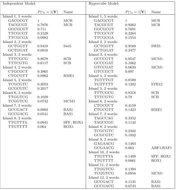
Transcription factors are proteins that regulate gene expression by binding to its surrounding sequence in the genome. Transcription factor binding sites (TFBS) usually contain low-entropy patterns called motifs. An important problem in biology is the modeling of the relationship between expression level of genes and the repertoire of motifs in their promoter sequences. Regression models have been applied to this problem in studies such as Bussemaker et al. (2001), Conlon et al. (2003), Zhang et al. (2007).
Transcription factors are usually degenerate, in the sense that words which are close to-gether in Hamming distance are more likely to be alternative binding sites for the same