Knowledge Base K Models to Support Trade-offs
for Self-adaptation using Markov Processes
Luis H. Garcia Paucar
SEA, ALICE, SARI, Aston University, UK email: [email protected]
Nelly Bencomo
SEA,SARI, Aston University, UK email: [email protected]
Abstract—Runtime models support decision-making and rea-soning for self-adaptation based on both design-time knowledge and information that may emerge at runtime. In this paper, we demonstrate a novel use of Partially Observable Markov Decision Processes (POMDPs) as runtime models to support the decision-making of a Self Adaptive System (SAS) in the context of the MAPE-K loop. The trade-off between the non-functional requirements (NFRs) has been embodied as a POMDP in the context of the MAPE-K loop. Using Bayesian learning, the levels of satisficement of the NFRs are inferred and updated during execution in the form of runtime models in the Knowledge Base. We evaluate our work with a case study of the networking application domain.
Index Terms—Runtime models, non-functional requirements, uncertainty, self-adaptation, decision-making, Markov Processes
I. INTRODUCTION
Runtime models can be defined as abstract representations of a system, including its structure and behaviour, which exist alongside the given system during the actual execution time [6]. Significant advances have been made in applying models at runtime, most notably in adaptive systems [3]. How-ever research challenges still prevail [4]. For example, further techniques to deal with uncertainty [11] and incompleteness of information from systems and their environment are needed for building future software systems [1], [9]. Techniques to update runtime models when more information and knowledge become available can proof to be suitable. Recent progress in machine learning [5], including Bayesian learning and inference, is key to enable access to information at runtime, to dynamically feed the models and keep them up-to-date [15]. In [15] we casted the decision-making problem of a self-adaptive system (SAS) and the trade-off of the quality properties such as of reliability and energy efficiency (a.k.a. non-functional requirements -NFRs) in terms of a POMDP decision problem. Based of these partial results the novel contribution of this paper is an architecture that leverages the different activities of the MAPE-K loop [29] to support decision-making in a SAS. We demonstrate how according to evidence collected at runtime from the monitoring infrastructure and Bayesian inference, the runtime models (i.e. runtime K models) kept as part of the Knowledge Base in the MAPE-K loop, can be updated accordingly to therefore underpin decision-making. We also demonstrate how once the runtime K models are changed, appropriate self-adaptations are generated, which are finally reflected on the managed system, which will better satisfice the requirements.
In our approach, a POMDP model is used as a runtime K model. The decision-making supported by the POMDP model is reflected on a managed system to therefore improve the levels of satisficement and according to the service level agree-ments (SLAs). Our experiagree-ments show how dynamic changes of the environment update the POMDP model to reflect the new conditions to, therefore, provide better informed decision-making than if the approached had not been used.
The paper is organised as follows. Section 2 describes the Research Baseline we have used to develop the ideas. Section 3 presents the runtime model POMDP and how it underpin decision-making under uncertainty for self-adaptation. Section 4 describes the software architecture based on the MAPE-K loop and runtime models. Section 5 describes experiments to explain and evaluate the contributions. In Section 6 related work is studied. Finally, Section 7 outlines the conclusions and future work.
II. RESEARCHBASELINE
A. POMDPs
POMDPs allow rational decision-making under uncertainty in changing environments [17]. A POMDP model can be specified as a 6-tuple(S, A, Z, T, O, R), where:
• S, A and Zrepresents the system’s state space, action space and observation space, respectively [2]. At each time step, the system takes actiona∈A to move from a states∈S
tos0 ∈S to eventually receive an observation z∈Z. • T:SxAxS→[0,1] is the transition function. It is a
condi-tional probability function T (s, a, s’ ) = P(s’|s, a) where at each time step, the system takes actiona ∈A to move from a states∈S tos0∈S.
• O:SxAxZ→[0,1]is the observation function. It describes the conditional probability function O(s’, a, z) = P(z|s’, a) of observing z ∈ Z when action a is performed and the resulting state iss0. It models noisy sensor observations. • R: SxA→R(s,a) is the reward function. The system gets a
rewardR(s, a)for taking actionaunder the current state s. In a POMDP, the system’s states are not directly observable. Instead, a belief, i.e. a probability distribution over possible states is maintained. The next step is to choose an action based on the current belief, i.e. to use apolicy. In terms of a POMDP, a policy defines a mapping that specifies the actiona=π(b) at beliefb. The goal is to choose an action that maximise the expected value as is shown below:
Vπ(b) =E(
∞
X
t=0
γtR(st, π(bt))|b0=b) (1) The constantγ∈[0,1)is the discount factor, which expresses preferences for immediate rewards over future ones. POMDPs provide support for decision-making over time, using partial knowledge of the states s∈S of a running system based on runtime evidence (i.e., observations z∈Z). In our work, the system’s state is the current satisficement level of its NFRs. B. MAPE-K loop
Self Adaptive Systems (SASs) [9], [10] can be implemented with an autonomous manager that steers the adaptation with a feedback control loop known as the MAPE-K feedback loop [29]. (M) stands for the monitoring process of the managed elements. It defines the frequency at which the data must be acquired.(A)represents theanalysisof the monitored data, which could require filtering actions either because of noise on the monitored data or because it cannot be used directly from its raw monitored values.(P)stands forplanning actions that implies the computation of the control law using the knowledge of the system held in the model.(E)represents theexecutionof the planned action. It consists of changing the value of the actuator(s) in a SAS at a frequency which is most often equivalent to the sampling frequency of the monitoring phase [25]. A MAPE-K loop also stores Knowledge (K) required for decision-making in a Knowledge Base (KB).
III. POMDPMODEL FORDECISION-MAKINGTRADE-OFF
A. Motivating example
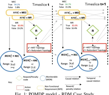
As an example to demonstrate the architecture and decision-making supported by using runtime models, let us consider the case of the Remote Data Mirroring (RDM) self-adaptive system (SAS). The RDM system is composed of data servers and network links. It must replicate and distribute data in an efficient manner by minimizing consumed bandwidth and providing assurance that distributed data is not lost or cor-rupted [16], [22]. The RDM system can be configured by using two different topologies: minimum spanning tree (MST) and redundant topology (RT). Both configurations allow the system selectively activate and deactivate network links to change its overall topology at runtime [13]. Fig. 1 presents the POMDP model of the RDM SAS for an IT network which has been used as a case study in [20].
The RDM SAS self-adapts by reconfiguring itself at runtime according to the changes in its environment, which may include either delayed or dropped messages and network link failures. Each network link in the RDM system brings upon an operational cost and has a measurable throughput, latency, and loss rate. The performance and reliability of the RDM system are determined by the following trade-off: (a) an RT topology offers a higher level of reliability than MST topologies. (b) However, the costs of maintaining a non-stop RT topology may be prohibitive in given contexts. Each configuration provides its own levels of reliability and energy costs which are taken into account while estimating the levels of satisficement of the NFRs observed: the Maximization of Reliability (MR) and the
Fig. 1: POMDP model - RDM Case Study Minimization of Energy Consumption (MEC).
The states of the NFRs are not directly observable. We obtain observations about their states by using monitoring variables (called MON variables). Two MON variables REC=“Ranges of Energy Consumption” (i.e., REC <x, REC in [x,y) and REC>=y) and ANL=“Active Network Links” (i.e., ANL<r, ANL in [r,s) and ANL>=s) are specified in the RDM system (see Fig. 1). The values x, y, r and s represent range boundaries for the variables REC and ANL. In the case of REC, the lower the monitored values, the greater the satisficement of MEC. Conversely, in the case of ANL, the higher the monitored values, the greater the satisficement of MR.
B. NFRs and satisficement values
Using a monitoring infrastructure (See MON variables in Fig. 1), observations are obtained that provide partial in-formation about the satisficement level of the NFRs. The observations are used to calculate the conditional probability distributions about the satisficement level of the NFRs (i.e. belief). For instance, in Fig. 1, given the previous adaptation action At and the previous N F Rt state, the probability
distribution for the satisficement of MEC at time slice t+1 is represented by:
P(MECt+1=True|NFRt,At) and P(MECt+1=False|NFRt,At)
Note that the higher the probability
P(MECt+1=True|NFRt,At), the higher the satisficement
level of MEC.
C. Approach for modeling NFRs trade-off in POMDPs The use of POMDPs allows the specification of NFRs in terms of a POMDP model. Such as specification is RE-STORM [15]. Next, the transition and observation functions of a POMDP in terms of the system’s NFRs are explained.
1) NFRs and the POMDP transition function: In a POMDP, the transition function T (s, a, s’ ) = P(s’|s, a) represents the probability of the system making a transition from state s to state s’ when actionais executed in states. The next definition allows us to represent the transition function in a POMDP in
relation to the belief (i.e. satisficement level) of the NFRs in a system.
Definition 1. The transition function T (s, a, s’ ) = P(s’|s, a), represents a system taking an action ’a’ under the current satisficement level of its related NFRs to update the next time slice with a new satisficement level of its NFRs.
Based on the previous definition, we can derive a transition function based on the NFRs of a system:
T(s, a, s0) =P(N F R0(1)...N F R0(n)|N F R(1)...N F R(n), A) (2)
Where N F R(i) and N F R0(i) represent the non-functional requirement “i” at the time slices t and t+1 respectively, ∀i ∈ [1, n]. By using Bayes’ theorem [24], the transition
function can also be factored into a product of conditional distributions. Let’s apply this concept in our RDM example. In Fig. 1, we observe that the non-functional requirements MEC and MR are influenced by the previous action at time slice t, but also by the previous state of MEC and MR i.e. they are interdependent. The factored transition function for this example is:
T(s, a, s0) =P(M EC0|M EC, M R, a)
P(M R0|M EC, M R, a) (3) As an example, the conditional probability table (CPT) for the transition function of MR is presented below in Table I.
TABLE I: CPT MR: P(MR’|MEC,MR,a)
2) Monitoring (MON) variables and the POMDP observation function: MON variables provide the observations required for runtime monitoring of the satisficement level of the NFRs. In a POMDP, the MON variables are represented as observations z from the environment. The next definition allows us to represent the observation function O(s’, a, z) = P(z|s’, a) of a POMDP in relation to the MON variables.
Definition 2. O(s’, a, z) = P(z|s’, a) represents a system that gets observation values z, from its monitoring variables, under the current satisficement level of their related NFRs and after taking action ’a’ in the previous time slice.
The observation function derived from definition 2, is repre-sented as follows:
O(z, a, s0) =P(M ON1|N F R1...N F Rn, A)
P(M ON2|N F R2...N F Rn, A)... P(M ONl|N F Rn...N F Rn, A)
(4)
WhereM ON(j)represents the MON variable “j” at the time slice t+1, ∀j ∈[1, l]. In the RDM example, the NFRs: MEC
Fig. 2: Runtime K models and Managed System and MR affect the MON variables Range of Energy Consump-tion (REC) and Active Network Links (ANL) respectively. The factored observation function for this example is:
O(z, a, s0) =P(REC|M EC0, A)P(AN L|M R0, A) (5) As an example, the conditional probabilities for the MON variable ANL is shown below in Table II.
TABLE II: CPT REC: P(REC|MEC’,a)
IV. MAPE-KANDPOMDPMODEL FOR DECISION-MAKING IN SELF-ADAPTATION
The different activities of the MAPE-K loop using POMDPs are as follows:
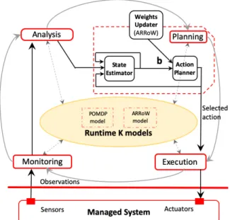
• Monitoring. The MON variables REC and ANL are mon-itored at runtime. They provide evidence to compute the probability distributions that represent the current satisfice-ment of the NFRs i.e. Minimization of Energy Consumption (MEC) and Maximization of Reliability (MR) respectively. • Analysis. Any required data transformation to enable data to be used at the planning phase (See Fig. 2) should be performed at this step. For example, whilst REC can be directly observed by sensors, ANL is computed using a reachability algorithm [28] that examines which RDM nodes can be reached by traversing active network links [22]. • Planning. We use online POMDP planning [23] to choose
the best action under the current state of the RDM system. Online POMDP planning is a technique that interleaves planning with plan execution: at each time slice, the system searches for an optimal action a∈A at the current belief b. It then executes the chosen action immediately [31]. • Execution Once an action has been selected, it is then
state s’ with probability T (s, a, s’ ) = P(s’|s, a) and receives an observation z∈Z with probability O(s’, a, z) = P(z|s’, a). It also receives a real-valued reward R(s,a).
• Knowledge Management From three inputs: (i) the observed monitored values, (ii) the actiona∈Aand (iii) the previous beliefb(See Fig. 2, inputs of thestate estimatormodule), the state estimator infers the current belief b, i.e., the current probability distributions about the satisficement of the NFRs MEC and MR. The state estimator updates the beliefbusing Bayes’ rule [31]. As a result of updating the belief b and based on the “memoryless property” of a Markov process [23] over time, the POMDP model infers the satisficement of the NFRs involved.
A. Details on the planning activity
We use the DESPOT algorithm [31] as the planner of our proposal. Two main steps are part of the planning activity:
1) Build a DESPOT tree to project future evolutions of NFRs: The planner considers future evolutions of the satis-ficement of the NFRs to decide the next action a∈A, i.e. to reason about long-term effects of immediate actions [26].
2) Select an optimal actiona∈A: The Bellman’s principal of optimality [24] is shown in equation (6) and is applied to a DESPOT tree to choose the best action:
V∗(b0) = max a∈A ( X s∈S b(s)R(s, a) +γX z∈Z p(z|b, a)V∗(r(b, a, z)) ) (6)
The algorithm searches the DESPOT tree with root at the current belief b0. The search is guided by a lower bound
l(b0)and an upper boundµ(b0)on the approximated optimal discounted reward value V∗(b0). Equation (6) computes an approximately optimal policy for the current belief b0 [31]. The system then executes the first action of the policy, π(b0).
V. EVALUATION
The experiments presented in this section are based on the use of POMDPs in the decision-making process of the RDM system [22].
A. Infrastructure of evaluation
1) POMDP solver: Solving POMDPs in an optimal way is computationally intractable, because of the scalability issues related to the “curse of dimensionality” and the “curse of his-tory” [31]. To overcome these issues, we use the algorithm De-terminized Sparse Partially Observable Tree (DESPOT) [17], [31] whcih approximated POMDPS. We selected DESPOT [31] given its availability as open source and, also, its cred-ibility based on the use on real setting implementations [2]. The experiments were performed on a Mac dual core i5 with a 3.3GHz Intel processor and 16GB.
In this paper, the execution and monitoring phases of the MAPE-K loop were simulated by using a deterministic simulative model integrated in the DESPOT algorithm [31] and based on real data [22], [13].
B. Initial setup of Experiments with the RDM System 1) Identification of sources of uncertainty: Requirements engineers identify the sources of uncertainty that affect the RDM system, e.g. the RDM network can be initialized ac-cording to the probability that certain network links will fail at any given point during the execution [13]. The result of this activity is reflected on the conditional probabilities for the transition and observation functions (e.g. Tables I and II). 2) Service Level Agreements (SLAs): The service level agreements (SLAs) for each NFR are also defined on the basis of the information provided by the system’s stakeholders. For the RDM, the identified SLAs (a.k.a satisficement thresholds) are: P(MEC=True>=0.7) and P(MR=True>=0.9). Any value below the threshold of a NFR is considered to be in a zone of poor satisficement.
3) Rewards values R(s,a): Which are used in Equation (6) are shown in Table III. Each row represents the reward value obtained after selecting an action (i.e. topology MST or RT) and as a consequence, arriving to specific states of the NFRs.
TABLE III: RDM Experiments - Reward Values
As examples to understand how the rewards are chosen, observe that for the same states of MEC and MR, i.e., MEC=True and MR= True (in the highlighted rows 1 and 5 in n Table III), the specification suggested by experts favours the topology RT (r5=95) over the topology MST (r1=89). This suggests that when both NFRs are True (i.e., both NFRs are considered to be satisficed), the redundant topology that offers more reliability (RT) is preferred over a minimum spanning tree topology (MST). The details for the experiments performed are explained in the following section.
C. Experiments
New environmental contexts have been simulated to trigger the need for reasessment of the current reward values R(s,a) in the POMDP. The proposed research hypotheses H is:
H: “Dynamic changes in the context, observed at runtime from the managed system allow the reassessment and update of current rewards R(s,a) of the POMDP runtime model to improve accordingly the trade-off levels of the satisficement of the NFRs for the new environmental conditions.”
1) Experiment execution: Simulation of environmental con-texts under detrimental conditions: A detrimental condi-tion represents a reduccondi-tion on the satisficement level of the NFRs MEC and MR, i.e., a reduction on the impact of actions over the probabilities P(MECt+1=True|NFRt,At) and
P(MRt+1=True|NFRt,At) in the transition function P(s’|s,a)
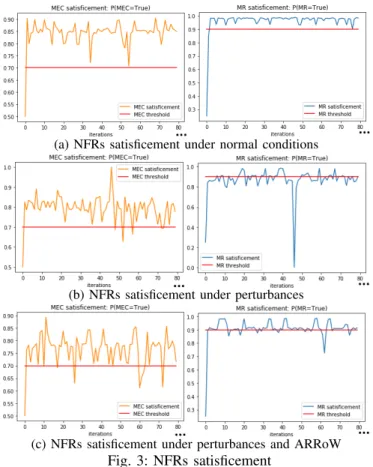
(e.g. Table I). A maximum deviation of 10 percent of the current transition function P(s’|s,a) has been performed. Each deviation lasts between 5 and 15 time slices, and its duration was also randomly selected to therefore simulate real situation. In Fig. 3a, a sample pattern for the satisficement of the NFRs MEC and MR under the current parameters of the POMDP model, is shown, i.e. without any perturbation and by using the current reward values, transition and observation functions. It is observed, that under normal conditions the satisficement of MEC and MR is in general over the identified thresholds: P(MEC=true >=0.7) and P(MR=True>=0.9).
(a) NFRs satisficement under normal conditions
(b) NFRs satisficement under perturbances
(c) NFRs satisficement under perturbances and ARRoW Fig. 3: NFRs satisficement
A new sample pattern for the current satisficement of MEC and MR after randomly injecting disturbances on the environment is also shown in Fig. 3b. Under the new context, the current reward values R(s,a) (See Table III), were not suitable anymore, as the satisficement of MR is under its tolerance threshold. Therefore, the current reward values R(s,a) were reassessed at runtime to improve the selection of the adaptation action a∈Ain the POMDP model.
2) Experiment execution: Runtime reassessment of rewards R(s,a) in the POMDP model: We highlight the role of the runtime models in the Knowledge Base in terms of the MAPE-K loop architecture (See Fig. 2). During the scenarios, the thresholds identified for each NFR are monitored. If the satisficement of any NFR is detected below its threshold; the reassessment and possible update of rewards R(s,a) is carried out by the weights updater module included in the planning phase of the MAPE-K Loop. Examples of possible
implementations for the runtimeweights updater module are found in [27], [21], [20]. Specifically, we have used the ARRoW model (Automatic Runtime Reappraisal of Weights) [20], that complements the POMDP model in the knowledge base of the MAPE-K architecture. The ARRoW model and the POMDP model constitutes the runtime K models (See Fig. 2). After this, the updated reward values constituteadditional inputfor theaction plannermodule, which continue with the process to select the best adaptation actiona∈A.
Fig. 3c shows a sampled pattern of the new satisficement for the NFRs MEC and MR after updating the reward values R(s,a). It is observed that the satisficement of MR is improved as a result of better informed decision-making provided by the POMDP model and the partially-observed values. A slight reduction on the satisficement of MEC is also noticed in the context where the rewards R(s,a) are not updated.
3) Experiment summary: Figs. 4a and 4b show the average satisficement of MEC and MR after 5 rounds during the first 1000 time slices each. The legend describes that in a round [round-n], na indicates that ARRoW is not used, and A indicates that ARRoW is used to update weights at runtime.
(a) Average satisficement for MR
(b) Average satisficement for MP Fig. 4: NFRs average satisficement
The results in Fig. 4a indicate that in each round, when the weights are not updated by ARRoW (See Fig. 4a, columns [round-n] na), the average satisficement level of MR is below its threshold, i.e. it is within a poor zone of satisficement due to unmatching initial rewards R(s,a) in the new environmental context (See Table III), while MEC is always within a suitable zone of satisficement (See Fig. 4b, columns [round-n] na). On the other hand, when updating weights using ARRoW (See Fig. 4a, columns [round-n] A), the satisficement level of MR was improved by leveraging access to new evidence. In exchange, a reduction in the satisficement level of MEC is
observed, however it is still within the suitable zone (See Fig. 4b, columns [round-n] A). Further experiments confirm the results above and show that updating the rewards R(s,a) the performance of the SAS is improved. Based on these findings, the proposed hypothesis H can be accepted as valid.
VI. RELATEDWORK
Different approaches exist that deal with uncertainty due to unpredictable changing environments [30]. REDAPT [30] is a method for mitigating runtime uncertainty for SAS by the specification of dynamic properties of an Adaptive Goal Model (AGM). Adaptation mechanisms are derived and adap-tations are achieved by diagnosing requirements violations to determine reconfigurations. As we do, they focus on the uncertainty on the satisficement levels of NFRs at runtime. However, while they use MAPE-K loops to refine NFR goals at runtime, they do not use learning. The authors in [8] assume that the impact of the adaptation actions on NFRs is deterministic. In contrast, we assume that the impact of actions on NFRs is uncertain and can change over time. The authors in [7], [19], [18] use a restricted version of POMDPs: Markov Decision Processes (MDPs) or Discrete Time Markov Chains (DTMC), where the knowledge of the state of the system is assumed in advance. In our case the state of the system is partially observable. We model it by updating the belief, i.e. the probability distributions, which can be based on monitored data as offered by the POMDP. In [12], Filieri et. al. showcase a mathematical framework for runtime model checking. Using a probabilistic Markov model at design time, verification conditions for requirements violations are defined. At runtime, these are evaluated according to changes in the environment. Non of the related work shown work with explicit runtime representations and its causal connection.
VII. CONCLUDINGREMARKS
Our work uses new evidence found at runtime to (i) pro-vide extra information during decision-making and, (ii) find opportunities to improve the SLA conformance by updating the rewards associated with NFRs and adaptation actions. As future work, we aim to exploit the potential for modularity of the architecture proposed by adding other runtime K models such as goal models [4]. Further, Bayesian learning offers a great potential for self-explanation [14]. Our target is to ex-plain to stakeholders of the system reasons why a reassessment of weights was applied, or a decision was made based on the support of POMDPs.
REFERENCES
[1] A. RAMIREZ, A. J.,ANDCHENG, B. a taxonomy of uncertainty for dynamically adaptive system,. Software Engineering for Adaptive and Self-Managing Systems (SEAMS), 2012 ICSE Workshop.(2012). [2] BAI, H., CAI, S., YE, N., HSU, D.,ANDSUN, W. Intention-aware
online pomdp planning for autonomous driving in a crowd. In Proc. IEEE Int. Conf. on Robotics & Automation(2015).
[3] BENCOMO, N., BENNACEUR, A., GRACE, P., BLAIR, G., ANDIS
-SARNY, V. The role of [email protected] in supporting on-the-fly interoperability.Computing 95, 3 (2012), 167–190.
[4] BENCOMO, N., GOTZ, S.,ANDSONG, H. [email protected]: a guided tour of the state-of-the-art and research challenges.Journal of Software and Systems Modeling (SoSyM)(2019).
[5] BENNACEUR, A., MCCORMICK, C., GARC´IA-GALAN´ , J., PERERA, C., SMITH, A., ZISMAN, A.,ANDNUSEIBEH, B. Feed me, feed me: an exemplar for engineering adaptive software. InSEAMS(2016). [6] BLAIR, G., BENCOMO, N.,ANDFRANCE, R. Guest editor’s
introduc-tion: [email protected]. IEEE Software(2009).
[7] CALINESCU, R., GRUNSKE, L., KWIATKOWSKA, M., MIRANDOLA, R., ANDTAMBURRELLI, G. Dynamic QoS management and opti-misation in service-based systems. IEEE Transactions on Software Engineering 37, 3 (2011), 387–409.
[8] C ´AMARA, J., PENG, W., GARLAN, D.,ANDSCHMERL, B. R. Reason-ing about sensReason-ing uncertainty and its reduction in decision-makReason-ing for self-adaptation. Sci. Comput. Program. 167(2018), 51–69.
[9] CHENG, B. H.,AND ET AL. Software engineering for self-adaptive systems. Springer-Verlag, Berlin, Heidelberg, 2009, ch. Software Engi-neering for Self-Adaptive Systems: A Research Roadmap, pp. 1–26. [10] DELEMOS, R., GIESE, H., M ¨ULLER, H.,ANDSHAW, M. Software
Engineering for Self-Adpaptive Systems: A second Research Roadmap. InSoftware Engineering for Self-Adaptive Systems(Germany, 2011). [11] ESFAHANI, N.,ANDMALEK, S. Uncertainty in self-adaptive software
systems. InSoftware Engineering for Self-Adaptive Systems 2 (SEfSAS 2). Springer-Verlag, 2012.
[12] FILIERI, A., TAMBURRELLI, G.,ANDGHEZZI, C. Supporting self-adaptation via quantitativeverification and sensitivity analysis at run time. IEEE TRANSACTIONS ON SOFTWARE ENGINEERING(2016). [13] FREDERICKS, E. M. Mitigating uncertainty at design time and run time to addressassurance for dynamically adaptive systems. Michigan State University. PhD Thesis.(2015).
[14] GARCIA-DOMINGUEZ, A., BENCOMO, N.,ANDGARCIAPAUCAR, L. Reflecting on the past and the present with temporal graph-based models.
MRT 2018. Copenhagen, Denmark, 14.-19. October 2018(2018). [15] GARCIA-PAUCAR, L., ANDBENCOMO, N. Re-storm: Mapping the
decision-making problem and non-functional requirements trade-off to partially observable markov decision processes. InSEAMS(2018). [16] JI, M., VEITCH, A. C., WILKES, J.,ET AL. Seneca: remote mirroring
done write. InUSENIX Annual Conference(2003), pp. 253–268. [17] KURNIAWATI, H., AND YADAV, V. An online pomdp solver for
uncertainty planning in dynamic environment. Proc. Int. Symp. on Robotics Research(2013).
[18] KWIATKOWSKA, M., NORMAN, G.,ANDPARKER, D. Probabilistic model checking: Advances and applications. InFormal System Verifi-cation(2017), Springer, pp. 73–121.
[19] MORENO, G. A., C ´AMARA, J., GARLAN, D.,ANDKLEIN, M. Uncer-tainty reduction in self-adaptive systems. InSEAMS(2018).
[20] PAUCAR, L. H. G., BENCOMO, N.,ANDFUNGYUEN, K. K. Juggling Preferences in a World of Uncertainty. RE NEXT, Lisbon.(2017). [21] PENG, X., CHEN, B., YU, Y.,ANDZHAO, W. Self-tuning of software
systems through goal-based feedback loop control. In Requirements Engineering Conference (RE)(Sept 2010), pp. 104–107.
[22] RAMIREZ, A., CHENG, B., BENCOMO, N.,ANDSAWYER, P. Relaxing claims: Coping with uncertainty while evaluating assumptions at run time. MODELS(2012).
[23] ROSS, S., PINEAU, J., PAQUET, S.,AND CHAIB-DRAA, B. Online planning algorithms for pomdps. J. Artificial Intelligence Research, 32(1), 663704(2008).
[24] RUSSELL, S. J.,ANDNORVIG, P. Artificial intelligence - a modern approach: the intelligent agent book. Prentice Hall series in artificial intelligence. Prentice Hall, 1995.
[25] RUTTEN, E., MARCHAND, N.,ANDSIMON, D. Feedback control as mape-k loop in autonomic computing. 349–373.
[26] SOMANI, A., YE, N., HSU, D.,AND LEE, W. S. Despot: Online pomdp planning with regularization. InAdvances in neural information processing systems(2013), pp. 1772–1780.
[27] SOUSA, J. P., BALAN, R. K., POLADIAN, V., GARLAN, D., AND
SATYANARAYANAN, M. User guidance of resource-adaptive systems. InIn Proc. of Intrl. Conf. on Software and Data Technologies(2008). [28] TARJAN, R. Depth-first search and linear graph algorithms.12th Annual
Symposium on Switching and Automata Theory.(1971).
[29] WALSH, W. E., TESAURO, G., KEPHART, J. O.,ANDDAS, R. Utility functions in autonomic systems. InAutonomic Computing(2004). [30] YANG, Z., ZHANG, W., ZHAO, H.,ANDJIN, Z. Requirements-driven
dynamic adaptation to mitigate runtime uncertainties for self-adaptive systems. CoRR abs/1704.00419(2017).
[31] YE, N., SOMANI, A., HSU, D.,ANDLEE, W. S. Despot: Online pomdp planning with regularization. J. Artificial Intelligence Research(2017).