A unified theory of empirical likelihood ratio confidence
intervals for survey data with unequal probabilities and
non negligible sampling fractions
Y.G. Berger and O. De La Riva Torres University of Southampton, UK
Summary. We propose a new empirical likelihood approach which can be used to construct design-based confidence intervals under unequal probability sampling without replacement. The proposed empirical likelihood confidence interval has the following advantages. It gives confidence intervals which may perform better than standard confidence intervals based on the central limit theorem. It does not rely on variance estimates, design effects or joint-inclusion probabilities. It can be applied to the Horvitz-Thompson estimator, the H ´ajek estimator or the regression estimator. It can be also used with large sampling fractions. The proposed approach also offers a unified likelihood-based justification for design-based approaches, such as calibra-tion, used in sample surveys.
Keywords: Calibration, Design-based approach, Finite population corrections, H ´ajek estimator, Horvitz-Thompson estimator, Regression estimator, Stratification, Unequal inclusion probabili-ties.
1. Introduction
Let U be a finite population of N units. Let yi and xi be, respectively, the values of the variable of interest and the vector of auxiliary variables attached to unit i. Note that N is a fixed quantity which is not necessarily known. Suppose that we want to estimate the population total Y =P
i∈Uyi. Suppose that a sample sof size nis selected with unequal probabilities without replacement with a sampling fractionn/N which can be large. Letπi denote the inclusion probability of uniti. LetPni=1 denote the sum over the sampled units. The totalY can be estimated by the Horvitz and Thompson (1952) estimator
b YHT = n X i=1 yi πi, (1)
by the H´ajek (1971) ratio estimator
b YH= PnN i=1π −1 i n X i=1 yi πi,
by regression estimators (e.g. Hartley and Rao, 1968; S¨arndalet al., 1992) or by empirical likelihood estimators. We consider a design-based approach; where the sampling distribution is specified by the sampling design.
Address for correspondence: Y.G. Berger, University of Southampton, Southampton Statistical Sciences Research Institute, Southampton, SO17 1BJ, UK. E-mail: [email protected]
One of the first attempts to formulate a likelihood-based approach is survey sampling is due to Godambe (1966) who showed that under the design-based approach, the standard likelihood function is flat and cannot be used for inference. A solution to this problem is to assume that the data is generated from a super-population model which can be used to derive a likelihood function (e.g. Cassel et al., 1977, Ch. 4). However this approach relies on super-population models which are not always suitable for the production of survey estimates. Hartley and Rao (1968) introduced the empirical likelihood approach under the name of scale load approach which provides a likelihood-based approach which does not relies on models. Owen (1988) brought this approach into the mainstream statistics (see also Owen, 2001). Since Chen and Qin (1993) suggested its first application in survey sampling, there have been many recent developments of empirical likelihood based methods in survey sampling (e.g. Rao and Wu, 2009) and adaptive sampling (Salehiet al., 2010). However, the traditional empirical likelihood approaches (Rao and Wu, 2009) are not entirely satisfactory and have several disadvantages described below. The proposed empirical likelihood approach does not have these disadvantages and can be implemented with a larger class of sampling designs and estimators.
Standard confidence intervals based upon the central limit theorem can perform poorly when the sampling distribution is not normal. For example, the lower bounds of a confidence interval can be negative even when the parameter of interest is positive. The coverage and the tail errors can be also lower than their intended levels. On the other hand, empirical likelihood confidence intervals (Owen, 2001) may be better in this situation, as empirical likelihood confidence intervals are determined by the distribution of the data (Rao and Wu, 2009) and the range of the parameter space is preserved.
Chen and Sitter (1999) proposed a pseudo empirical likelihood approach which can be used to construct confidence intervals (Wu and Rao, 2006). The pseudo empirical likelihood approach is not entirely appealing from a theoretical point of view, as it is not applicable to the Horvitz and Thompson (1952) estimator and it relies on variance estimates (Rao and Wu, 2009). This approach consists in maximising the pseudo empirical likelihood function under a set of constraints. Confidence intervals are computed using an empirical log-likelihood ratio function multiplied by a design effect which takes into account of the sampling design. This approach is not a genuine empirical likelihood approach (Rao and Wu, 2009), as confidence intervals rely on variance estimates or design effects which can difficult to compute when, for example, the joint inclusion probabilities are unknown. The proposed approach does not rely on variance estimates, design effects or joint inclusion probabilities, as it will not be necessary to multiply the empirical log-likelihood ratio function by a design effect.
The pseudo empirical likelihood approach cannot be used to derive a confidence interval for the Horvitz and Thompson (1952) estimator YbHT. However it can be used to derive confidence intervals for the H´ajek (1971) estimator YbH. When yi is highly correlated with πi, we prefer to use the more efficient estimator YHTb rather than YHb (Rao, 1966). For example, with business surveys, it is common to have a strong correlation; and YHb would be a poor estimator in this case. In this situation, the pseudo empirical likelihood approach gives a confidence interval for the less efficient estimator, YHb . The proposed approach is more flexible, as confidence intervals forYHTb orYHb can be computed.
In this paper, we propose to use a new empirical likelihood approach which is differ-ent from the pseudo empirical likelihood approach. We show that the empirical likelihood function considered is a genuine empirical likelihood function. We show that the Horvitz and Thompson (1952) estimator is the maximum likelihood estimator when we do not use
auxiliary variables. When we include a calibration constraint on the auxiliary variables (e.g. Huang and Fuller, 1978; Deville and S¨arndal, 1992), the maximum likelihood estimator is asymptotically equivalent to the regression estimator (e.g. Hartley and Rao, 1968; S¨arndal
et al., 1992).
The main contribution of this paper is to show that under a series of regularity conditions, the proposed empirical log-likelihood ratio function converges to a chi-squared distribution with one degree of freedom without the need of adjusting the empirical log-likelihood ratio function by a design effect. This property depends on a set of constraints which takes account of the sampling design and the auxiliary variables. We show this property can be used to derive confidence intervals for the Horvitz and Thompson (1952) estimator, the H´ajek (1971) estimator and the regression estimator, when the sampling fraction is large or negligible.
When deriving asymptotic results associated with the empirical likelihood based method, it is common practice to assume that the sampling fraction is negligible (n/N → 0) (e.g. Wu and Rao, 2006, p. 364, Zhong and Rao, 2000, p. 933, Rao and Wu, 2009, p. 192). This assumption limits the applicability of these methods, as many surveys use sampling fractions which are not necessarily negligible. For example, with business surveys, it is common practice to have large sampling fractions. Note that empirical likelihood confidence intervals have better coverage than standard confidence intervals when the variable of interest is very skewed or contains many zeros (Chenet al., 2003) which is a common situation with business surveys or when we are interested in domains’ totals. The proposed empirical likelihood approach does not rely on the assumption n/N →0, and can be used when the sampling fraction is large.
In §2, we define the class of sampling designs considered. In §3, we define the proposed empirical likelihood function and in§4, we show how the parameters of the empirical like-lihood function can be estimated. In §5, we define the empirical likelihood estimators of a total. The asymptotic framework and the regularity conditions are given in §6. In §7, we show that these estimators reduce to the Horvitz and Thompson (1952) estimator, the H´ajek (1971) estimator or the regression estimator (e.g. Hartley and Rao, 1968; S¨arndal
et al., 1992) depending on the constraints considered. In §8, we define the proposed empir-ical log-likelihood ratio function, and in §9 show how this function can be used to derive non-parametric confidence intervals. In §10, we show that the sampling distribution of the proposed empirical log-likelihood ratio function converges to a chi-squared distribution. In §11, we show via a series of simulations that the proposed empirical likelihood approach gives confidence intervals which perform better than standard confidence intervals.
2. Stratified unequal probability sampling
Assume that the samplesis randomly selected by a uni-stage stratified probability sampling designp(s). Suppose that the finite populationU is stratified intoH strata denoted byU1, U2, . . ., UH; where ∪Hh=1Uh = U. The size of Uh is denoted by Nh with
PH
h=1Nh = N. Suppose that a sample sh of fixed size nh is selected without replacement with unequal probabilitiesπi fromUh. The complete sample is given bys=∪h=1H sh. Letn= (n1, . . . nH)0 denote the vector of the strata sample sizes. The sampling design depends on design variables which contains the information about the stratification and the inclusion probabilities. The design variables have the following values attached to uniti.
where zih =πi δ{i ∈Uh}. The function δ{A} is the Dirac measure which is equal to one whenAis true and zero otherwise. Note that because a fixed size sample is selected within each stratum, we have the following fixed sizes constraint.
n X i=1 zi πi = X i∈U zi=n· (2)
We suppose that the sample is selected according to a high entropy stratified sampling design with unequal probabilities (e.g. H´ajek, 1981; Berger, 1998; Brewer and Donadio, 2003; Till´e, 2006; Berger, 2011). For example the Rao-Sampford (Rao, 1965; Sampford, 1967) and the Chao (1982) sampling designs are high entropy sampling designs (Berger, 2005, 2011). Note that most sampling designs used in practice have large entropy, except the non-randomized systematic sampling design. The maximum entropy sampling design is the conditional Poisson sampling design (H´ajek, 1981). Berger (2011) showed that the high entropy sampling designs and the conditional Poisson sampling design are asymptotically equivalent.
The conditional Poisson sampling design (H´ajek, 1981; Fuller, 2009) can be implemented by using a rejective approach (H´ajek, 1964) which consists in selecting several Poisson samples with inclusion probabilitiesπiand retaining the first sample which is such that the fixed sizes constraint (2) holds. Note that the final sample retained is not Poisson samples because the sample sizes are fixed and given by n. Note that the conditional Poisson sampling design can also be implemented by selecting a rejective sample within each stratum. Note that the inclusion probabilities are not exactly given by πi, because of the rejective nature of this sampling design. However, H´ajek (1964) showed that (1) is asymptotically equivalent to the Horvitz and Thompson (1952) estimator with the correct inclusion probabilities.
3. Empirical likelihood function under unequal probability sampling
Let {y1, . . . , yn} denote a set of n independent and identically distributed observed values from a distributionF. The distribution function that has support on this set is given by
Fm(x) = n X i=1 [F(yi)−F(yi−)]δ{i≤x}= Pn i=1mi δ{i≤x} Pn i=1mi ; (3)
where the quantitymi is proportional to the mass of uniti in the population (e.g. Deville, 1999); that is,mi∝[F(yi)−F(yi−)]; whereF(y
−
i ) =limy↑yiF(yi).
The distribution function (3) is valid if the observations are independent and identically distributed. However, this is not the case when the sample is selected with an unequal probability sampling design. Hence, we need another distribution function which is different from (3) and which takes the sampling design into account. Consider that the set of observed values is selected according to a fixed size conditional Poisson sampling design. In Appendix A, we show that the sample distribution under conditional Poisson sampling is given by
Fs(x) = Pn
i=1πi mi δ{i≤x} Pn
j=1πj mj
· (4)
Theempirical likelihood functionis defined by (see Owen, 2001, p. 7) L(m) =
n Y i=1
Hence using (4), we have the following empirical likelihood function. L(m) = n Y i=1 πi mi Pn j=1πj mj ! · (5)
Note that Kim (2009) proposed a similar empirical likelihood function under Poisson sampling and with probability mass instead of the massmi. Kim (2009) did not show how this function can be used to contruct confidence intervals.
When the sampling design is different from the conditional Poisson sampling design, we propose to use the same empirical likelihood given by (5). We will show that the empirical log-likelihood ratio function (see§8) gives correct confidence intervals even when the sampling design is different from the conditional Poisson sampling design, as long as the entropy is large, because the empirical log-likelihood ratio function has the same sampling distribution under Poisson sampling or under large entropy sampling (Berger, 2011).
4. Maximum empirical likelihood estimator of the mass measure
The maximum likelihood estimators ofmiare the valuesmbiwhich maximise thelog-empirical
likelihood function
`(m) = log(L(m)), (6)
subject to the constraintsmi≥0 and n X i=1
mici = C; (7)
where ci is a knownQ×1 vector associated with the i-th sampled unit and C is a known Q×1 vector. Note that the vectorC is not necessarily a vector of fixed quantities. HenceC
can be fixed or random. Possible choices forci andC are discussed in§10. The constraint (7) resembles the constraint used in calibration (e.g. Huang and Fuller, 1978; Deville and S¨arndal, 1992). However, we will see in §10 that C is not necessarily a vector of population totals of auxiliary variables.
We can find a solution to this minimisation problem using the Lagrange multipliers method which consists in minimising the following function.
Q(m,λ) = n X i=1
log(πi mi)−nlog n X i=1 πi mi ! − n Nλ 0 n X i=1 mici−C ! ·
The values of mi and λ which minimise Q(m,λ) are the solutions of the following set of equations∂Q(m,λ)/∂mi= 0 and ∂Q(m,λ)/∂λ= 0. The solution is
b mi= 1 n π i nκ+ 1 Nλ 0c i −1 , (8) where κ= 1 n n X j=1 πj mj· (9)
The parameters κand λ are such that the constraint (7) holds. The parameters κand λ
4.1. Iterative Newton-Raphson procedure Let f(κ,λ) = 1 N n X i=1 b mici·
Note thatf(κ,λ) is aQ×1 vector function ofκandλ, because thembi depend onκandλ. Suppose thatκis a given quantity. A Taylor approximation off(κ,λ) in the neighbour-hood of an initial guessλ0is given by
f(κ,λ)−f(κ,λ0)l∆(b κ,λ0) (λ−λ0), (10) where∆(b κ,λ) is the followingQ×Qgradient matrix.
b ∆(κ,λ) =∂f(κ,λ) ∂λ =− 1 nN2 n X i=1 cic0i πi κn+ 1 Nλ 0c i −2 · (11)
As the constraint (7) can be re-written as f(κ,λ) = CN−1, we have that λ l λ0 − b
∆(κ,λ0)−1(f(κ,λ0)−CN−1), using (10). Hence, the following recursive formula can be used to computeλ,
λ`+1=λ`−∆(b κ,λ`)−1(f(κ,λ`)−CN−1)· (12)
We propose to calculateλiteratively with λ0=0andκ= 1. The solution of (12) gives a new set of weightsmib which substituted into (9) gives a new value forκwhich gives a new value forλby using (12). We repeat this process several times until convergence. Note that κis generally very close to one.
5. Maximum empirical likelihood estimator of a total
Themaximum empirical likelihood estimator of a total is defined by the following function of the maximum empirical likelihood estimators of the mass measure.
b τ = n X i=1 b miyi, (13)
where mib is defined by (8). An alternative estimator is the following maximum empirical likelihood ratio estimator of a total.
b τr=N Pn i=1mbiyi Pn i=1mib · (14)
Note that both estimators depend on the values ofci andC and that themib play the role of survey weights.
Note that when ci =zi and C =n, we have thatλ=0, κ= 1 and mib =π −1
i . In this case, (13) reduces to the Horvitz and Thompson (1952) estimatorYHTb and (14) reduces to the H´ajek (1971) ratio estimator YHb . The estimator YHTb is more efficient than YHb when the variable of interest is correlated with the inclusion probabilities (Rao, 1966). When the variable of interest and the inclusion probabilities are not correlated,YbHT can be less efficient
thanYHb (Rao, 1966). In this situation , we suggest using (14) which reduces to the H´ajek (1971) ratio estimator whenci=zi andC =n.
Wu and Rao (2006) proposed to use the pseudo empirical likelihood estimator with zi treated as values of auxiliary variables. This gives a pseudo empirical likelihood estimator which is different fromYbHT andYbH. Note that with the pseudo-empirical likelihood approach (Chen and Sitter, 1999), it is not possible to obtain the Horvitz and Thompson (1952) estimatorYbHT.
6. Asymptotic framework
In order to derive asymptotic properties of the proposed empirical likelihood approach, it is necessary to define the asymptotic framework and a set of regularity conditions.
We use the H´ajek (1964) asymptotic framework. Consider a sequence of stratified samples stselected from the sequence of nested finite populationsUtwith a stratified sampling design p(s)twith inclusion probabilitiesπt
iwheret= 1, 2, . . .. All limiting processes are understood to be as t → ∞. In what follows, a constant will be a scalar free of t. For simplicity of notation, the indextis suppressed in what follows.
We assume that
dh= X i∈Uh
πi(1−πi)→ ∞, (15)
for all h and that the number of strata H is bounded (H = O(1)). The stochastic order O(·), o(·), Op(·) and op(·) are defined according to this asymptotic framework, where the convergence in probability is with respect to the sampling design. The assumption (15) was first suggested by H´ajek (1964). This assumption implies that nh → ∞ and Nh → ∞, as dh < nh < Nh. We also assume that nh/Nh → fh, where fh is a positive constant. Berger (2011) showed that under these assumptions and other mild regularity conditions, high entropy sampling designs and the conditional Poisson sampling design are asymptotically equal.
Consider the following regularity conditions.
N−1kCbπ−Ck = Op(n−ψ), (16) nN−1max{πi−1kcik:i∈s} = op(n1/2), (17) nN−1max{πi−1|yi|:i∈s} = op(n1/2), (18) kbSk = Op(1), (19) kbS−1k = Op(n2ψ−1), (20) 1 nNτ n X i=1 kcikτ πτ i = Op(n−τ), (21) 1−κ = Op(n−µ), (22) withψ >1/2,τ≤3,µ >1/2, b S = ∆(b κ,0), b Cπ = n X i=1 ci πi, (23)
where∆(b κ,0) is given by (11) with λ=0. The quantitykAk= trace(A0A)1/2denotes the Euclidean norm
Isaki and Fuller (1982) gave conditions under which (16) holds. Under the condition nN−1π−1
i = Op(1) proposed by Krewski and Rao (1981, p. 1014), the conditions (17) and (18) hold when (i) max{|yi| : i ∈ s} = op(n1/2) and when (ii) max{kcik : i ∈ s} = op(n1/2). Chen and Sitter (1999, Appendix 2) showed that the conditions (i) and (ii) hold for common unequal probability sampling designs. The matrix Sb is equal to a covariance matrix between totals multiplied by−κ2n/N2. Thus the condition (19) holds when the norm of this covariance matrix variance decreases with raten−1. The condition (20) means that kSbkis bounded away for a quantity or orderOp(n1−2ψ). The condition (21) is a Lyapunov-type condition for the existence of moments. The condition (22) holds asκis close or equal to one.
Note that using (17) and Lemma 3 (in Appendix B), we have thatmbiπi =Op(1) which implies that we have a negligible probability to havembi a lot larger thanπi−1.
7. Approximation of the maximum empirical likelihood estimator of a total
The following lemma will be useful to derive an approximation of the maximum empirical likelihood estimator of a total and to derive the asymptotic distribution of the empirical log-likelihood ratio function in§10.
Lemma 1. Letλbe the solution of (7) for givenciandC. Under the regularity conditions
(16)-(22), we have that
λ=N−1Sb −1
(C−Cbπ) +be, (24)
wherekbek=op(n−1/2) andCbπ is defined by (23).
The proof of Lemma 1 is given in Appendix B.
In Appendix C, we show that the Lemma 1 implies that the maximum empirical likelihood estimator (13) is asymptotically equivalent to
b
τ = YHTb +Bb 0
(C−Cbπ) +op(N), (25)
under the regularity conditions (16)-(22), whereBb is a vector of regression coefficients defined by b B = n X i=1 1 π2 i cic0i !−1 n X i=1 1 π2 i yici· (26)
Note that when ci is a vector of auxiliary variables and C is the associated vector of population totals, (25) is the generalised regression estimator (e.g. S¨arndal et al., 1992, p. 228). When ci = (x0i,z0i)0 and C =
P
i∈Uci, (25) is the generalised optimal regression estimator (e.g. Isaki and Fuller, 1982; S¨arndal, 1996; Bergeret al., 2003).
Note that there is a clear analogy between the proposed empirical likelihood approach and calibration (e.g. Huang and Fuller, 1978; Deville and S¨arndal, 1992), as the function (6) can be viewed as a calibration distance function, and the empirical likelihood estimator is asymptotically equivalent to a calibrated regression estimator (25).
8. Empirical log-likelihood ratio function
Let mib be the values which maximise (6) subject to the constraints mi ≥ 0 and (7) for given values for ci and C. Let `(mb) be the maximum value of (6). Let mb
∗
i be the values which maximise (6) subject to the constraintsmi≥0 and (7) with ci =c∗i = (c0i, yi∗)0 and
C =C∗ = (C0, y∗)0. In §10, we give examples of values for y∗i and y∗. Let `(mb∗) be the maximum value of (6). Theempirical log-likelihood ratio function is defined by the following function ofy∗
b
r(y∗) = 2{`(mb)−`(mb∗)} · (27) Note that for a given value ofy∗, the quantitybr(y∗) is a random variable with a distribution specified by the sampling design.
9. Empirical likelihood confidence intervals
The main advantage of empirical likelihood approach is its capability of deriving non-parametric confidence intervals which do not depend on variance estimates. In §10, we show that the sampling distribution of the empirical log-likelihood ratio function is such that P rbr(Y)≤χ21(α) l1−α, (28) whereY denotes the population total andP r{·}denotes the probability with respect to the sampling design. The quantityχ21(α) is the upperα-quantile of the chi-squared distribution with one degree of freedom. In §10, we show that the property (28) holds for the Horvitz and Thompson (1952) estimator, the H´ajek (1971) estimator and the regression estimator (e.g. Hartley and Rao, 1968; S¨arndal et al., 1992) when the sampling fraction is large or negligible. We will see that (28) holds even if the sampling design is different from the conditional Poisson sampling design.
As the property (28) holds, the (1−α) level empirical likelihood confidence interval (e.g. Wilks, 1938; Hudson, 1971) for the population totalY is given by
min
y|rb(y)≤χ21(α) ; max
y|br(y)≤χ21(α) ·
Note that br(y) is a convex non-symmetric function with a minimum when y is the max-imum empirical likelihood estimator. This interval can be found using a bijection search method within the interval [Nmin{yi|i∈s}, Nmax{yi|i∈s}] (e.g. Wu, 2005). This involves calculatingbr(y) for different values of y.
Standard confidence intervals based upon the central limit theorem can perform poorly when the sampling distribution is not normal (Wu and Rao, 2006). On the other hand, em-pirical likelihood confidence intervals may be better in this situation, as emem-pirical likelihood confidence intervals are determined by the distribution of the data (Rao and Wu, 2009) and the range of the parameter space is preserved (Wu and Rao, 2006). This may not be the case for standard confidence intervals, as they can have negative lower bounds even when the parameter of interest is positive. In§11, we show via a series of simulation that the proposed empirical likelihood approach gives confidence intervals which perform better than standard confidence intervals.
10. Asymptotic distribution of the empirical log-likelihood ratio function
In this §, we show that the property (28) holds for the Horvitz and Thompson (1952) esti-mator, the H´ajek (1971) estimator and the regression estimator (e.g. Hartley and Rao, 1968; S¨arndalet al., 1992) when the sampling fraction is large or negligible. This result relies on the following assumption.
P rn(Yb −Y)2var[Yb]−1≤χ21(α) o
l1−α, (29)
where Yb is an estimator of the total Y, var[Yb] is the design-based variance of Yb. Note that the assumption (29) holds when Yb is asymptotically normally distributed. However the assumption (29) is weaker that asymptotic normality, as (29) may hold even when Yb is not normally distributed. Note the assumption of asymptotic normality is usually made, when showing that the empirical log-likelihood ratio function converges to a chi-squared distribution (e.g. Owen, 2001, p. 219, Wu and Rao, 2006, p. 364).
Using the following Lemma, we can derive the approximation (32) of the empirical log-likelihood ratio function.
Lemma 2. Letλthe solution of (7) for givenci andC. Under the regularity conditions
(16)-(22), we have that `(mb) +nlog(n) = −1 2 (Cbπ−C) 0 b Σ−1(Cbπ−C) +op(1), (30)
whereCbπ is defined by (23) and Σb =−N2n−1κ−2S.b
The proof of Lemma 2 is given in Appendix D. Lemma 2 implies that
`(mb∗) +nlog(n) =−1 2 (Cb ∗ π−C ∗)0 b Σ∗−1(Cb ∗ π−C ∗) +o p(1), (31) whereCb ∗ π = Pn i=1c∗iπ−1i andΣb ∗ =−N2n−1κ∗−2 b S∗, where Sb ∗ is given by (11) with λ=0, κ=κ∗,ci=c∗i andC =C
∗. Note that the matrix b Σ∗ can be re-written as b Σ∗= n X i=1 1 π2 i c∗ic∗i0 = Σb ∗ cc Σb ∗ cy b Σ∗ 0 cy σb ∗ yy ! where b Σ∗cc= n X i=1 1 π2 i cic0i=Σb, Σb ∗ cy = n X i=1 1 π2 i ciyi∗, σb∗yy= n X i=1 yi∗2 π2 i ·
By taking the difference between equations (30) and (31), we have that
b r(y∗) = (Cb ∗ π−C ∗)0 b Σ∗−1(Cb ∗ π−C ∗)−( b Cπ−C)0Σb −1 (Cbπ−C) +op(1)· (32)
10.1. Empirical likelihood approach for negligible sampling fractions
Letci=zi,C =Z=Pi∈Uzi andyi∗=yi. It can be shown thatmbi= 1/πi andbτ=YbHT is the Horvitz and Thompson (1952) estimator (1). Because of the fixed sizes constraint (2), we have thatCbπ−C=0H andCb
∗ π−C
∗= (00
H,YbHT−y∗)0, where0H is aH×1 vector of zeros. Thus (32) reduces to
b r(y∗) = (00H,YHTb −y∗)Σb ∗−1 (00H,YHTb −y∗)0+op(1) = (YHTb −y∗) 2 (bσyy∗ −Σb ∗0 cyΣb ∗−1 cc Σb ∗ cy)−1+op(1)· (33) AsΣb ∗ cc=diag{n1, n2, . . . , nH} andΣb ∗ cy = (Yb (1) π ,Yb (2) π , . . . ,Yb (H)
π )0, it can be shown that
b σyy∗ −Σb ∗0 cyΣb ∗−1 cc Σb ∗ cy =dvarpps[YHTb ],
where vardpps[YbHT] is the following pps stratified variance estimator (e.g. Durbin, 1953; S¨arndalet al., 1992, p. 99). d varpps[YbHT] = H X h=1 X i∈sh ˘ yi−n−1h Ybπ(h) 2 ,
where ˘yi=yi/πi. Therefore, asbτ=YHTb , we have thatdvarpps[τb] =dvarpps[YHTb ] and
b
r(y∗) = (bτ−y∗)2 dvarpps[τb]−1+op(1)·
When the sampling fractions are negligible,dvarpps[τb] is a consistent estimator for the variance (Durbin, 1953). Hence the assumption (29) implies the property (28) by Slutsky’s theorem. It can be shown that the property (28) holds for the maximum empirical likelihood ratio estimator (14) if we modify the values of yi∗ and y∗. Let yi∗ be the value of the linearised variable of a ratio estimator; that is, yi∗ = yi−N−1τrb (e.g. Deville, 1999). By usingy∗=y−YHTb , we have that
b
r(y) = (τbr−y)2 vardpps[bτr] −1+o
p(1),
treatingrb(y∗) as a function ofy, wherevarppsd [bτr] is the linearisedppsvariance estimator of (14) (e.g. S¨arndalet al., 1992, p. 178, Deville, 1999). Thus the property (28) holds for the maximum empirical likelihood ratio estimator.
10.2. Empirical likelihood approach for non negligible sampling fractions
In this case, the maximum empirical likelihood point estimator is still obtained usingci =zi andC=n; that isτb=YHTb .
In order for property (28) to hold, it is necessary to modify the ci and the yi∗ when computing the empirical log-likelihood ratio function. Let ci = qizi, yi∗ =qiyi, y∗ = y+ Pn i=1y ∗ iπ −1 i −YbHT and C = Pn
i=1ciπ−1i ; where qi = (1−πi)1/2. Note that for small sampling fractions,qil1 and we have the same ci,y∗i,y∗, C as in§10.1. It can be shown that mbi= 1/πi andτb=YbHT. We have thatCbπ−C =0
0 H andCb ∗ π−C ∗= (00 H,YbHT−y).
Hence (32) reduces to (33) with b Σ∗cc = n X i=1 (1−πi)ziz0iπi−2=diag{d1,b d2, . . . ,b dH},b b Σ∗cy = n X i=1 (1−πi)ziy˘iπ−1i = (Ye1, . . . , Yeh, . . . , YeH)0, b σ∗yy = n X i=1 (1−πi)˘yi2; wheredhb =Pi∈s h(1−πi) andYhe = P
i∈sh(1−πi)˘yi. It can be shown that
b σ∗yy−Σb ∗0 cyΣb ∗−1 cc Σb ∗ cy=vard[YHTb ], wherevard[Yb (h)
π ] is the following stratified H´ajek (1964, p. 1520) variance estimator
d var[YbHT] = H X h=1 " X i∈sh (1−πi)˘yi2−db−1h Yeh # · (34)
Therefore, asYbHT =bτ, we have that
b
r(y) = (τb−y)2vard[τb]−1+op(1), (35)
treatingbr(y∗) as a function ofy, where vard[bτ] =dvar[YHTb ].
The within stratum H´ajek (1964) variance estimator is consistent whendh→ ∞. Hence (34) is consistent because the number of strata is asymptotically bounded. Berger (2011) showed that this estimator is consistent under maximum entropy sampling. Thus, using assumption (29), we have that the property (28) holds by Slutsky’s theorem. Note that this result holds for large and small sampling fractions, and that the finite population correction are naturally included in (34).
With the maximum empirical likelihood ratio estimator, we need to use yi∗ = qi(yi − N−1bτr) andy∗=y+ Pn i=1y ∗ iπ −1
i −τbr. In this situation, it can be shown that the property (28) holds for the maximum empirical likelihood ratio estimator.
10.3. A restricted empirical likelihood approach for auxiliary variables
Letxibe aP vector of values of auxiliary variables associated with unit i. We assume that the vector of population totalsP
i∈Uxi is known. Letmbi(x) be the values which maximise (5) under the constraint (7) withci= (x0i,z0i)0 andC =
P
i∈Uci. The empirical likelihood estimator of a totalτb(x) =Pni=1mbi(x)yi(see (25)) is asymptotically equal to the generalised optimal regression estimator (Isaki and Fuller, 1982; S¨arndal, 1996; Bergeret al., 2003).
In order for the property (28) to hold, it is necessary to use the following restricted empirical likelihood function instead of the function (5) when calculating the empirical log-likelihood ratio function.
e L(mb) = n Y i=1 mi mib (x)−1 Pn j=1mj mjb (x) −1 ! · (36)
Note that (36) will be used for the calculation of the empirical log-likelihood ratio function, and not for the empirical likelihood point estimator. Note that the function (36) reduces to the function (5) when we do not have auxiliary variables. Because we use (36) instead of (5), the components of the matrix∆(b κ,λ) are given by (11), after substitutingπi bymbi(x)
−1. Let ci =qi(x0i,z0i)0, y∗i =qiyi, y∗ =y+ Pn i=1y ∗ imbi(x)−bτ(x), C = Pn i=1cimbi(x) and qi= (1−πi)1/2. Therestricted empirical log-likelihood ratio function is given by
e
r(y∗) = 2nlog(Le(mb))−log(Le(mb∗)) o
· (37)
It can be shown that er(y∗) is approximated by (32), where Cbπ = Pn
i=1ci mib (x) −1 and
C∗=Pni=1c∗i mbi(x)−1. It can be shown thatCbπ−C=0
0 H andCb ∗ π−C ∗= (00 H,τb(x)−y) 0. Hence (32) gives the following approximation.
e
r(y) = (bτ(x)−y)2vard[τb(x)]−1+op(1),
treatinger(y∗) as a function ofy. The quantityvard[bτ(x)] is an estimator of the variance of
b
τ(x). This variance takes into account of the calibration constraintPni=1mixi =Pi∈Uxi and of the fixed sizes constraint (2). Deville and Till´e (2005) gave an analytic expression of this estimator and showed that this estimator is approximately unbiased under fixed size sampling designs. Thus the property (28) holds with the function (37).
With auxiliary variables, the maximum empirical likelihood ratio estimator is given by
b τr(x) =N Pn i=1mib (x)yi Pn i=1mib (x) ·
In order for the property (28) to hold with the function (37), we need to use (36) with yi∗=qi(yi−N−1τbr(x)) andy ∗=y+Pn i=1y ∗ iπi−1−bτr(x). 11. Simulation study
We generated several population data according to the following model proposed by Wu and Rao (2006).
yi= 3 +ai+βxi+ϕ ei,
whereai andxi follow independent exponential distributions with rate parameters equal to one and ei ∼χ2
1−1. The πi are proportional to ai+ 2. The constant 2 is added toai to avoid having very smallπi. The parameterϕ is used to obtain a weak (0.30) and a strong correlation (0.80 or 0.75) between the valuesyi and ˆyi= 3 +ai+βxi. The parameterβ will be equal either to zero or one.
We use the Chao (1982) sampling design to select 1000 samples with unequal probabilities in order to compare the Monte-Carlo performance of the 95% empirical likelihood confidence interval with the standard confidence interval based on the central limit theorem. With this design, it is possible to compute the joint inclusion probabilities exactly and the Sen-Yates-Grundy variance estimator (Sen, 1953; Yates and Grundy, 1953) which is needed for standard confidence intervals. We consider that we have one stratum.
The coverages of the confidence intervals are reported in Tables 1, 2 and 3. As the 1000 samples are selected independently, we can use the de Moivre-Laplace theorem to test if the coverages are significantly different from 95% or if the tail error rates are significantly different from 2.5%. The symbols∗ and∗∗indicate significant differences (∗: 1%<p-value ≤5%;∗∗: p-value≤1%).
11.1. Empirical likelihood confidence intervals with small sampling fractions
For the first series of simulations, we generate population data of sizeN = 800 withβ = 0. The xi are not generated. Different sample sizes are considered: n = 40 and 80. As the sampling fractions are small, the approach described in§10.1 is used to derive the empirical likelihood confidence intervals. Consider ci = zi = (πi), C = Pi∈Uzi = (n) and yi∗ = yi. Note that in this case, the maximum empirical likelihood estimator is the Horvitz and Thompson (1952) estimator.
Table 1 gives the observed coverage probability, the lower and the upper tail error rates and the average length of the 95% confidence intervals. Note that the correlation is the cor-relation between the variable of interest and the inclusion probabilities. Note the confidence intervals computed with the proposed empirical likelihood approach perform better than the standard confidence interval, because the coverages are not significantly different from 95% and the lower and upper tail error rates are closer to 2.5%.
Table 1 can be compared with the results of the Wu and Rao (2006) simulation study, because the data was generated the same way. Wu and Rao (2006) used the pseudo empirical likelihood confidence intervals for the H´ajek (1971) estimatorYHb . In our series of simulations, we have the confidence interval for the Horvitz and Thompson (1952) estimatorYbHT. As far as the coverages are concerned, our results are similar to the results of Wu and Rao (2006). However, The average length of proposed empirical likelihood confidence intervals is smaller than the average length of the confidence interval of the H´ajek (1971) estimator obtained using pseudo empirical likelihood. This difference is more pronounced with large correlation, as in this case,YbHT is more accurate than YbH (Rao, 1966).
11.2. Empirical likelihood confidence intervals with large sampling fractions
For the second series of simulation, we generate population data of size N = 150 with β = 0. The xi are not generated. Different sample sizes are considered: n = 40 and 80. As the sampling fractions are large, the approach described in §10.2 is used. Note that the maximum empirical likelihood estimator is still the Horvitz and Thompson (1952) estimator. The observed coverages of the confidence intervals are given in Table 2. We see that for large sample sizes, the empirical likelihood confidence intervals have coverages and tail error rates which are not significantly different from 95% and 2.5%. On the other hand, the standard confidence intervals have poor coverages and tail error rates in all cases. For small sample sizes, the empirical likelihood confidence intervals have better lower tail error rates than the standard confidence intervals.
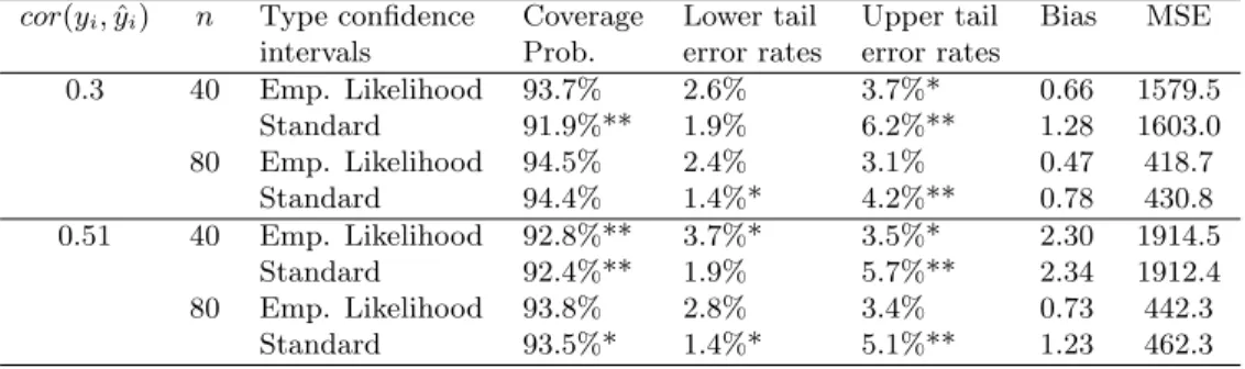
11.3. Restricted empirical likelihood confidence intervals with one auxiliary variable For the third series of simulation, we generate population data of sizeN = 150 withβ = 1. In this case, the values xi of the auxiliary variable are generated. A random set of 80% of the values of yi are replaced by zeros. Different sample sizes are considered: n = 40 and 80. The standard confidence interval is based on the standard regression estimator defined by (6.4.2) in S¨arndalet al.(1992). Note that this estimator is equal to the right hand side of (25) when ci =xi andC =Pi∈Uxi. The variance estimator of the standard regression estimator is given by (6.6.4) in S¨arndalet al.(1992).
The observed coverages of the confidence intervals and the mean square error of the point estimators are given in Table 3. We observe better coverages for the empirical likelihood confidence intervals except when the correlation is strong and the sample size is small. The
biases of the empirical likelihood estimator are slightly smaller, although none of the biases are significantly different from zero. It is not surprising to observe smaller mean square errors for the empirical likelihood estimator, because this estimator is asymptotically equivalent to the optimal regression estimator (see§7).
12. Discussion
The proposed empirical likelihood approach provides a likelihood-based justification of es-timators used in sample surveys, such as the Horvitz and Thompson (1952) estimator, the H´ajek (1971) estimator, the regression estimator (e.g. Hartley and Rao, 1968; S¨arndalet al., 1992) and calibration estimators (e.g. Huang and Fuller, 1978; Deville and S¨arndal, 1992), as we have shown that these estimators are maximum empirical likelihood estimators. The distance functions used in calibration are disconnected from mainstream statistical theory. However, the proposed distance function (6) is clearly related to the concept of likelihood. The proposed empirical likelihood function (6) has some advantages over some of the tradi-tional calibration distances. The ‘calibrated’ empirical likelihood weights are always positive and the empirical likelihood function can be used to construct likelihood ratio confidence intervals (e.g. Wilks, 1938; Hudson, 1971).
The proposed empirical likelihood approach can be easily generalised for multi-stage designs (e.g. S¨arndalet al., 1992§4.3.2), by substituting theyi by the first-stage totals. In this case, thezi specify the stratification used at the first-stage. The empirical log-likelihood ratio function will be approximately equal to the ratio (35) where vard[τb] is now the first stage variance estimator or the variance between the primary sampling units. This variance usually captures most of the variance of the point estimator (e.g. S¨arndalet al., 1992§4.3.2). The first stage auxiliary variables can be easily incorporated.
In the presence of non-response, it is common practice to impute or to adjust the sampling weights (e.g. Rao and Shao, 1992; Shao and Steel, 1999; S¨arndal and Lundstr¨om, 2005). The proposed empirical likelihood approach can be generalised in the presence of non-response by using Fay (1991) reverse approach (Shao and Steel, 1999) which can accommodate imputation and weighting adjustment. In this situation, the point estimator is a function of totals which needs to be linearised. The variable of interest would need to be substituted by a linearised variable (Shao and Steel, 1999) in order to construct confidence intervals (see also §10.1). Another approach consists in using calibration techniques to compensate for nonresponse (e.g. S¨arndal and Lundstr¨om, 2005). This involves using auxiliary variables in the constraint (7).
Bootstrap is an alternative approach which can be used to derive non-parametric confi-dence intervals. The proposed approach does not rely on re-sampling and is therefore less computationally intensive than the bootstrap. It is also possible to combine the empirical likelihood and the bootstrap approaches to improve the coverage of the empirical likelihood confidence intervals, by replacing the threshold χ2
1(α) in the property (28) by a quantity which can be obtained by bootstrapping the empirical likelihood ratio function (e.g. Owen, 2001§3.3, Wu and Rao, 2010).
Acknowledgement
Yves Berger wishes to thank Professor J.N.K. Rao (Carleton University, Canada) for intro-ducing him to the challenges of empirical likelihood approaches. We are also grateful to
Professor D. B¨ohning (University of Southampton) for helpful comments.
Appendix A [Proof of (4)]
This proof is an adaptation of Kim’s (2009) proof.
Consider a random variable Y which has realised values from the sample data, when the sample is selected according to a conditional Poisson sampling design. Let π(Y) be the function which gives the probability to select a value ofY; that is,π(Y=yi) =πi.
The sample distribution of the data {y1, . . . , yn}is given by the conditional probability that Y ≤xgiven that Y is selected with probability π(Y) and the Poisson sample has the required sample sizeνs=n, whereνs=Pni=1ziπ−1i . Note thatνsis random under Poisson sampling.
Note that Yis selected with probabilityπ(Y) ifU ≤π(Y) whereU is an uniformU(0,1) random variable. Therefore, this conditional probability is given by
Fs(x) = P r{Y ≤x, U ≤π(Y), νs=n} P r{U ≤π(Y), νs=n}−1 = R Ω Rx ∞ Rπ(y) 0 du dFm(x)δ{νs=n} dνs R Ω R∞ ∞ Rπ(y) 0 du dFm(x)δ{νs=n}dνs ,
where Ω denotes the set of all possible values ofνs. Letνs=10νsbe the number of units in the Poisson sample, where1is aH×1 vector of one. SinceRπ(y)
0 du=π(y), we have that Z Ω Z x ∞ Z π(y) 0 du dFm(x)δ{νs=n}dνs = Z Ω Z x ∞ π(y)dFm(x)δ{νs=n} dνs = Z Ω Pνs i=1πimiδ{i≤x} Pνs i=1mi δ{νs=n} dνs = Pn i=1πimiδ{i≤x} Pn i=1mi · Thus, the distribution of the sample data{y1, . . . , yn} is given by (4).
Appendix B [Proof of Lemma 1]
In order to proof Lemma 1, we need the following Lemma.
Lemma 3. Letλbe the solution of (7) for givenciandC. Under the regularity conditions
(16), (17), (19) and (22), we have thatkλk=Op(n−ψ), where ψ >1/2.
Proof (Lemma 3). LetLa vector which has the same dimension asλand which is such
that kLk is bounded away from zero, kLk =Op(1) and λ =kλkL. Equation (8) implies that
b
mi=κπ−1i {1−vi(1 +vi)−1}, (38)
where
Equations (38) and (39) imply 1 NL 0 n X i=1 b mici= κ NL 0 b Cπ+L0Sλeb , (40) where e b S=−κ 2n N2 n X i=1 cic0i π2 i(1 +vi) ·
Constraint (7) implies thatPni=1mib ci=C. Hence (40) implies that
L0Sλeb =−N−1L0(κCb π−C) or equivalently kλkL0L=−N−1L0(κCbπ−C), (41) asλ=kλkL. Note that − 1 κ2Sb = n N2 n X i=1 1 π2 i cic0i≤ −(1 + max|vi|) 1 κ2Seb· The last inequality and (41) imply that
−L0SLb ≤ −(1 + max|vi|)L0SLeb = (1 + max|vi|)N−1kλk−1L0|κCbπ−C|
≤ (1 +κkλkM)N−1kλk−1|L0(κCbπ−C)|, (42)
as max|vi| ≤κkλkM, whereM = max{nN−1π−1
i kcik}=op(n1/2). Hence (42) implies that kλk{−κ−1L0
b
SL−κM N−1|L0(κCbπ−C)|} ≤N−1|L0(κCbπ−C)|· (43)
We have that −L0SLb ≤ kLk2kbSk = Op(1), using conditions (19) and kLk = Op(1). We also have that−L0SLb is bounded away from zero, because −bS is positive definite. Using conditions (16), (17) and (22), we have that|κM N−1L0(κ
b
Cπ−C)|=op(n1/2−ψ). Finally, inequality (43) implies that
kλk{Op(1) +op(n1/2−ψ)}=Op(n−ψ)
and hencekλk=Op(n−ψ). This completes the proof.
Proof (Lemma 1). As constraint (7) holds, we have that
b Cπ−C=κ n X i=1 civi πi − n X i=1 ciθi πi , (44)
wherevi is defined by (39) andθi=mbiπi−1 +viκ. Furthermore
κ NSb −1Xn i=1 ci πivi=−λ· (45)
Let
b
e=λ+N−1Sb −1
(Cbπ−C)· (46)
The lemma is proven if we can show thatkbek=op(n−1/2) Equations (44) and (45) imply
b e=−bS−1 n X i=1 ci N πi θi· As (20) holds, we have that
kbek ≤Op(n2ψ−1) n X i=1 kcik N πi|θi|· (47)
Using the fact that|(1 +x)−1−1 +x| ≤ζ−1x2when|x+ 1| ≥ζ, we have that
|(1 +vi)−1−1 +vi| ≤γv2i; (48) as there exists a constant γ such that|vi+ 1|> γ >0 because vi =op(n1/2−ψ) because of (17) and Lemma 1. As|θiκ−1+κ−1−1|=|(1 +vi)−1−1 +vi|; inequality (48) implies that |θiκ−1+κ−1−1| ≤γv2 i. Hence |θi| ≤κγ−1v2i +|1−κ|= n 2 κ3 γN2π2 i (λ0ci)2+|1−κ| ≤ n2 κ3 γN2π2 i kcik2kλk2+|1−κ|· (49)
Inequalities (47) and (49) imply that kbek ≤ Op(n2ψ−1)kλk2κ3 n2 γN3 n X i=1 kcik3 π3 i +Op(n2ψ−1)|1−κ|1 N n X i=1 kcik πi = Op(n−1) +Op(n2ψ−µ−1),
using (21), (22) and Lemma 3. As µ > 1/2 and ψ > 1/2, we have that kbek =op(n−1/2). The Lemma follows from (46) andkbek=op(n−1/2).
Appendix C [Proof of (25)]
LetCeπ =Cbπ−C andCbπ be defined by (23). Using Equations (38) and (39) and Lemma 1, we have that b τ N = κ b YHT N − nκ2 N2 n X i=1 yic0iλ π2 i(1 +vi) =κYbHT N + κ2n N3 n X i=1 yic0i π2 i(1 +vi) b S−1Ceπ−be1, = κYbHT N + κ2n N3 n X i=1 yic0i π2 i b S−1Ceπ−be1−be2, (50) where b e1 = nκ2 N2 n X i=1 yic0ibe π2 i(1 +vi) , b e2 = κ 2n N3 n X i=1 yic0i π2 i vi 1 +vi ! b S−1Ceπ·
As|1 +vi| ≥ρ >0, we have that kbe1k ≤ κ 2D ρ 1 N n X i=1 kcik πi kbek, whereD= max{nN−1π−1 i |yi|}=op(n1/2). Usingkbek=op(n −1/2) and assumption (21), we have thatkbe1k=op(1).
We also have that
kbe2k ≤(κ2Dmax{|vi|})ρ−1N−2 n X i=1 kcik πi kSb −1 kkCeπk· (51)
As|vi| ≤nκN−1π−1i kcikkλk=op(n1/2−ψ), inequality (51) implies thatkbe2k=op(1), using (16), (20) and (21).
As kbe1k=op(1) andkbe2k=op(1), and as 1 N2 n X i=1 1 π2 i cic0i= −bS nκ2, (52)
equation (50) implies that
b τ N = κ b YHT N − 1 N n X i=1 1 π2 i yic0i ! n X i=1 1 π2 i cic0i !−1 e Cπ+op(1) = YbHT N + 1 NBb 0 e Cπ+ (κ−1) b YHT N +op(1),
which implies (25) becauseκ−1 =op(1) andN−1YHTb =Op(1).
Appendix D [Proof of Lemma 2]
Equation (8) implies that
log πi mib Pn j=1πjmbi ! =−log(n)−log(1 +vi), (53) wherevi is defined by (39).
As we have that log(1 +vi) =vi−v2
i/2 +ϕi, whereϕi=Op(|vi|3), equation (53) implies that `(mb) +nlog(n) =− n X i=1 vi+ 1 2 n X i=1 vi2− n X i=1 ϕi· (54)
Using Lemma 1, (24) and (23), we have that n X i=1 vi=nκ N λ 0 n X i=1 ci πi = nκ N λ 0 e Cπ+ nκ N λ 0C=−nκ N2Ce 0 πSb −1 e Cπ+ nκ Nbe 0 e Cπ+ nκ Nλ 0C, (55)
whereCeπ =Cbπ−C andCbπ is defined by (23). Using Lemma 1, (24) and (52), we have that
n X i=1 v2i = n2κ2 N2 λ 0 n X i=1 1 π2 i cic0iλ=− n N2Ce 0 πSb −1 e Cπ+ 2 n Nbe 0 e Cπ−nbe 0 b S be· (56) By substituting (55) and (56) into (54), we have that
`(mb) +nlog(n) = n N2(κ− 1 2)Ce 0 πSb −1 e Cπ− nκ Nλ 0C+ n N(1−κ)be 0 e Cπ− n 2be 0 b Sbe− n X i=1 ϕi·(57) Note that equations (16), (20) and (22) imply that
|nN−2(κ−1/2)Ce 0 πSb −1 e Cπ|=Op(1)· (58) We have that knN−1(1−κ)be0Ceπk ≤nN−1|1−κ|kbekkCeπk=Op(n−µ),
askbek=op(n−1/2) and (16) and (22) hold. We have that
knbe0 Sb bek ≤nkSbkkbek2=op(1), (59) askbek=op(n−1/2) and (19) holds.
As ϕi=Op(|vi|3), we have that n X i=1 ϕi =Op(1) n X i=1 |vi|3≤n4κ3kλk3 1 nN3 n X i=1 kcik3 π3 i =Op(n−1/2) =op(1), (60)
using Lemma 1 and (21).
As (1+vi)−1= 1−vi+i, wherei=Op(v2
i), the equation (38) implies thatmiπib =κ(1− vi) +κi. HencePni=1miπib =κn−κPni=1vi+κPni=1i. AsPni=1miπib =κn, we have that Pn
i=1vi= Pn
i=1i. Using the last expression and (39), we have thatnκN−1λ0Cbπ= Pn i=1i or equivalently nκ N λ 0C= nκ Nλ 0(C− b Cπ) + n X i=1 i· (61) We have that n X i=1 i =Op(1) n X i=1 vi2≤Op(1)n3κ2kλk2 1 N2n n X i=1 kcik2 π2 i · (62)
Conditions (21), (22), Lemma 3 and (62) imply that |Pni=1i| = Op(n1−2ψ) = op(1), as ψ >1/2.
Using conditions (21), (22) and Lemma 3, we have that|nκN−1λ0(C− b
Cπ)|=Op(n1−2ψ) = op(1). Furthermore, asPni=1i=op(1), the equation (61) implies that
nκN−1λ0C =op(1)· (63)
References
Berger, Y. G. (1998) Rate of convergence to asymptotic variance for the Horvitz-Thompson estimator. Journal of Statistical Planning and Inference,74, 149–168.
Berger, Y. G. (2005) Variance estimation with Chao’s sampling scheme.Journal of Statistical Planning and Inference,127, 253–77.
Berger, Y. G. (2011) Asymptotic consistency under large entropy sampling designs with unequal probabilities. Pakistan Journal of Statistics, Festschrift to honour Ken Brewer’s 80th birthday,27, 407–426.
Berger, Y. G., Tirari, M. E. H. and Till´e, Y. (2003) Towards optimal regression estimation in sample surveys. Australian and New Zealand Journal of Statistics,45, 319–329. Brewer, K. R. W. and Donadio, M. E. (2003) The high entropy variance of the
Horvitz-Thompson estimator. Survey Methodology,29, 189–196.
Cassel, C. M., S¨arndal, C. E. and Wretman, J. H. (1977)Foundations of Inference in Survey Sampling. New York: Wiley.
Chao, M. T. (1982) A general purpose unequal probability sampling plan. Biometrika, 69, 653–656.
Chen, J., Chen, S. R. and Rao, J. N. K. (2003) Empirical likelihood confidence intervals for the mean of a population containing many zero values.The Canadian Journal of Statistics, 31, 53–68.
Chen, J. and Qin, J. (1993) Empirical likelihood estimation for finite populations and the effective usage of auxiliary information. Biometrika,80, 107–116.
Chen, J. and Sitter, R. R. (1999) A pseudo empirical likelihood approach to the effective use of auxiliary information in complex surveys. Statistica Sinica,9, 385–406.
Deville, J. C. (1999) Variance estimation for complex statistics and estimators: linearization and residual techniques. Survey Methodology,25, 193–203.
Deville, J. C. and S¨arndal, C. E. (1992) Calibration estimators in survey sampling. Journal of the American Statistical Association,87, 376–382.
Deville, J. C. and Till´e, Y. (2005) Variance approximation under balanced sampling.Journal of Statistical Planning and Inference,128, 569–591.
Durbin, J. (1953) Some results in sampling theory when the units are selected with unequal probabilities. Journal of the Royal Statistical Society Series B,15, 262–269.
Fay, B. E. (1991) A design-based perspective on missing data variance. Proceeding of the 1191 Annual Research Conference. U.S. Bureau of the Census, 429–440.
Fuller, W. A. (2009) Some design properties of a rejective sampling procedure. Biometrika, 96, 933–944.
Godambe, V. (1966) A new approach to sampling from finite population i, ii. Journal of the royal statistical society, series B,28, 310–328.
H´ajek, J. (1964) Asymptotic theory of rejective sampling with varying probabilities from a finite population. The Annals of Mathematical Statistics,35, 1491–1523.
H´ajek, J. (1971) Comment on a paper by D. Basu. in Foundations of Statistical Inference. Toronto: Holt, Rinehart and Winston.
H´ajek, J. (1981)Sampling from a Finite Population. New York: Marcel Dekker.
Hartley, H. O. and Rao, J. N. K. (1968) A new estimation theory for sample surveys.
Biometrika,55, 547–557.
Horvitz, D. G. and Thompson, D. J. (1952) A generalization of sampling without replacement from a finite universe. Journal of the American Statistical Association,47, 663–685. Huang, E. T. and Fuller, W. A. (1978) Nonnegative regression estimation for survey data.
Proceedings Social Statistics Section American Statistical Association, 300–303.
Hudson, D. J. (1971) Interval estimation from the likelihood function. Journal of the Royal Statistical Society, 256–262.
Isaki, C. T. and Fuller, W. A. (1982) Survey design under the regression super-population model. Journal of the American Statistical Association, 89–96.
Kim, J. K. (2009) Calibration estimation using empirical likelihood in survey sampling.
Statistica Sinica,19, 145–157.
Krewski, D. and Rao, J. N. K. (1981) Inference from stratified sample: properties of lin-earization jackknife, and balanced repeated replication methods. The Annals of Statistics, 9, 1010–1019.
Owen, A. B. (1988) Empirical likelihood ratio confidence intervals for a single functional.
Biometrika,75, 237–249.
Owen, A. B. (2001)Empirical Likelihood. New York: Chapman & Hall.
Rao, J. N. K. (1965) On two simple schemes of unequal probability sampling without re-placement. Journal of the Indian Statistical Association,3, 173–180.
Rao, J. N. K. (1966) Alternative estimators in pps sampling for multiple characteristics.
Sankhy¯a,A28, 47–60.
Rao, J. N. K. and Shao, A. J. (1992) Jackknife variance estimation with survey data under hotdeck imputation. Biometrika,79, 811–822.
Rao, J. N. K. and Wu, W. (2009) Sample Surveys: Inference and Analysis, vol. 29B of
Handbook of statistics, chap. Empirical Likelihood Methods, 189–208. The Netherlands: North-Holland.
Salehi, M., Mohammadi, M., Rao, J. N. K. and Berger, Y. G. (2010) Empirical likelihood confidence intervals for adaptive cluster sampling.Environmental and Ecological Statistics, 17, 111–123.
Sampford, M. R. (1967) On sampling without replacement with unequal probabilities of selection. Biometrika,54, 499–513.
S¨arndal, C. E. (1996) Efficient estimators with simple variance in unequal probability sam-pling. Journal of the American Statistical Association,91, 1289–1300.
S¨arndal, C. E. and Lundstr¨om (2005)Estimation in Surveys with Nonresponse. Chichester: Wiley.
S¨arndal, C.-E., Swensson, B. and Wretman, J. (1992)Model Assisted Survey Sampling. New York: Springer-Verlag.
Sen, P. K. (1953) On the estimate of the variance in sampling with varying probabilities.
Journal of the Indian Society of Agricultural Statistics, 119–127.
Shao, J. and Steel, P. (1999) Variance estimation for survey data with composite imputation and nonnegligible sampling fractions. Journal of the American Statistical Association,94, 254–265.
Till´e, Y. (2006)Sampling Algorithms. Springer Series in Statistics. New York: Springer. Wilks, S. S. (1938) Shortest average confidence intervals from large samples. The Annals of
Mathematical Statistics,9, 166–175.
Wu, C. (2005) Algorithms and R codes for the pseudo empirical likelihood method in survey sampling. Survey Methodology,31, 239–243.
Wu, C. and Rao, J. N. K. (2006) Pseudo-empirical likelihood ratio confidence intervals for complex surveys. The Canadian Journal of Statistics,34, 359–375.
Wu, C. and Rao, J. N. K. (2010) Bootstrap procedures for the pseudo empirical likelihood method in sample surveys. Statistics and Probability Letters,80, 1472–1478.
Yates, F. and Grundy, P. M. (1953) Selection without replacement from within strata with probability proportional to size. Journal of the Royal Statistical Society, series B, 1, 253–261.
Zhong, B. and Rao, J. N. K. (2000) Empirical likelihood inference under stratified random sampling using auxiliary population information. Biometrika,87, 929–938.
Table 1.Observed coverage probabilities, lower and upper tail error rates, average lengths of the 95% confidence intervals. N = 800. The point estimator is the Horvitz and Thompson (1952) estimator.
cor(yi,yˆi) n Type of confidence Coverage Lower tail Upper tail Average intervals Probabilities error rates error rates Lengths 0.3 40 Empirical likelihood 93.8% 1.3%* 4.9%** 1455 Standard 91.4%** 0.4%** 8.2%** 1386 80 Empirical likelihood 94.6% 1.8% 3.6%* 1047 Standard 93.0%** 0.9%** 6.1%** 972 0.8 40 Empirical likelihood 93.9% 2.1% 4.0%** 448 Standard 92.9%** 1.2%** 5.9%** 425 80 Empirical likelihood 95.4% 1.5%* 3.1% 319 Standard 94.1% 1.1%** 4.8%** 294
Table 2.Observed coverage probabilities, lower and upper tail error rates, average lengths of the 95% confidence intervals. N = 150. The point estimator is the Horvitz and Thompson (1952) estimator.
cor(yi,yˆi) n Type of confidence Coverage Lower tail Upper tail Average intervals Probabilities error rates error rates Lengths 0.3 40 Empirical likelihood 92.2%** 2.2% 5.6%** 273 Standard 91.0%** 1.0%** 8.0%** 273 80 Empirical likelihood 94.3% 2.4% 3.3% 156 Standard 93.2%** 0.9%** 5.9%** 153 0.8 40 Empirical likelihood 93.3%* 2.1% 4.6%** 76 Standard 93.0%** 0.9%** 6.1%** 74 80 Empirical likelihood 94.9% 2.4% 2.7% 41 Standard 93.2%** 1.6% 5.2%** 40
Table 3.Observed coverage probabilities, lower and upper tail error rates of the 95% confidence intervals.N = 150. Bias and MSE are respectively the bias and the mean square error of the empirical likelihood and the regression estimators.
cor(yi,yˆi) n Type confidence Coverage Lower tail Upper tail Bias MSE intervals Prob. error rates error rates
0.3 40 Emp. Likelihood 93.7% 2.6% 3.7%* 0.66 1579.5 Standard 91.9%** 1.9% 6.2%** 1.28 1603.0 80 Emp. Likelihood 94.5% 2.4% 3.1% 0.47 418.7 Standard 94.4% 1.4%* 4.2%** 0.78 430.8 0.51 40 Emp. Likelihood 92.8%** 3.7%* 3.5%* 2.30 1914.5 Standard 92.4%** 1.9% 5.7%** 2.34 1912.4 80 Emp. Likelihood 93.8% 2.8% 3.4% 0.73 442.3 Standard 93.5%* 1.4%* 5.1%** 1.23 462.3