Distributed Time-Management in Transputer Networks

Distributed Time-Management in Transputer Networks

W.A.

Vervoort, R. te West,

A.L.

Schoute, J. Hofstede

Department

of Computer Science

University of Twente, The Netherlands.

Abstract

For real-time applications in a distributed system a common notion of time is indispensable. Clocks are used for time measurement, determination of causality, process synchronization and generating unique identjfications. All this is only possible

if

there is a time reference of specified accuracy. Since the local clocks in a distributed system tend to drvt awayfrom each other, they need to be adjusted periodically. r f the application allows an accuracy that can be met by software, this may be achieved by a distributed clock synchronization algorithm, which creates and maintains a global time reference for all nodes of the network. The design and simulation of such an algorithm for a distributed system conristing of transputers is the shject of this paper. It is based on second order filtered adjustment of the clock rates rather than updating the clock values at once.

Keywords:

transputer network, clock synchronization, second order filter, clock rate adjustment, simulation, distributed algo- rithms.

I. Introduction

Consider a distributed system in which each node has its own independent physical clock. Each node i maintains a logical clock Ci(t) based on the physical clock, by adding a time dependent offset. As physical clocks are not accurate they tend to drift away from each other. We assume their maximum drift to be p (typically for a transputer Ipl < lo4 sec/sec). After R seconds the maximum difference between two clocks could be 2pR sec. This may be too large for a particular application. Depending on p a reasonable resynchronization interval

R has then to be defined after which the logical clocks are

adjusted (by correcting their offset with the physical

clock), in such a way that the clock value differences remain bounded by a known constant A. This is the task of a clock synchronization algorithm.

In literature many clock synchronization algorithms are presented, designed for fully connected networks with

predictable message delays. None of these are directly applicable to transputer networks for two reasons: arbitrary network diameters and unpredictable message delays.

Network diameter.

The diameter d of a network is the smallest number such that any two nodes in the network are connected by a

path containing at most d links. A network which is fully connected has a diameter d=l. Networks composed of

transputers are in general not fully connected since a transputer has a limited number of links. The networks currently used are constructed with T414 or T800

transputers which have four links.

Message delay.

In order to keep the local clocks synchronized, it is necessary to determine at least some other nodes' clock times. In a distributed system a node can generally not read these directly. Instead messages have to be sent by clock keeping processes to exchange clock times. As

communication is executed by a rendezvous mechanism a clock process may have to wait for a link to become ready. If another high priority process was running at the moment the link became ready the clock process is added to the end of the high priority process queue, so in general there is no upperbound on the message delay. As

a result the time contents of the message is not accurate. This uncertainty accumulates if the message has to pass intermediate transputer nodes.

II. Design of an algorithm

Requirements

Requirements for a clock synchronization algorithm as formulated in [Kopetz 871 state that the algorithm should maintain a maximum difference, bounded by a known constant, and a chronoscopic global time base. Moreover it should be fault tolerant and efficient.

Stated more precisely we want the algorithm to achieve

two requirements:

(1) Keep the local (logical) clocks Ci(t) such that for all i and j and at any real-time t: ICi(t)-Cj(t)l I A. As the accuracy should only depend on the diameter d and not on the total number of nodes in the network, we will (rather arbitrary) chose A to be O.ld msec.

(2) In order to maximize resynchronization intervals, resulting in less communication overhead, we want the algorithm also to decrease the drift differences.

Phases and functions

In short, clock synchronization is based on comparing periodically some of the other clocks in the system with the own local clock and using this information to adjust the local clock such that a good approximation of some (imaginary) common time base (called: global time) is obtained.

Three phases of clock synchronization can be recognized [Thambidurai 891:

-

cold start (formation of a synchronized set of clocks starting with arbitrary initial clock states),

- warm start (integration of a new or repaired "fresh" node such that it becomes part of an existing set of synchronized nodes), and

- steady slate (preservation of a set of synchronized clocks).

A clock synchronization algorithm is a distributed algorithm executing on each node of the network. It executes four functions in sequence:

-

determination of the resynchronization moment,

-

determination of (some) remote clock values,

- estimation of the global time, and - adjustment of the local clock.

For each function a number of possible solutions exist which may depend on the three phases mentioned above.

Definitions

i, j : nodes of the network

t, t,,d, &, hid, now : real-time moments

hi,,,

dsend,

kc.

d b h : message delays Ci(t) : the clock value of node i at t pi(t) : drift of the clock of node i at t Cji(t) : i's estimation of Cj(t) at t

Ei(t) : (weighted) mean of eji(t) for j E neighbours of i Eji(t) : Cji(t)

-

Ci(t)

Determination of resynchronization moment Possibilities: Two different approaches can be distinguished: central and distributed. In the central approach one node acts as a master for the whole network. It broadcasts the moment of resynchronization

[De Carlini 881. In the distributed approach the moment may be determined in two ways: all nodes may have agreed upon the same real-time moment and look for it at their own local clocks [Srikanth 871 or each node individually and independently of the others determines its next resynchronization moment -port 851. Choice: For all phases the second alternative of the distributed approach will be used because some nodes may want to use larger resynchronization intervals than others. In the cold and warm start a small interval is preferred in order to bring the nodes quickly together. In the steady state, as soon as the rates will have been brought closer together a larger interval may be possible.

Determination of (some) remote clock values Possibilities: Two approaches are possible: global and

local. In the global approach each node collects all other remote clock values, but in the local approach only some subset is collected (e.g. the direct neighbours).

Determination of a remote clock is done by periodically sampling it and using these samples to reconstruct its time. One or more of these samples per resynchronization interval are possible.

The message delay determines the accuracy. It can be

estimated by measuring the time between a time-request message and the answer [Christian 891. A confidence weight factor can then be associated with the received clock value, based upon the length of the total message delay. The algorithm of [Meijerink 891, based on more samples per interval, uses linear regression to eliminate the unknown message delay and to estimate the remote clock value as well as its drift, but it assumes that among the samples at least one is received with minimum delay. Furthermore it can only estimate the drift if the delay is small compared with pR. Both cannot be guarantied in a transputer network.

[Christian 891 presents the following simple algorithm for node i to approximate its difference with the clock value of j and the accuracy of that approximation:

Node i's message is received by j when j's clock reads

Ti.

As i does not know this moment (tsed

+

dsend). it assumes reception at

hid.

Its estimation C#,,,id) should have been

Tj'

instead of Tj. The error

T,-+i

= h-t,,,id = (dSmd-d&2, with a maximum of (dbh-Zd,,,h)D. where is the minimum message delay. It increases with dbth and if confidence weight factors are to be used E $ ~ J should get a lower weightj the larger dbth is.

dhoice: In order not to accumulate unpredictable message delays the local approach is U&: only the clocks of the direct neighbours in the transputer network are determined. Christians algorithm is used, with one sample per interval and with or without confidence weight factors. In the cold start one node acts as a master and its neighbours take its time and distribute it into the network.

Estimation of the global time

Possibilities: After the remote clock values Cji have been determined (let U be the set of values including that of the local clock), the global time Gi(t) has to be estimated by means of a convergence function. Possible convergence functions are:

Gi(t) = max(U), m e m o , m i n o , or mediano.

If U is a large set (which is not the case in a transputer network) the m smallest and largest values may be left out (resulting in U'), to make the algorithm more fault tolerant. Examples are:

Gi(t) = mean(IJ'), or (max(U')+min(U))/Z.

A node may also, if its trusts its own time, define a time window around its own clock value and only consider values in the window to belong to U.

Choice: With a local approach (neighbours only) the convergence function must be carefully chosen in order to avoid partitioning of the network. Simulations by Nckert 881 have shown that m e a n 0 is a good choice for all phases. The confidence weight factors based on dbth can be used to produce a weighted mean value.

Adjustment of the local clock

Possibilities: Once the estimated global time has been

calculated the local clock must be adjusted to it. Two kinds of adjustments are possible: v a l u (frst order) and

rate (second order) adjustment. Value adjustment may be done instantaneourly, by adding the (possibly negative) difference 'at once' to the local clock value b m p o r t 78, De Carlini 881 or gradually, by spreading the difference over the next resynchronization interval (in this case one could say thzt the clock rate is temporarily changed in

such a way that the difference will have been added to the clock value by the end of the interval) [Christian 89,

Kopetz 871. Both value adjustment methods may (or may not) be combined with rate adjustment, where the rate of the local clock is adjusted permanently in such a way that it may be expected that future differences will become smaller. A model which describes the above mentioned four Possible combinations is described below.

Suppose that at b the local clock of node i drifts away from the global time by pi(to) and that q(tJ is the adjustment value for the next (n*) resynchronization interval (t, < t I t,+,) of length R. The clock value at real time t is defined as follows:

In (3) and (4) pi&,) is recursively defined by with 0 I j3 5 1.

Pi(t,) = Pi(L-1) + P*Ei(Q/R

The first two are special cases of the last two with a=l

at the end of resynchronization interval. Only within the interval the local clock values differ.

In the last two cases the differences of the past are filtered by a second orderfilter [Meijerink 891. The size of a and

p

determines the settling speed and the damping of the filter respectively.

Choice: In the cold and warm start instantaneous adjustments are used to bring the clocks quickly together. In the warm start not only the value but also the rate of the "fresh" node is adjusted before it transfers to steady state. In order to avoid negative adjustments in the steady state, gradually combined with rate adjustment is used. As a result resynchronization intervals may grow larger because the drifts of the clocks will get closer together.

IV.

Simulation

The simulated items with their parameter values Clocks.

Each node i is assumed to have a local clock Ci(t) with a drift pi(t). To study the drift convergence capability of the algorithm the drift is initiallized with a value uniformly chosen from the interval:

[-104,..,10-4]. The clocks are initially assigned a value such that A=104. The simulated time is divided into units of length step. If step time has passed, rate*step is added to the clock, where rate is l+a.&&)/R+pi(tJ, the adjusted clock rate for the current resynchronization interval (see equation 4 above). Intuitively the smaller the size of step, the more accurate the results of the simulation. Some experimental runs proved that this effect is negligible. To speed up the simulation a bit the value of step was set equal to

W5,

where R is the length of the resynchronization interval. The size of R has arbitrary been chosen: 1,10,25 and 50 seconds.

Node i starts the resynchronization algorithm if the time on its clock exceeds its next resynchronization moment

$. It then reads its neighbour clock values immediately.

Messages.

Instead of sending and receiving real messages, a remote clock Cj is read by node i at the moment of resynchronization t,. To simulate the error due to non predictable message delays two delays dsmd and d,, are taken from an Erlang distribution and the error TrT; =

The Erlang probability density function is defined by (dsmd4d/2 is added to cj(t3.

f(x)=(hnxn-le-X")/(n-I)! (OIX)

For n=2 the mean message delay is 2A and the standard deviation is d(2A). The mean delay of both messages together is

4A.

Simulations are performed with

4A

= 10-3 and 104 sec, corresponding with a mean two way message delay dboth of 1 ms and 0.1 ms respectively.

Confidence.

Let F(x) be the probability function of the Erlang distribution. A good function U, calculate a confidence weight is 1-F(x). Note that x=h*db@, corresponding with x = 0.5 for a mean delay dbth of 4A.

In the simulation weightj = 1-F(x) is approximated by

1

-0.85~+1.3

0 if 1.15 I x

if0 I x I 0.45

if0.45 I x I 1.15

During the first 40 resynchronizations no use is made of a confidence weight factor. To get an idea of the influence of using confidence, all simulations were carried out with and without the use of weight factors.

Local clock adjustment.

The

values

of

a and

p

determine the settling speed and damping of the second order adjustment filter. Simulations by [Meijerink 891 for an ethernet gave the

best results with 0.2 and 0.022 respectively so we started simulating with those values. Experiments with other values are planned.

The first nine resynchronization intervals take different values to bring the clocks quickly together:

n = 1..3: a=l.O/n;p=O.3/n n = 4..9 ~ 7 ~ 0 . 3 ; k0.053 n = IO..: -0.2; k0.022

Topologies.

Two homogeneous topologies have been simulated: a 10

x 10 torus and a ring of 20 nodes. The torus is chosen to investigate how the algorithm acts in a network where each node has a maximum number of neighbours (= 4). A

ring of 20 nodes is chosen since the diameter of the ring is equal to the diameter of the 10 x 10 torus, namely 10. The effect of the smaller number of neighbours (= 2) can

be compared with the results of the torus.

Programming environment.

The simulation is programmed in Turbo Pascal 5.0. and is executed on an IBM-compatible PC. The Erlang distributed message delays are generated by a program written in Turbo C 2.0 using algorithms described in [MacDougall87].

Results of the simulations

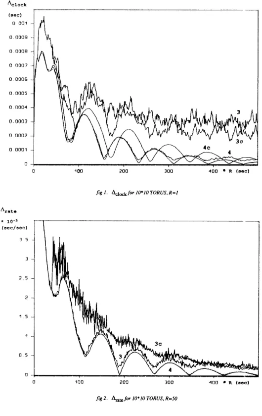
The results of the 10 by 10 torus and 20 nodes ring simulation are presented in figures 1 to 6 below. They show the influence of the non-deterministic message delay on the convergence of the algorithm.

Parameters for the simulations are: R (1, 10,25, 50 sec);

h

(4.103, 4.104 sec-1 : mean dbth = 1 resp. 0.1 msec) and the (yes or no) use of confidence weight factors. In the figures below codes 3,3c, 4 and 4c refer to a simulation result with b4.103, without resp. with confidence and M.104, without resp. with confidence. Each simulation consists of 500 resynchronizations and is carried out twice for e x h set of parameters. Differences in both simulations with the same parameter values were in the order of 10%.

Two values were calculated during the simulations: the maximum clock difference Aclock and maximum rate

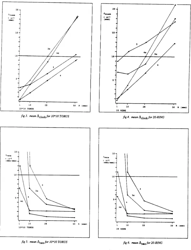
difference Ante. Examples of their behaviour as a function of the number of resynchronizations are presented in figures 1 and 2. The mean value over the last

100 resynchronizations of Adock and Ante are presented in figures 3 to 6.

Discussion.

As expected quick synchronization is obtained for short resynchronization internals: figure 1 shows that for R=l

all curves remain below A = O.ld = 1 msec after about 25

resynchronizations.

Figures 3 and 4 show that Aclock is proportional to R. The influence of the message delay on the mean of Aclock over the last 100 resynchronizations is less than the influence of confidence. The algorithm behaves better without the

use of confidence: With confidence R=25 seems to be the limit to keep clock differences below O.ld msec, whereas

R=50 is possible without confidence. Since there is only a small number of remote clocks, too many of them could easily get a zero confidence weight factor, resulting in poor adjustment of the local clock. Above that the filter indirectly associates a kind of confidence with the calculated global time too (a small a means that a difference is only partially corrected). An optimal relation between the confidence function and the values for a and

p

has not yet been found.

Figure 4 shows that the algorithm behaves a bit worse on the ring than on the torus, probably because there are less neighbours to comect the local time.

Figures 5 and 6 show that Ante does not differ much for torus and ring. For R>10 the mean of Ante over the last 100 resynchronizations is between 10-5 and 10" for both

h's, with or without confidence. For small R the drift Seems to be corrected too frequently. Possibly other values for a and

p

are needed in those cases.

Figures 1 and 2 show that for small delays

Acid

and

hte

have an oscillating behaviour. It is expected that it is

caused by the second order filter, but a suitable explanation has not yet been found.

Conclusion

Simulations on the ring and the torus (both with diameter d=10) show that the proposed algorithm realizes the two requirements stated in the beginning: (1) to bring and

keep Adock below A = O.ld = 1 msec and (2) to decrease Afate.

References

[ ~ r i s t i a n 891

Distributed Computing, 1989, Vol. 3, No. 3, pp. 146-158. [De Carlini 881

Algorithm for Clock Synchronization in Transputer Network ', Software Practice and Experience, 1988, Vol. 18. No.4. April, pp. 331-347. [Kopetz 871

Synchronization in Distributed Real-Time Systems". IEEE Tnursactions (Lamport 781 L a m p & L. "Time. Clocks and the Ordering of Events in a Distributed S stem", Communications of the ACM. 1978. Vol21, No. 7, July, pp. &8-565.

"Synchronizing Clocks in

1985, Vol. 32, No. 4. January. pp. 52-78.

[Machugall 871 MacDougall M.H Simulating Com uter Systems: Techniques and Tools. n;e Ml? Press, 1987, &Press Series in Computer Systems.

[Meijerink 891 Meijerink, G.J., Clock Synchronization in a

distributed Real-time Systems, MSc Thesis, University of Twente, The Netherlands. 1989.

micken 881

synchronization - a programming experiment". Operating Systems Review, 1988. Vol. 22. No. 1, January, pp. 73-78.

[Srikanth 871 Srikanth. T.K. and S. Toueg. '* timal Clock

Synchronization", Journal of the ACM, 1987, Vol. 3 8 0 . 3 . July, pp. 625-645.

[Thambidurai 891 Thambidurai, P.. A.M. Finn, R.M. Kieckhafer and C.J. Walter, "Clock Synchronization in M A P . The nineteenth international symposium on fault tolerant computing, 1989, pp. 142- 149.

Christian, F., "Probalistic clock synchronization", De Carlini, U. and U. Villano, "A Simyle

Kopetz, H. and W. Ochsenreiter, "Clock

on c ~ m p ~ t e r ~ , 1987, Vol. C-36, NO. 8. AUPS~, p ~ . 933-940.

Lam rt, L. and P.M. MelliarSmith. e Presence of Faults". Journal of the ACM, [Lamport 851

'clock ( s e c ) 0 001 0 0009 0 OOOB 0 no07 0 0006 0 0005 0 0004 0,0003 0 0002 0 0001 0 k t e * 10-5 (sec/sec) 3 5 3 2 5 2 1 5 I o s 0 400 R ( s e c ) 0 00 200 300

fig 1 . AClock for 10+10 TORUS, R=l

I

0 100 200 300 400 R ( s e c )

za 1

fig 3 . mean Aclock for 10+10 TORUS

fig 5 . mean Arate for 10+10 TORUS

I

8 I

1 10 2s 50 R (.mal

fig 4. mean Aclock for 20-RING