Aggregating Modalities using MapReduce
Domenico Bianculli1, Carlo Ghezzi2, and Sr ¯dan Krsti´c21 SnT Centre - University of Luxembourg, Luxembourg
2 DEEP-SE group - DEIB - Politecnico di Milano, Italy
{carlo.ghezzi,srdan.krstic}@polimi.it
Abstract. Modern complex software systems produce a large amount of execu-tion data, often stored in logs. These logs can be analyzed using trace checking techniques to check whether the system complies with its requirements specifi-cations. Often these specifications express quantitative properties of the system, which include timing constraints as well as higher-level constraints on the occur-rences of significant events, expressed using aggregate operators.
In this paper we present an algorithm that exploits the MapReduce programming model to check specifications expressed in a metric temporal logic with aggregat-ing modalities, over large execution traces. The algorithm exploits the structure of the formula to parallelize the evaluation, with a significant gain in time. We report on the assesment of the implementation—based on the Hadoop framework—of the proposed algorithm and comment on its scalability.
1
Introduction
Modern software systems, such as service-based applications (SBAs), are built accord-ing to a modular and decentralized architecture, and executed in a distributed environ-ment. Their development and their operation depend on many stakeholders, including the providers of various third-party services and the integrators that realize composite applications by orchestrating third-party services. Service integrators are responsible to the end-users for guaranteeing an adequate level of quality of service, both in terms of functional and non-functional requirements. This new type of software has triggered several research efforts that focus on the specification and verification of SBAs.
In previous work [8], some of the authors presented the results of a field study on property specification patterns [12] used in the context of SBAs, both in industrial and in research settings. The study identified a set of property specification patterns specific to service provisioning. Most of these patterns are characterized by the presence of ag-gregate operations on sequences of events occurring in a given time window, such as “the average distance between pairs of events (e.g., average response time)”, “the num-ber of events in a given time window”, “the average (or maximum) numnum-ber of events in a certain time interval over a certain time window”. This study led to the definition of SOLOIST [9] (SpecificatiOn Language fOr servIce compoSitions inTeractions), a metric temporal logic with new temporal modalities that support aggregate operations
on events occurring in a given time window. The new temporal modalities capture, in a concise way, the new property specification patterns presented in [8].
SOLOIST has been used in the context ofoffline trace checkingof service execution traces. Trace checking (also calledtrace validation[15] orhistory checking[13]) is a procedure for evaluating a formal specification over a log of recorded events produced by a system, i.e., over a temporal evolution of the system. Traces can be produced at run time by a proper monitoring/logging infrastructure, and made available at the end of the service execution to perform offline trace checking. We have proposed procedures [5, 7] for offline checking of service execution traces against requirements specifications written in SOLOIST using bounded satisfiability checking techniques [16]. Each of the procedures has been tailored to specific types of traces, depending on the degree of sparseness of the trace (i.e., the ratio between the number of time instants where significant events occur and those in which they do not). The procedure described in [5] is optimized for sparse traces, while the one presented in [7] is more efficient for dense traces.
Despite these optimizations, our experimental evaluation revealed, in both proce-dures, an intrinsic limitation in their scalability. This limitation is determined by the size of the trace, which can quickly lead to memory saturation. This is a very com-mon problem, because execution traces can easily get very large, depending on the running time captured by the log, the systems the log refers to (e.g., several virtual machines running on a cloud-based infrastructure), and the types of events recorded. For example, granularity can range from high-level events (e.g., sending or receiving messages) to low-level events (e.g., invoking a method on an object). Most log analyz-ers that process data streams [10] or perform data mining [17] only partially solve the problem of checking an event trace against requirements specifications, because of the limited expressiveness of the specification language they support. Indeed, the analysis of a trace may require checking for complex properties, which can refer to specific se-quence of events, conditioned by the occurrence of other event sese-quence(s), possibly with additional constraints on the distance among events, on the number of occurrences of events, and on various aggregate values (e.g., average response time). SOLOIST ad-dresses these limitations as we discussed above.
The recent advent of cloud computing has made it possible to process large amount of data on networked commodity hardware, using a distributed model of computation. One of the most prominent programming models for distributed, parallel computing is MapReduce [11]. The MapReduce model allows developers to process large amount of data by breaking up the analysis into independent tasks, and performing them in parallel on the various nodes of a distributed network infrastructure, while exploiting, at the same time, the locality of the data to reduce unnecessary transmission over the network. However, porting a traditionally-sequential algorithm (like trace checking) into a parallel version that takes advantage of a distributed computation model like MapReduce is a non-trivial task.
The main contribution of this paper is an algorithm that exploits the MapReduce programming model to check large execution traces against requirements specifications written in SOLOIST. The algorithm exploits the structure of a SOLOIST formula to parallelize its evaluation, with significant gain in time. We have implemented the
algo-rithm in Java using the Apache Hadoop framework [2]. We have evaluated the approach in terms of its scalability and with respect to the state of art for trace checking of LTL properties using MapReduce [3].
The rest of the paper is structured as follows. First we provide some background information, introducing SOLOIST in Sect. 2 and then the MapReduce programming model in Sect. 3. Section 4 presents the main contribution of the paper, describing the algorithm for trace checking of SOLOIST properties using the MapReduce program-ming model. Section 5 discusses related work. Section 6 presents the evaluation of the approach, both in terms of scalability and in terms of a comparison with the state of the art for MapReduce-based trace checking of temporal properties. Section 7 provides some concluding remarks.
2
SOLOIST
In this section we provide a brief overview of SOLOIST; for the rationale behind the language and a detailed explanation of its semantics see [9].
The syntax of SOLOIST is defined by the following grammar:φ::=p| ¬φ|φ∧φ| φUIφ|φSIφ|CK./n(φ)|U
K,h
./n(φ)|MK./,nh(φ)|DK./n(φ,φ), where p∈Π, withΠ being a
finite set of atoms. In practice, we use atoms to represent different events of the trace. Iis a nonempty interval overN;./∈ {<,≤,≥, >,=};n,K,hrange overN. Moreover,
for the D modality, we require that the subformulae pair(φ,ψ) evaluate to true in alternation.
TheUIandSImodalities are, respectively, the metric “Until” and “Since” operators.
Additional temporal modalities can be derived using the usual conventions; for exam-ple “Next” is defined asXIφ≡ ⊥UIφ; “Eventually in the Future” asFIφ≡ >UIφand
“Always” asGIφ≡ ¬(FI¬φ), where>means “true” and⊥means “false”. Their past
counterparts can be defined using “Since” modality in a similar way. The remaining modalities are calledaggregatemodalities and are used to express the property speci-fication patterns characterized in [8]. TheCK
./n(φ)modality states a bound (represented
by./n) on the number of occurrences of an eventφin the previousKtime instants; it is also called the “counting” modality. TheUK./,nh(φ)(respectively,MK./,nh(φ)) modality expresses a bound on the average (respectively, maximum) number of occurrences of an eventφ, aggregated over the set of right-aligned adjacent non-overlapping subintervals within a time windowK; it can express properties like “the average/maximum number of events per hour in the last ten hours”. A subtle difference in the semantics of theU andMmodalities is thatMconsiders events in the (possibly empty) tail interval, i.e., the leftmost observation subinterval whose length is less thanh, while theUmodality ignores them. TheDK
./n(φ,ψ)modality expresses a bound on the average time elapsed
between occurrences of pairs of specific adjacent eventsφandψin the previousKtime instants; it can be used to express properties like the average response time of a service.
The formal semantics of SOLOIST is defined on timedω-words [1] over 2Π×
N.
A timed sequence τ =τ0τ1. . . is an infinite sequence of values τi ∈N withτi>0
satisfying τi<τi+1, for alli≥0, i.e., the sequence increases strictly monotonically. A timed ω-word over alphabet 2Π is a pair(
σ,τ)whereσ =σ0σ1. . .is an infinite word over 2Π and
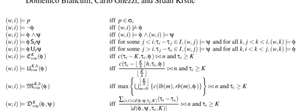
(w,i)|=p iffp∈σi
(w,i)|=¬φ iff(w,i)6|=φ
(w,i)|=φ∧ψ iff(w,i)|=φ∧(w,i)|=ψ
(w,i)|=φSIψ iff for somej<i,τi−τj∈I,(w,j)|=ψand for allk,j<k<i,(w,k)|=φ (w,i)|=φUIψ iff for somej>i,τj−τi∈I,(w,j)|=ψand for allk,i<k<j,(w,k)|=φ (w,i)|=CK ./n(φ) iffc(τi−K,τi,φ)./nandτi≥K (w,i)|=U./K,nh(φ) iff c(τi− b K hch,τi,φ) bK hc ./nandτi≥K (w,i)|=M./K,nh(φ) iff max ( S j K h k m=0{c(lb(m),rb(m),φ)} ) ./nandτi≥K (w,i)|=DK ./n(φ,ψ) iff ∑(s,t)∈d(φ,ψ,τi,K)(τt−τs) |d(φ,ψ,τi,K)| ./nandτi≥K
wherec(τa,τb,φ) =| {s|τa<τs≤τband(w,s)|=φ} |,lb(m) =max{τi−K,τi−(m+1)h},rb(m) =τi−mh, and
d(φ,ψ,τi,K) ={(s,t)|τi−K<τs≤τiand(w,s)|=φ,t=min{u|τs<τu≤τi,(w,u)|=ψ}}
Fig. 1:Formal semantics of SOLOIST
words over the same alphabet. Notice that there is a distinction between the integer positioniin the timedω-word and the corresponding timestampτi. Figure 1 defines
the satisfiability relation(w,i)|=φfor every timedω-wordw, every positioni≥0 and for every SOLOIST formulaφ. For the sake of simplicity, hereafter we express theU modality in terms of theCone, based on this definition:UK./,nh(φ)≡Cb
K hc·h
./n·bK hc
(φ), which can be derived from the semantics in Fig. 1.
We remark that the version of SOLOIST presented here is a restriction of the origi-nal one introduced in [9]: to simplify the presentation in the next sections, we dropped first-order quantification on finite domains and limited the argument of theD modal-ity to only one pair of events; as detailed in [9], these assumptions do not affect the expressiveness of the language.
SOLOIST can be used to express some of the most common specifications found in service-level agreements (SLAs) of SBAs. For example the property: “The aver-age response time of operation A is always less than 5 seconds within any 900 sec-ond time window, before operation B is invoked” can be expressed as: G(Bstart → D900
<5(Astart,Aend)), whereAandBcorrespond to generic service invocations and each
operation has astartand anendevent, denoted with the corresponding subscripts. We now introduce some basic concepts that will be used in the presentation of our distributed trace checking algorithm in Sect. 4. Letφ andψ be SOLOIST formulae. We denote withsub(φ)the set of all subformulae ofφ; notice that foratomicformulae a∈Π, sub(a) =/0. The set ofatomicsubformulae (oratoms) of formulaφ is defined assuba(φ) ={a|a∈sub(φ), sub(a) =/0}. The setsubd(φ) ={α|α∈sub(φ),∀β ∈ sub(φ),α ∈/sub(β)}represents the set of alldirect subformulaeofφ;φ is called the superformulaof all formulae insubd(φ). The notationsupψ(φ)denotes the set of all subformulae ofψ that have formulaφasdirect subformula, i.e.,supψ(φ) ={α |α∈ sub(ψ),φ∈subd(α)}. The subformulae insub(ψ)of a formulaψ form a lattice with
respect to the partial ordering induced by the inclusion in setssupψ(·)andsubd(·), with ψand /0 being thetopandbottomelements of the lattice, respectively. We also introduce
the notion of theheightof a SOLOIST formula, which is defined recursively as: h(φ) =
max{h(ψ)|ψ∈subd(φ)}+1 ifsubd(φ)6=/0
0 otherwise.
We exemplify these concepts using formulaγ≡C40./3(a∧b)U(30,100)¬c.
Hencesub(γ) ={a,b,c,a∧b,¬c,C40
./3(a∧b)}is the set of all subformulae ofγ;suba(γ) = {a,b,c}is the set ofatomsinγ;subd(γ) ={C40./3(a∧b),¬c}is the set of direct subfor-mulae ofγ;supγ(a) =supγ(b) ={a∧b}shows that the sets of superformulae ofaandb inγcoincide; and the height ofγis 3, sinceh(a) =h(b) =h(c) =0,h(¬c) =h(a∧b) = 1,h(C40./3(a∧b)) =2 and thereforeh(γ) =max{h(C40./3(a∧b)),h(¬c)}+1=3.
3
The MapReduce programming model
MapReduce [11] is a programming model for processing and analyzing large data sets using a parallel, distributed infrastructure (generically called “cluster”). At the basis of the MapReduce abstraction there are two functions, map and reduce, that are inspired by (but conceptually different from) the homonymous functions that are typically found in functional programming languages. Themapandreducefunctions are defined by the user; their signatures aremap(k1,v1) → list(k2,v2)and re-duce(k2,list(v2)) → list(v2). The idea of MapReduce is to apply amap func-tion to each logical entity in the input (represented by a key/value pair) in order to com-pute a set of intermediate key/value pairs, and then applying areducefunction to all the values that have the same key in order to combine the derived data appropriately.
Let us illustrate this model with an example that counts the number of occurrences of each word in a large collection of documents; the pseudocode is:
map(String key, String value) //key: document name //value: document contents for each word w in value:
EmitIntermediate(w,"1")
reduce(String key, Iterator values): //key: a word
//values: a list of counts int result = 0
for each v in values: result += ParseInt(v) Emit(AsString(result)
Themapfunction emits list of pairs, each composed of a word and its associated count of occurrences (which is just 1). All emitted pairs are partitioned into groups and sorted according to their key for the reduction phase; in the example, pairs are grouped and sorted according to the word they contain. Thereducefunction sums all the counts (using an iterator to go through the list of counts) emitted for each particular word (i.e., each unique key).
Besides the actual programming model, MapReduce brings in a framework that provides, in a transparent way to developers, parallelization, fault tolerance, locality optimization, and load balancing. The MapReduce framework is responsible for parti-tioning the input data, scheduling and executing theMapandReducetasks (also called mappersandreducers, respectively) on the machines available in the cluster, and for managing the communication and the data transfer among them (usually leveraging a distributed file system).
More in detail, the execution of a MapReduce operation (calledjob) proceeds as follows. First, the framework divides the input into splits of a certain size using an InputReader, generating key/value(k,v)pairs. It then assigns each input split to Map tasks, which are processed in parallel by the nodes in the cluster. A Map task reads the corresponding input split and passes the set of key/value pairs to themapfunction, which generates a set ofintermediatekey/value pairs(k0,v0). Notice that each run of themapfunction is stateless, i.e., the transformation of a single key/value pair does not depend on any other key/value pair. The next phase is calledshuffle and sort: it takes the intermediate data generated by each Map task, sorts them based on the intermediate data generated from other nodes, divides these data into regions to be processed by Reduce tasks, and distributes these data on the nodes where the Reduce tasks will be executed. The division of intermediate data into regions is done by apartitioning function, which depends on the (user-specified) number of Reduce tasks and the key of the intermediate data. Each Reduce task executes thereducefunction, which takes an intermediate key k0and a set of values associated with that key to produce the output data. This output is appended to a final output file for this reduce partition. The output of the MapReduce job will then be available in several files, one for each Reduce task used.
4
Trace checking with MapReduce
Our algorithm for trace checking of SOLOIST properties takes as input a non-empty execution traceT and the SOLOIST formulaΦto be checked. The traceTis finite and can be seen as a time-stamped sequence ofHelements, i.e.,T = (p1,p2, . . . ,pH). Each
of these elements is a triple pi= (i,τi,(a1, . . . ,aPi)), whereiis the position within the
trace,τithe integer timestamp, and(a1, . . . ,aPi)is a list of atoms such thataji∈Π, for
all ji∈ {1, ...Pi},Pi≥1 and for alli∈ {1,2, . . . ,H}.
The algorithm processes the trace iteratively, through subsequent MapReduce passes. The number of MapReduce iterations is equal to height of the SOLOIST formulaΦto be checked. Thel-th iteration (with 1<l≤h(Φ)) of the algorithm receives a set of tuples from the(l−1)-th iteration; these input tuples represent all the positions where the subformulae ofΦhaving heightl−1 hold. Thel-th iteration then determines all the positions where the subformulae ofΦwith heightlhold.
Each iteration consists of three phases: 1) reading and splitting the input; 2) (map) associating each formula with its superformula; 3) (reduce) determining the positions where the superformulae obtained in the previous step hold, given the positions where their subformulae hold. We detail each phase in the rest of this section.
4.1 Input reader
We assume that before the first iteration of the algorithm the input trace is available in the distributed file system of the cluster; this is a realistic assumption since in a distribute setting is possible to collect logs, as long as there is a total order among the timestamps. The input reader at the first iteration reads the trace directly, while in all subsequent iterations input readers read the output of the reducers of the previous iteration.
functionINPUT READERΦ,k,l(Tk) for all(i,τi,A)∈Tkdo T S(i)←τi for alla∈Ado ifa∈suba(Φ)then output(a,i) end if end for end for end function
(a)Input reader algorithm
pi
(a1,i)
. . .
(aPi,i)
Input reader
(b)Data flow of the Input reader
Fig. 2:Input reader
The input reader component of the MapReduce framework is able to process the input trace exploiting some parallelism. Indeed, the MapReduce framework exploits the location information of the different fragments of the trace to parallelize the execution of the input reader. For example, a trace split into n fragments can be processed in parallel using min(n,k)machines, given a cluster withkmachines.
Figure 2b shows how the input reader transforms the trace at the first iteration: for every atomic propositionφthat holds at positioniin the original trace, it outputs a tuple of the form(φ,i). The transformation does not happen in the subsequent iterations, since (as will be shown in Sect. 4.3) the output of the reduce phase has the same form(φ,i). The algorithm in Fig. 2a shows how input reader handles thek-th fragmentTkof the
input traceT. For each time pointiand for each atompthat holds in positioniit creates a tuple(p,i). Moreover, for each time pointi, it updates a globally-shared associative list of timestampsT S. This list is used to associate a timestamp with each time point; its contents are saved in the distributed file system, for use during the reduce phase.
4.2 Mapper
Each tuple generated by an input reader is passed to a mapper at the local node. Map-pers “lift” the formula in the tuple by associating it with all its superformulae in the input formulaΦ. For example, given the formulaΦ ≡(a∧b)∨ ¬a, the tuple(a,5)is associated with formulaea∧band¬a. The reduce phase will then exploit the informa-tion about the direct subformulae to determine all the posiinforma-tions in which a superformula holds.
As shown in Fig. 3, the output of a mapper are tuples of the form((ψ,i),(φ,i))
whereφ is a direct subformulae of ψ andi is the position whereφ holds. For each received tuple of the form(φ,i), the algorithm shown in Fig. 3a loops through all the superformulaeψofφand emits (using the functionoutput) a tuple((ψ,i),(φ,i)).
Notice that the key of the intermediate tuples emitted by the mapper has two parts: this type of key is called acomposite keyand it is used to performsecondary sortingof the intermediate tuples. Secondary sorting performs the sorting using multiple criteria, allowing developers to sort not only by the key, but also “by value”. In our case, we perform secondary sorting based on the position where the subformula holds, in order
functionMAPPERΦ,l((φ,i)) ifl≤h(φ)then
for allψ∈supΦ(φ)do output((ψ,i),(φ,i)) end for
end if end function
(a)Mapper algorithm
(φ,i)
((ψ1,i),(φ,i))
. . .
((ψg,i),(φ,i)) Mapper
(b)Data flow of a Mapper
Fig. 3:Mapper
to decrease the memory used by the reducer. To enable secondary sorting, we need to override the procedure that compares keys, to take into account also the second element of the composite keys when their first elements are equal. We have also modified the key grouping procedure to consider only the first part of the composite key, so that each re-ducer gets all the tuples related to exactly one superformula (as encoded in the first part of the key), sorted in ascending order with respect to the position where subformulae hold (as encoded in the second part of the key).
4.3 Reducer
In the reduce phase, at each iterationl, reducers calculate all positions where subfor-mulae with heightlhold. The total number of reducers running in parallel at thel-th iteration is the minimum between the number of subformulae with heightl in the in-put formulaΦ and the number of machines in the cluster multiplied by the number of reducers available on each node. Each reducer calls an appropriate reduce function depending on the type of formula used as key in the input tuple. The initial data shared by all reducers is the input formulaΦ, the index of the current MapReduce iterationl and the associative map of timestampsTS.
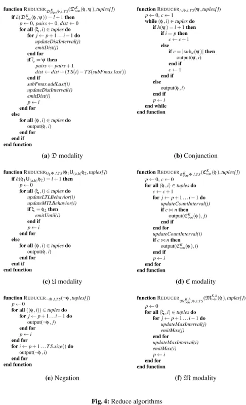
In the rest of this section we present the algorithms of the reduce function defined for SOLOIST connectives and modalities. For space reasons we limit the description to the algorithms for negation (¬) and conjunction (∧), and for the modalitiesUI,CK./n, MK./,nh, andDK./n. The other temporal modalities can be expressed in a way similar to the
UntilmodalityUI. In the various algorithms we use several auxiliary functions whose
pseudocode is available in the extended version of this article [6].
Negation.When the key refers to a negated superformula, the reducer emits a tuple at every position where the subformula does not hold, i.e., at every position that does not occur in the input tuples received from the mappers. The algorithm in Fig. 3e shows how output tuples are emitted. If no tuples are received then the reducer emits tuples at each position. Otherwise, it keeps track of the positioniof the current tuple and the positionpof the previous tuple and emits tuples at positions[p+1,i−1].
Conjunction.We extend the binary∧operator defined in Sect. 2 to any positive arity; this extension does not change the language but improves the conciseness of the formulae. With this extension, conjunction a∧b∧c is represented as a single con-junction with 3 subformulae and has height equal to 1. Tuples(φ,i)received from the mapper may refer to any subformulaφ of a conjunction.
functionREDUCERDK ./n,Φ,l,T S(D K ./n(φ,ψ),tuples[]) ifh(DK ./n(φ,ψ)) =l+1then p←0,pairs←0,dist←0 for all(ξ,i)∈tuplesdo
forj←p+1. . .i−1do updateDistInterval(j) emitDist(j) end for ifξ=ψthen pairs←pairs+1
dist←dist+ (T S(i)−T S(subFmas.last)) end if subFmas.addLast(i) updateDistInterval(i) emitDist(i) p←i end for else
for all(φ,i)∈tuplesdo output(φ,i) end for end if end function
functionREDUCER∧,Φ,l,T S(ψ,tuples[])
p←0,c←1 while(φ,i)∈tuplesdo ifh(ψ) =l+1then ifi=pthen c←c+1 else ifc=|subd(ψ)|then output(ψ,i) end if c←1 end if else output(φ,i) end if p←i end while end function
(a)Dmodality (b)Conjunction
functionREDUCERUI,Φ,l,T S(φ1U(a,b)φ2,tuples[]) ifh(φ1U(a,b)φ2) =l+1then
p←0
for all(ξ,i)∈tuplesdo updateLTLBehavior(i) updateMTLBehavior(i) ifξ=φ2then emitUntil(i) end if p←i end for else
for all(φ,i)∈tuplesdo output(φ,i) end for end if end function functionREDUCERCK ./n,Φ,l,T S(C K ./n(φ),tuples[]) p←0,c←0 for all(φ,i)∈tuplesdo
c←c+1 forj←p+1. . .i−1do updateCountInterval(j) ifc./nthen output(CK ./n(φ),j) end if end for updateCountInterval(i) ifc./nthen output(CK ./n(φ),i) end if p←i end for end function (c)Umodality (d)Cmodality
functionREDUCER¬,Φ,l,T S(¬φ,tuples[])
p←0
for all((φ,i))∈tuplesdo forj←p+1. . .i−1do output(¬φ,j) end for p←i end for fori←p+1. . .T S.size()do output(¬φ,i) end for end function functionREDUCER MK./,nh,Φ,l,T S(M K,h ./n(φ),tuples[]) p←0
for all(ξ,i)∈tuplesdo forj←p+1. . .i−1do updateMaxInterval(j) emitMax(j) end for updateMaxInterval(i) emitMax(i) p←i end for end function
(e)Negation (f)Mmodality
In the algorithm in Fig. 3b we process all the tuples sequentially. First, we check if the height of each subformula is consistent with respect to the iteration in which they are processed. In fact, mappers can emit some tuples before the “right” iteration in which they should be processed, since subformule of a conjunction may have different height. If the heights are not consistent, the reducer re-emits the tuples that appeared early. Since the incoming tuples are sorted by their position, it is enough to use a counter to record how many tuples there are in each positioni. When the value of the counter becomes equal to the arity of the conjunction, its means that all the subformulae hold atiand the reducer can emit the tuple for the conjunction at positioni. Otherwise, we reset the counter and continue.
UImodality.The reduce function for theUntilmodality is shown in Fig. 3c. When
we process tuples with this function, we have to check both the temporal behavior and the metric constraints (in the form of an(a,b)interval) as defined by the semantics of the modality.
Given a formulaφ1U(a,b)φ2, we check whether it can be evaluated in the current iteration, since reducer may receive some tuples early. If this happens, reducer re-emits the tuple, as described above.
The algorithm processes each tuple(φ,i)sequentially. It keeps track of all the po-sitions in the(0,b)time window in the past with respect to the current tuple. For each tuple it calls two auxiliary functions,updateLTLBehaviorand updateMTLBehav-ior. The first function checks whetherφ1holds in all the positions tracked in the(0,b) time window; if this not the case we stop tracing these positions. This guarantee that we only keep track of the position that exhibit the correct temporal semantics of theUntil formula. Afterwards, functionupdateMTLBehaviorchecks the timing constraints and removes positions that are outside of the(0,b)time window. Lastly, ifφ2holds in the position of the current tuple, we call functionemitUntil, which emits anUntiltuple for each position that we track, which is not in the(0,a)time window in the past.
Cmodality.The reduce function for theCmodality is outlined in the algorithm in Fig. 3d. To correctly determine ifCmodality holds, we need to keep track of all the positions in the past time window(0,K). While we sequentially process the tuples, we use variable pto save the position which appeared in the previous tuple. This allows us to consider positions between each consecutive tuple in the inner “for” loop. We call functionupdateCountInterval, which checks if the tracked positions, together with the current one, occur within the time window(0,K); positions that do not fall within the time interval are discarded. Variablecis used to count in how many tracked positions subformulaφ holds. At the end, we compare the value ofcwithnaccording to the./comparison operator; if this comparison is satisfied we emit aCtuple.
Mmodality.The algorithm in Fig. 3f shows when the tuples for theMmodality are emitted. Similarly to theCmodality, we need to keep track of the all positions in the (0,K)time window in the past. Also, the two nested “for” loops make sure that we consider all time positions. For each position we call in sequence function up-dateMaxIntervaland functionemitMax. FunctionupdateMaxIntervalis similar toupdateCountInterval, i.e., it checks whether the tracked positions, together with the current one, occur within the time window (0,K). Function emitMaxcomputes, in the tracked positions, the maximum number of occurrences of the subformula in all
subintervals of lengthh. It compares the computed value to the boundnusing the./ comparison operator; if this comparison is satisfied it emits theMmodality tuple.
Dmodality.The reduce function for theDmodality is shown in Fig. 3a. Similarly to the case of theUImodality, if the heights of the subformulae are not consistent with
the index of the current iteration, the reducer re-emits the corresponding tuples. After that, the incoming tuples are processed in a sequential way and two nested “for” loops guarantee that we consider all time points. We need to keep track of all the positions in the (0,K)time window in the past in which either φ or ψ occurred. Differently from the previous aggregate modalities, we have to consider only the occurrences of φ for which there exists a matching occurrence ψ; for each of these pairs we have to compute the distance. This processing of tuples (and the corresponding atoms and time points that they include) is done by the auxiliary functionupdateDistInterval. Variablespairsanddistkeep track of the number of complete pairs in the current time window and their cumulative distance (computed accessing the globally-shared map TSof timestamps). Finally, by means of the functionemitDist, if there is any pair in the time window, we compare the average distance computed as pairsdist with the boundn using the./comparison operator. If the comparison is satisfied, we emit aDmodality tuple.
5
Related work
To the best of our knowledge, the approach proposed in [3] is the only one that uses MapReduce to perform offline trace checking of temporal properties. The algorithm is conceptually similar to ours as it performs iterations of MapReduce jobs depend-ing on the height of the formula. However, the properties of interest are expressed us-ing LTL. This is only a subset of the properties that can be expressed by SOLOIST. Their implementation of the conjunction and disjunction operators is limited to only two subformulae which increases the height of the formula and results in having more iterations. Intermediate tuples exchanged between mappers and reducers are not sorted by the secondary key, therefore reducers have to keep track of all the positions where the subformulae hold, while our approach tracks only the data that lies in the relevant interval of a metric temporal formula.
Distributed computing infrastructures and/or programming models have also been used for other verification problems. Reference [14] proposes a distributed algorithm for performingmodel checkingof LTLsafety propertieson a network of interconnected workstations. By restricting the verification to safety properties, authors can easily par-allelize a bread-first search algorithm. Reference [4] proposes a parallel version of the well-known fixed-point algorithm for CTL model checking. Given a set of states where a certain formula holds and a transition relation of a Kripke structure, the algorithm computes the set of states where the superformula of a given formula holds though a series of MapReduce iterations, parallelized over the different predecessors of the states in the set. The set is computed when a fixed-point of a predicate transformer is reached as defined by the semantics of each specific CTL modality.
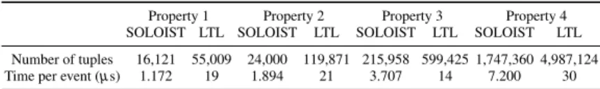
Table 1:Average processing time per tuple for the four properties.
Property 1 Property 2 Property 3 Property 4
SOLOIST LTL SOLOIST LTL SOLOIST LTL SOLOIST LTL
Number of tuples 16,121 55,009 24,000 119,871 215,958 599,425 1,747,360 4,987,124
Time per event (µs) 1.172 19 1.894 21 3.707 14 7.200 30
6
Evaluation
We have implemented the proposed trace checking algorithm in Java using the Hadoop MapReduce framework [2] (version 1.2.1). We executed it on a Windows Azure cloud-based infrastructure where we allocated 10 small virtual machines with 1 CPU core and 1.75 GB of memory. We followed the standard Hadoop guidelines when configuring the cluster: the number of map tasks was set to the number of nodes in the cluster multiplied by 10, and the number of reducers was set to the number of nodes multiplied by 0.9; we used 100 mappers and 9 reducers. We have also enabled JVM reuse for any number of jobs, to minimize the time spent by framework in initializing Java virtual machines. In the rest of this section, we first show how the approach scales with respect to the trace length and how the height of the formula affects the running time and memory. Afterwards, we compare our algorithm to the one presented in [3], designed for LTL.
Scalability. To evaluate scalability of the approach, we considered 4 formulae, with different height:C50000
<10 (a0),D50000<10 (a1,a2),(a0∧(a1∧a2))U(50,200)((a1∧a2)∨a1)and
∃j∈ {0. . .9} ∀i∈ {0. . .8}:G(50,500)(ai,j→X(50,500)(ai+1,j)). Here the∀and∃
quan-tifiers are used as a shorthand notation to predicate on finite domains: for example, ∀i∈ {1,2,3}:aiis equivalent toa1∧a2∧a3. We generated random traces with a num-ber of time instants varying from 10000 to 350000. For each time instant, we randomly generated with a uniform distribution up to 100 distinct events (i.e.,atomic proposi-tions). Hence, we evaluated our algorithm for a maximum number of events up to 35 millions. The time span between the first and the last timestamp was 578.7 days on average, with a granularity of one second.
Figure 5 shows the total time and the memory used by the MapReduce job run to check the four formulae on the generated traces. FormulaeC50000<10 (a0)andD50000<10 (a1,a2) needed one iteration to be evaluated (shown in Fig. 5a and Fig. 5b). In both cases, the time taken to check the formula increases linearly with respect to the trace length; this happens because reducers need to process more tuples. As for the linear increase in memory usage, for modalitiesCandDreducers have to keep track of all the tuples in the window of lengthKtime units and the more time points there are the moredense the time window becomes, with a consequent increase in memory usage. As for the checking of the other two formulae (shown in Fig. 5c and Fig. 5d), more iterations were needed because of the height of the formulae. Also in this case, the time taken by each iteration tends to increase as the length of the trace increases; the memory usage is con-stant since the formulae considered here do not contain aggregate modalities. Notice the increase of time and memory from Fig. 5c to Fig. 5d: this is due to the expansion of the quantifiers in formula∃j∈ {0. . .9} ∀i∈ {0. . .8}:G(50,500)(ai,j→X(50,500)(ai+1,j)).
0 1 2 3 4
·105
20 30 40
Length of the traceH
T ime (s) Iteration 1 0 1 2 3 4 ·105 800 850 900
Length of the traceH
Memory (MB) Iteration 1 (a)Formula:C50000<10 (a0) 0 1 2 3 4 ·105 20 30 40
Length of the traceH
T ime (s) Iteration 1 0 1 2 3 4 ·105 800 850 900 950
Length of the traceH
Memory (MB) Iteration 1 (b)Formula:D50000<10 (a1,a2) 0 1 2 3 4 5 ·105 40 60 80
Length of the traceH
T ime (s) Iteration 1 Iteration 2 Iteration 3 0 1 2 3 4 5 ·105 1,000 2,000 3,000
Length of the traceH
Memory (MB) Iteration 1 Iteration 2 Iteration 3 (c)Formula:(a0∧(a1∧a2))U(50,200)((a1∧a2)∨a1) 0 1 2 3 ·105 0 500 1,000 1,500
Length of the traceH
T ime (s) Iteration 1 Iteration 2 Iteration 3 Iteration 4 Iteration 5 0 1 2 3 ·105 0 2,000 4,000 6,000
Length of the traceH
Memory (MB) Iteration 1 Iteration 2 Iteration 3 Iteration 4 Iteration 5 (d)Formula:∃j∈ {0. . .9} ∀i∈ {0. . .8}:G(50,500)(ai,j→X(50,500)(ai+1,j))
Comparison with the LTL approach [3]. We compare our approach to the one pre-sented in [3], which focuses on trace checking of LTL properties using MapReduce; for this comparison we considered the LTL layer included in SOLOIST by means of theUntilmodality. Although the focus of our work was on implementing the semantics of SOLOIST aggregate modalities, we also introduces some improvements in the LTL layer of SOLOIST. First, we exploited composite keys and secondary sorting as pro-vided by the MapReduce framework to reduce the memory used by reducers. We also extended the binary∧and∨operators to support any positive arity.
We compared the two approaches by checking the following formulae:
1) G(50,500)(¬a0); 2) G(50,500)(a0→X(50,500)(a1)); 3) ∀i∈ {0. . .8}:G(50,500)(ai →
X(50,500)(ai+1)); and 4)∃j∈ {0. . .9} ∀i∈ {0. . .8}:G(50,500)(ai,j→X(50,500)(ai+1,j)).
The height of these formulae are 2, 3, 4 and 5, respectively. This admittedly gives our approach a significant advantage since in [3] the restriction for the∧and∨operators to have an arity fixed to 2 results in a larger height for formulae 3 and 4. We randomly generated traces of variable length, ranging from 1000 to 100000 time instants, with up to 100 events per time instant. With this configuration, a trace can contain potentially up to 10 million events. We chose to have up to 100 events per time instant to match the configuration proposed in [3], where there are 10 parameters per formula that can take 10 possible values. We generated 500 traces. The time needed by our algorithm to check each of the four formulae, averaged over the different traces, was 52.83, 85.38, 167.1 and 324.53 seconds, respectively. We do not report the time taken by the ap-proach proposed in [3] since the article does not report any statistics from the run of an actual implementation, but only metrics determined by a simulation. Table 1 shows the average number of tuples generated by the algorithm for each formulae. The number of tuples is calculated as the sum of all input tuples for mappers at each iterations in a single trace checking run. The table also shows the average time needed to process a single event in the trace. This time is computed as the total processing time divided by the number of time instants in the trace, averaged over the different trace checking runs. The SOLOIST column refers to the data obtained by running our algorithm, while the LTL column refers to data reported in [3], obtained with a simulation. Our algo-rithm performs better both in terms of the number of generated tuples and in terms of processing time.
7
Conclusion and Future Work
In this paper we present an algorithm based on the MapReduce programming model that checks large execution traces against specifications written in SOLOIST. The ex-perimental results in terms of scalability and comparison with the state of the art are encouraging and show that the algorithm can be effectively applied in realistic settings. A limitation of the algorithm is that reducers (that implement the semantics of tem-poral and aggregate operators) need to keep track of the positions relevant to the time window specified in the formula. In the future, we will investigate how this information may be split into smaller and more manageable parts that may be processed separately, while preserving the original semantics of the operators.
Acknowledgments. This work has been partially supported by the National Research Fund, Luxembourg (FNR/P10/03).
References
1. Alur, R., Dill, D.L.: A theory of timed automata. Theoreotical Computer Science 126(2), 183–235 (Apr 1994)
2. Apache Software Foundation: Hadoop MapReduce. http://hadoop.apache.org/
mapreduce/
3. Barre, B., Klein, M., Soucy-Boivin, M., Ollivier, P.A., Hallé, S.: MapReduce for parallel trace validation of LTL properties. In: Proc. of RV 2012. LNCS, vol. 7687, pp. 184–198. Springer (2012)
4. Bellettini, C., Camilli, M., Capra, L., Monga, M.: Distributed CTL model checking in the
cloud. Tech. Rep. 1310.6670, Cornell University (Oct 2013),http://arxiv.org/abs/
1310.6670
5. Bersani, M.M., Bianculli, D., Ghezzi, C., Krsti´c, S., San Pietro, P.: SMT-based checking of SOLOIST over sparse traces. In: Proc. of FASE 2014. LNCS, vol. 8411, pp. 276–290. Springer (April 2014)
6. Bianculli, D., Ghezzi, C., Krsti´c, S.: Trace checking of metric temporal logic with
aggregat-ing modalities usaggregat-ing MapReduce (2014),http://hdl.handle.net/10993/16806,
ex-tended version
7. Bianculli, D., Ghezzi, C., Krsti´c, S., San Pietro, P.: From SOLOIST to CLTLB(D):
Check-ing quantitative properties of service-based applications. Tech. Rep. 2013.26, Politecnico di Milano - Dipartimento di Elettronica, Informazione e Bioingegneria (October 2013) 8. Bianculli, D., Ghezzi, C., Pautasso, C., Senti, P.: Specification patterns from research to
industry: a case study in service-based applications. In: Proc. of ICSE 2012. pp. 968–976. IEEE Computer Society (2012)
9. Bianculli, D., Ghezzi, C., San Pietro, P.: The tale of SOLOIST: a specification language for service compositions interactions. In: Proc. of FACS’12. LNCS, vol. 7684, pp. 55–72. Springer (2013)
10. Cugola, G., Margara, A.: Complex event processing with T-REX. J. Syst. Softw. 85(8), 1709– 1728 (Aug 2012)
11. Dean, J., Ghemawat, S.: MapReduce: Simplified data processing on large clusters. Commun. ACM 51(1), 107–113 (Jan 2008)
12. Dwyer, M.B., Avrunin, G.S., Corbett, J.C.: Property specification patterns for finite-state verification. In: Proc. of FMSP ’98. pp. 7–15. ACM (1998)
13. Felder, M., Morzenti, A.: Validating real-time systems by history-checking TRIO specifica-tions. ACM Trans. Softw. Eng. Methodol. 3(4), 308–339 (Oct 1994)
14. Lerda, F., Sisto, R.: Distributed-memory model checking with SPIN. In: Proc. of SPIN 1999. LNCS, vol. 1680, pp. 22–39. Springer (1999)
15. Mrad, A., Ahmed, S., Hallé, S., Beaudet, E.: Babeltrace: A collection of transducers for trace validation. In: Proc. of RV 2012. LNCS, vol. 7687, pp. 126–130. Springer (2013)
16. Pradella, M., Morzenti, A., San Pietro, P.: Bounded satisfiability checking of metric temporal logic specifications. ACM Trans. Softw. Eng. Methodol. 22(3), 20:1–20:54 (Jul 2013) 17. Verbeek, H., Buijs, J., Dongen, B., Aalst, W.: XES, XESame, and ProM 6. In: Proc. CAISE