Reducing Student Loan Debt Through Parents’ College Savings

(1)

Campus Box 1196 One Brookings Drive St. Louis, MO 63130-9906  (314) 935.7433  csd.wustl.edu

Reducing Student Loan Debt

through Parents’ College Savings

William Elliott, PhD

University of Kansas, School of Social Welfare

Ilsung Nam, PhD

University of Kansas, School of Social Welfare

2013

CSD Working Paper

No. 13-07

(2)

Acknowledgments

Support for this report comes from the Citi Foundation. Other funders of research on college savings include the Ford Foundation, the Charles Stewart Mott Foundation, and Lumina Foundation for Education. The authors thank Margaret Clancy, Michael Sherraden, and Tiffany Trautwein at the Center for Social Development at Washington University in St. Louis for suggestions, reviews, and editing assistance.

(3)

Reducing Student Loan Debt through Parents’

College Savings

One policy rationale for promoting Child Development Accounts (CDAs) is that they may help reduce college debt, but no research provides evidence of this. Research does suggest that high-dollar student loans ($10,000 or more) can reduce the probability that lower income students in particular persist in and graduate from college. In this study, we find evidence to suggest that parents’ college savings may reduce the probability that students accrue high-dollar student loan debt across all income levels with the exception of high-income students. Based on this and evidence from separate research on small-dollar children’s savings accounts, we suggest that it is important for policies and programs to clearly state their goals. For example, if the goal is to improve expectations for attending and graduating from college or to increase educational attainment, small-dollar children’s savings accounts might make a difference. However, if the goal is to reduce college debt, programs must help children accumulate enough savings to reduce reliance on college loans.

Keywords: Child Development Accounts (CDAs), saving, college enrollment, student loans, college debt

Introduction

The College Board (2012a), which produces an annual report tracking college costs, estimates the total cost of college attendance and room and board at an in-state, public four-year college for the 2012–13 school year is $8,655, an increase of 4.8% from the prior school year. Total cost of a private four-year college also rose by 4.2% in 2012–13 to $29,056 (College Board, 2012a).

Researchers find that increasing college costs have a negative impact on college enrollment decisions (Heller, 1997; Leslie & Brinkman, 1988; McPherson & Schapiro, 1998). McPherson and Schapiro (1998) estimate that a $150 net cost increase (in 1993–1994 dollars) results in a 1.6 percentage-point reduction in enrollment among low-income students. Further compounding the problem is the decline in wages (in inflation-adjusted dollars) for bottom income groups (College Board, 2012a). According to the College Board (2012a), family income declined in 2011 by 5% for the poorest 20% of families.

Shifting the Burden of Paying for College from Society to Students

In addition to rising college costs and stagnant or decreasing family wages, changing federal and state policies are pressuring students to rely more on borrowing. Since the late 1970s, the federal government increasingly has attempted to promote equal access through adoption of policies that make college loans accessible to more students (Heller, 2008). Most recently, the Health Care and Education Reconciliation Act (2010) routed all federal loans through the Direct Loan program, making it easier for students and families to borrow directly from the U.S. Department of Education.

Another important change in financial aid policy is the shift from need-based aid to merit-based aid (Woo & Choy, 2011). Need-based aid is determined solely by assets and income (i.e., financial need) of prospective students and their families. Factors such as test scores have no bearing on the aid decision. Merit-based aid—most commonly scholarships—often is awarded based on test scores. Students with little financial need have the same entitlement to merit-based aid as students with high

(4)

levels of financial need. Woo and Choy (2011) find that the proportion of undergraduates receiving merit-based aid rose from 6% in 1995–1996 to 14% in 2007–2008. Further, research suggests that merit-based aid is awarded disproportionately to students from higher income families (Woo & Choy, 2011) and has done little to improve college enrollment rates among low-income and minority students (Marin, 2002).

Another change is the role that society plays—largely through providing scholarship and grants—in financing college. Elliott and Friedline (2012) find that students might carry a larger proportion of the college cost burden than society through student loans, savings, job earnings, or federal work study programs. They also find that the college cost burden might vary by race, income level (which is the focus of this paper), and length of college program. Regarding four-year college enrollment, Elliott and Friedline find that the college cost burden is lowest among the lowest income group but highest among the middle-income group. Moreover, they find evidence to suggest that parents’ college savings may help lower the burden on students.

Growing amounts of student debt

Americans see student loans as investments that support long-term achievement (Cunningham & Santiago, 2008), but this borrowing has real costs for students in the amount of debt with which they leave college. During the 2011–2012 school year, 37% of all undergraduate financial aid received ($70.8 billion) came from federal loans (College Board, 2012b). The next highest sources were federal Pell grants (19%) and institutional grants (18%). The percentage of undergraduate students who obtained federal loans increased from 23% in 2001–2002 to 35% in 2011–2012. In 2010–2011, nearly 57% of public four-year college students graduated with debt (The College Board, 2012b). On average, students who attended public four-year colleges borrowed $23,800. Total borrowing for college hit $113.4 billion for the 2011–2012 school year, up 24% from 2007 (College Board, 2012b).

Too much debt may have undesired affects

As a policy mechanism, student loans are designed to ensure that more students have access to college by providing additional funds at the time of enrollment. However, research suggests that after a certain level, student loans might not produce the desired effect of increased enrollment and graduation rates (Dwyer, McCloud, & Hodson, 2012; Heller, 2008). If this is true, simply continuing to increase the amount of loans available to students might not produce the desired effects, and other complementary financial aid policies might be necessary.

Heller (2008) concludes after a literature review that very little evidence suggests loans improve outcomes. Similarly, Cofer and Somers (2001) suggest that larger amounts are counterproductive and fail to meet the goal of making college accessible to more students while smaller loan amounts might have positive effects. Dwyer, McCloud, and Hodson (2012) find that debt below $10,000 has a positive relationship with college completion, while debt above $10,000 has a negative relationship with college completion for the bottom 75% of the income distribution in their study. Other

researchers find evidence that loan debt may have a more negative impact on college persistence during the first year than in subsequent years (Dowd & Coury, 2006; Kim, 2007).

Further, prior research suggests that student loans may be a more effective strategy for middle- and high-income students because of low-income students’ aversion to borrowing (Campaigne &

(5)

Hossler, 1998; Paulsen & St. John, 2002). Similar findings exist with regard to race. Perna (2000) finds that student loans have a negative effect on enrollment in four-year college for Black students, and she attributes this in part to an aversion to borrowing.

Interestingly, evidence suggests that loans plus grants might be a more effective strategy than loans by themselves. For example, Hu and St. John (2001) examine different types of financial aid and find that when combined with grants, loans have a more positive effect on persistence than loans only among different racial groups. This led Heller (2008) to conclude, ―If grant aid were proportionally higher, then loans might provide more of a positive impact on college participation‖ (p. 49). However, with the shift toward merit-based aid for determining eligibility for grants and

scholarships, some researchers suggest that grants increasingly benefit middle- and upper income students (Woo & Choy, 2011).

The growing belief among policymakers is that the individual—who benefits most from attending college—should bear more personal responsibility. Thus, there might be very little political will to continue to increase the number of scholarships and grants available to students. Given this, there may be need for an innovation in financial aid that not only aligns with the notion of individual responsibility but also augments student loans. Asset accumulation strategies, such as Child

Development Accounts (CDAs), might be just such an innovation within the financial aid system. CDAs might serve as a policy vehicle for allocating intellectual and material resources to low- and moderate-income children. Unlike basic savings accounts, CDAs leverage investments by

individuals, families, and sometimes third parties (e.g., initial deposits, incentives, matches). CDAs align with the ideals of personal responsibility because they require students and their families to help pay for college by saving.

Saving and the Potential for Augmenting the Capacity of Student Loans

In May of 2012, the Department of Education (DOE) announced a college savings account research demonstration project that will test CDAs as part of the Gaining Early Awareness and Readiness for Undergraduate Programs (GEAR UP) initiative. The demonstration will test the effectiveness of pairing new federally supported college savings accounts with GEAR UP activities against the effectiveness of standard GEAR UP activities that do not include college savings accounts. They initially will allocate $8.7 million already appropriated to support the demonstration.1

Researchers who study CDAs suggest that they have both direct effects (e.g., reducing the price of college by providing students with money to pay for college) and indirect effects (e.g., improving engagement in school prior to college by making college appear within reach) (Elliott, Choi, Destin, & Kim, 2011; Elliott & Nam, in press). Researchers also find that saving is associated with college enrollment (Elliott & Beverly, 2011a), college persistence (Elliott & Beverly, 2011b), and college graduation (Elliott, in press). Evidence suggests that savings might be more beneficial than grants because they help students accumulate assets that remain well after leaving college (Elliott, Rifenbark, Webley, Friedline, & Nam, 2012; Friedline & Elliott, in press).

While some evidence suggests that assets—such as net worth and savings accounts—do have positive relationships with college enrollment and graduation (see Elliott, Destin, & Friedline, 2011),

(6)

there is little information about whether CDAs can help reduce student debt. In this study, we focus on the role of parents’ savings for their children’s college education and its potential to reduce the amount of debt students are forced to assume in order to attend college. We focus on savings accounts because they most closely resemble CDAs, which can be thought of as savings accounts for children. Because CDAs allow not only children but also parents and others to save in the

accounts, Loke and Sherraden (2009) suggest that they might have a ―…multiplier effect by engaging the larger family in the asset-accumulation process‖ (p. 119).

Research Question

In this study, we ask whether parents’ savings for their children’s college education are associated with reduced college debt. Research suggests that the decision to borrow for college is a complex process (e.g., Dowd & Coury, 2006; Kinzie et al., 2004). Students are provided with many alternative financial aid packages from different schools, but research databases provide very little information about the financing alternatives from which the student had to choose. As a result, developing highly explanatory models (i.e., models that explain a lot of the difference in why one child chooses to borrow for college and a similarly situated child does not) can be difficult. Moreover, we find no research outside of descriptive studies that predict how much debt students accumulate while in college or whether having parents with college savings is predictive of the amount of debt incurred. Research on financial aid has focused largely on students’ aversion to taking out loans, loans’

predictability of college attainment, and predictors of loan default. Research on CDAs has focused primarily on educational attainment and children’s expectations for attending college, but one of the policy arguments for adopting CDAs is that they can help reduce college debt. Given this, it seems important to undertake a study to test whether an association exists between assets—in this case, parents’ college savings—and college debt while controlling for factors believed to play a role in whether students borrow to pay for college.

Methods Dataset

This study uses longitudinal data from the Educational Longitudinal Survey of 2002 (ELS:2002) made available to the public by the National Center for Education Statistics (NCES). The survey began in 2002 when students were in 10th_{grade, and follow-up waves took place in 2004 and 2006.}

Its purpose was to follow students as they progressed through high school and transitioned to postsecondary education or the labor market and is an ideal dataset to test whether early experiences or resources predicted later outcomes.

The ELS:2002 aimed to present a holistic picture of student achievement by gathering information from multiple sources. Students, their parents, teachers, librarians, and principals provided

information regarding students’ average grades, math achievement, and educational expectations and school resources and curriculum, teacher experience, student and parent work/employment, and students’ post-high school enrollment in college. Dependent variables in this study are from the 2006 wave and independent variables are from the 2002 and 2004 waves.

(7)

Study Sample

The final sample of this study is restricted to students who were in the 2002 10th_{grade cohort, and}

the 2006 ELS samples (i.e., those who answered the follow-up questionnaires), graduated high school, and attended a four-year college. American Indian (0.8%) and biracial students (4.5%) were eliminated from the analysis due to small sample sizes. We also restricted the sample to students who started college between July and December 2004 and students who had finished or were still in college in 2006 at the time of the last ELS interview. After these restrictions were applied, the full sample included 4,963 students. Four subsamples also were drawn from the full sample based on household income level: 860 low-income ($35,000 or below) students, 1,235 moderate-income ($35,001–$75,000) students, 629 middle-income ($75,001–$100,000) students, and 951 high-income ($100,001 or higher) students.

Student Variables

All control variables—with exception of dependent status, student’s income, and expected student loan debt in the future, which were measured in 2006—were measured in the 2002 or 2004 waves of the ELS. The outcome variable—amount of student loan debt—was measured in 2006.

Student’s income

This is a categorical variable indicating total 2005 job earnings: 1 = less than $1,000, 2 = $1,000– $2,999, 3 = $3,000–$5,999, 4 = $6,000–$9,999, 5 = $10,000–$14,999, 6 = $15,000–$19,999, 7 = $20,000 or more. This was collapsed into a five-level variable to more equally distribute the sample across the different categories: 0 = less than $1,000, 1 = $1,000–$2,999, 2 = $3,000–$5,999, 3 = $6,000–$9,999, 4 = $10,000 or more.

Student race/ethnicity

The variable representing race included seven categories in the ELS:2002. American Indian or Alaska Native and more than one race were not included in this analysis due to small sample sizes, and Hispanic and Latino were combined. Four categories were included in the final analysis: White = 0, Black = 1, Latino/Hispanic = 2, and Asian = 3.

Gender

Student’s gender is a dichotomous variable: 1 = male, 0 = female. Student GPA

Students’ grade point average (GPA) is a categorical variable that averages grades for all coursework in 9th_{through 12}th_{grades. There are seven categories: 0 = 0.00–1.00, 1 = 1.01–1.50, 2 = 1.51–2.00, 3}

= 2.01–2.50, 4 = 2.51–3.00, 5 = 3.01–3.50, and 6 = 3.51–4.00. We collapsed categories 0–2 into one due to small frequencies (36, 156, and 782, respectively).

College costs

Students were asked how important low costs (e.g., of tuition, books, room and board) were for choosing a school. Responses were dichotomized: 1 = very important, 0 = not very important.

(8)

Financial aid

Students were asked how important the availability of financial aid was for choosing a school. Responses were dichotomized: 1 = very important, 0 = not very important.

Amount student expects to borrow

Students were asked the amount they expected in undergraduate student loans in the future. The amount expected to borrow is a categorical variable: 1 = $0–1,999, 2 = $2,000–3,999, 3 = $4,000– 5,999, 4 = $6,000–7,999, 5 = $8,000–9,999, 6 = $10,000–14,999, 7 = $15,000–19,999, 8 = $20,000 or more. In this study, expected student loan amount was collapsed into a three-level variable: 0 = $0–$9,999, 1 = $10,000–$19,999, 2 = $20,000 or more.

Parent/household variables

Household income

In the ELS:2002, household income included 13 distinct levels. For this study, the levels of household income were combined into four levels: 0 = low-income ($0–$20,000), 1 = moderate-income ($20,001–$50,000), 2 = middle-moderate-income ($50,001-$100,000), and 3 = high-moderate-income ($100,001 or higher). The levels were chosen, in part, to keep relatively equal cases in each category while maintaining important distinctions between income groups.

Parent education level

Parent education level is equivalent to whichever parent’s is higher and includes eight distinct levels. The eight levels were collapsed into three for the final analysis: 0 = high school diploma or less, 1 = some college, 2 = four-year college degree or higher.

Number of siblings

Number of siblings was a continuous variable that ranged from 0–7. We collapsed families with 4–7 siblings into the same category because of small frequencies with a new range of 0–4.

Secondary school variables

College counseling

This is a dichotomous variable that indicates whether the student had gone to the counselor for college entrance information: 1 = yes, 0 = no.

Percentage of students who attended a four-year college

Percentage of 2003 graduates from high school that went to a four-year college (i.e., this is the percentage from a child’s high school when the child was in 11th_{grade): 1 = none, 2 = 1%–10%, 3 =}

11%–24%, 4 = 25%–49%, 5 = 50%–74%, 6 = 75%–100%. Categories 1–4 were collapsed into one category to help balance the sample and because we felt 50% or more would represent a high level of students attending four-year colleges.

(9)

University variables

Dependent status

This is a dichotomous variable that indicates whether students lived with their parents in 2006: 1 = yes, 0 = no.

College selectivity

The following categories made up the college selectivity variable: 1 = public, four-year or above; 2 = private, not-for-profit, four-year; 3 = private, for-profit, four-year; 4 = public, two-year; 5 = private, not-for-profit, two-year; 6 = private, for-profit, two-year; 7 = public, less than two-year; 8 = private, not-for-profit, less than two-year; 9 = private, for-profit, less than two-year. Due to sample

restrictions, only categories that applied to four-year college attendance (1, 2, and 3) were applicable. Categories 2 and 3 were collapsed to make a dichotomous variable: 0 = public, four-year; 1 = private, four-year).

Applied for financial aid

Students were asked if they applied for financial aid, which resulted in a dichotomous variable: 1 = yes, 0 = no.

Savings or earnings, grants, or parents’ college loans

Students were asked if they paid for postsecondary education with savings or earnings, grants, or parents’ college loans. All three variables were dichotomous: 1 = yes, 0 = no.

Out of state

This is a dichotomous variable that indicates whether the student attended college in the state where they lived: 1 = yes, 0 = no.

Variable of interest

Parents’ college savings accounts

Thevariable of interest came from a survey question that asked parents whether they were

financially preparing to pay for their children to attend college by starting a savings account: 1 = yes, 0 = no.

Outcome Variable

Amount borrowed

The outcome variable of amount borrowed was drawn from the 2006 wave and was a categorical variable: 1 = $0–$1,999, 2 = $2,000–$3,999, 3 = $4,000–$5,999, 4 = $6,000–$7,999, 5 = $8,000– $9,999, 6 = $10,000–$14,999, 7 = $15,000–$19,999, 8 = $20,000 or more.2_{In this study, we created}

a three-level variable: (0 = did not borrow, 1 = $0–$9,999, 2 = $10,000 or more. The ―did not

2_{Dr. Isaiah Lee O’Rear at the National Center for Education Statistics informed us that students who indicated they}

(10)

borrow‖ category included students who skipped the amount borrowed question.3_{These categories}

were chosen based on research that suggests loan debt of $10,000 or more has a negative effect on college attainment (Dwyer et al., 2012).

Analysis Plan

We usedtwo steps—with no problems of multicollinearity—to produce and analyze results for predictors of student college loan debt. The first step was to conduct propensity score analyses for parents with a savings account for their child’s college education (i.e., treated cases) and parents without a savings account for their child’s college education (i.e., non-treated cases). We used two propensity score analyses (i.e., pair matching and propensity score weighting) to cross-validate the results from the two models that adjust selection bias given the observed covariates.

The second step was to create four subgroups (low-income, moderate-income, middle-income, and high-income) using the family income variable and estimating multinomial logistic regressions for each subgroup. Logistic regressions are estimated, and propensity score matching is not used for the subgroups because of sample size. Matching further reduces sample size and power. Data analysis steps were conducted using STATA (version 12).

Propensity score analyses

Propensity score analysis balances the treatment group (i.e., those with savings accounts) on

covariates to get more accurate estimates of the effects of treatment. This method involves matching and weighting cases to create new samples and performing covariate balance checks (D’Agostino, 1998). Following the estimation of the propensity scores, we used two methods of propensity score analysis, including nearest neighbor with caliper match and propensity score weighting. Matching typically reduces the sample size due to the inability to match all treated and non-treated

observations (Guo & Fraser, 2010; Rosenbaum, 2002; Rosenbaum & Rubin, 1985), which could result in a loss of a statistical power of the treatment effect on outcome estimation. Propensity score weighting was used as a non-sample-reducing correction to selection bias.

Propensity score estimation

Logistic regressions were done to estimate propensity scores (i.e., the predicted probability of parents having a savings account for their child’s college education in 2002). Prior to estimating the propensity scores, we conducted a series of logistic regressions to determine the covariates affecting selection bias. The results of these tests (Table 1) reveal significant differences among most

covariates. Table 2 provides unadjusted descriptive statistics.

3_{Dr. Isaiah Lee O’Rear also informed us that legitimate skips could be treated as having responded “did not}

(11)

Table 1. Full Sample Covariate Balance Checks

Before matching (N = 3675) After matching (N = 2661) ATT weighting (N = 3675)

Student variables β SE β SE β SE Income $0–$999 (reference) Income $1,000–$2,999 -.032 .112 .029 .140 -.117 .100 Income $3,000–$5,999 -.043 .117 .020 .138 -.041 .104 Income $6,000–$9,999 -.279 * .132 .131 .159 -.004 .123 Income $10,000 or higher -.473 ** .150 .025 .183 .032 .141 White (reference) Black -.212 .132 .012 .156 -.005 .124 Latino/Hispanic -.597 * .147 .028 .179 -.076 .146 Asian .036 .132 -.044 .159 -.048 .131 Male -.167 .810 -.023 .097 .028 .072

GPA 2.00 or lower (reference)

GPA 2.01–2.50 -.162 .233 -.022 .277 -.409 .212

GPA 2.51–3.00 -.120 .194 -.063 .224 -.238 .174

GPA 3.01–3.50 .038 .188 .072 .217 -.282 .168

GPA 3.51–4.00 .132 .184 -.055 .215 -.213 .164

Low college costs very important -330 *** .090 .086 .107 .059 .081

Financial aid very important -.622 *** .085 .034 .094 .110 .072

Expected to borrow $0–$9,999 (reference)

Expected to borrow $10,000–$19,999 -.549 *** .114 .097 .141 .074 .104

Expected to borrow $20,000 or more -.412 *** .107 -.077 .124 -.012 .098

Parent/Household variables

Low-income ($35,000 or below) (reference)

Moderate-income ($35,001–$75,00) .382 *** .099 -.055 .122 -.097 .082

Middle-income ($75,001–$100,000) .926 *** .124 .026 .143 -.021 .104

High-income ($100,001 or higher) 1.334 *** .117 -.244 .139 -.168 .095

Head of household had high school education or less (reference)

Head of household had some college .603 *** .150 .109 .185 -.057 .130

Head of household had two-year college degree .487 ** .174 .254 .212 .075 .156

Head of household had four-year college degree or higher 1.201 *** .126 .113 .153 -.084 .110

0 or 1 sibling (reference)

2 siblings .292 * .113 .040 .136 -.148 .102

3 siblings .051 .120 .065 .148 -.069 .110

4 or more siblings -.226 .138 -.011 .165 -.046 .122

Secondary school variables

Received college counseling while in high school .026 .077 -.059 .089 -.016 .075

Percentage of students from high school who attended four-year college .284 ** .084 -.008 .094 -.135 .077

College/University variables

Lived with parents (independent status) -.494 *** .095 .065 .119 .005 .088

Attended private four-year college .146 .079 -.076 .095 -.104 .075

Applied for financial aid -.611 *** .107 .119 .117 .184* .090

Paid for college with savings or earnings -.125 .079 -.003 .093 .014 .072

Paid for college with grants -.440 *** .082 .100 .098 .042 .073

Paid for college with parent loans -.118 .085 -.061 .102 -.061 .080

Out-of-state student .401 .085 -.096 .100 -106 .083

Note. β = regression coefficients; SE = standard error. *p < .05; **p < .01; ***p < .001.

(12)

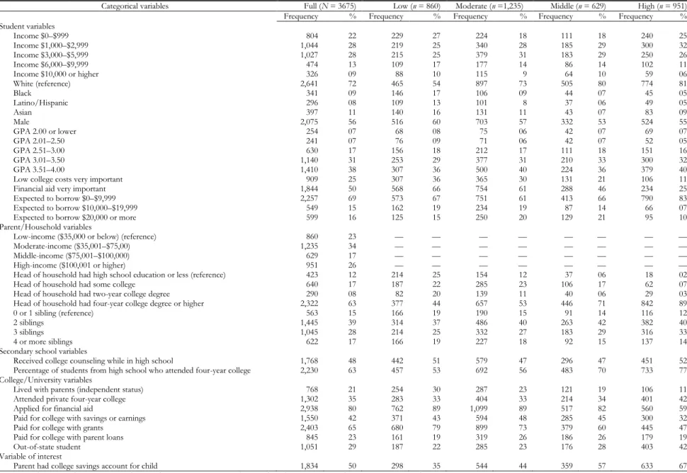
Table 2. Unadjusted descriptive statistics

Categorical variables Full (N = 3675) Low (n = 860) Moderate (n =1,235) Middle (n = 629) High (n = 951)

Frequency % Frequency % Frequency % Frequency % Frequency %

Student variables Income $0–$999 804 22 229 27 224 18 111 18 240 25 Income $1,000–$2,999 1,044 28 219 25 340 28 185 29 300 32 Income $3,000–$5,999 1,027 28 215 25 379 31 183 29 250 26 Income $6,000–$9,999 474 13 109 17 177 14 86 14 102 11 Income $10,000 or higher 326 09 88 10 115 9 64 10 59 06 White (reference) 2,641 72 465 54 897 73 505 80 774 81 Black 341 09 146 17 106 09 44 07 45 05 Latino/Hispanic 296 08 109 13 101 8 37 06 49 05 Asian 397 11 140 16 131 11 43 07 83 09 Male 2,075 56 516 60 703 57 332 53 524 55 GPA 2.00 or lower 254 07 68 08 75 06 42 07 69 07 GPA 2.01–2.50 241 07 76 09 71 06 42 07 52 05 GPA 2.51–3.00 630 17 156 18 212 17 111 18 151 16 GPA 3.01–3.50 1,140 31 253 29 377 31 210 33 300 32 GPA 3.51–4.00 1,410 38 307 36 500 40 224 36 379 40

Low college costs very important 909 25 307 36 365 30 131 21 106 11

Financial aid very important 1,844 50 568 66 754 61 288 46 234 25

Expected to borrow $0–$9,999 2,257 69 573 67 751 61 413 66 790 83

Expected to borrow $10,000–$19,999 549 15 162 19 234 19 87 14 66 07

Expected to borrow $20,000 or more 599 16 125 15 250 20 129 21 95 10

Low-income ($35,000 or below) (reference) 860 23 — — — — — — — —

Moderate-income ($35,001–$75,00) 1,235 34 — — — — — — — —

Middle-income ($75,001–$100,000) 629 17 — — — — — — — —

High-income ($100,001 or higher) 951 26 — — — — — — — —

Head of household had high school education or less (reference) 423 12 214 25 154 12 37 06 18 02

Head of household had some college 640 17 187 22 285 23 106 17 62 07

Head of household had two-year college degree 290 08 82 20 139 11 40 06 29 03

Head of household had four-year college degree or higher 2,322 63 377 44 657 53 446 71 842 89

0 or 1 sibling (reference) 563 15 166 19 190 15 91 14 116 12

2 siblings 1,445 39 314 37 486 40 263 42 382 40

3 siblings 1,045 28 214 25 332 27 183 29 316 33

4 or more siblings 622 17 166 19 227 18 92 15 137 14

Received college counseling while in high school 1,768 48 442 51 579 47 296 47 451 52

Percentage of students from high school who attended four-year college 2,230 63 457 53 692 56 483 70 733 77

Lived with parents (independent status) 768 21 254 30 287 23 121 19 106 11

Attended private four-year college 1,302 35 283 33 404 33 214 34 401 42

Applied for financial aid 2,938 80 762 89 1,099 89 517 82 560 59

Paid for college with savings or earnings 1,550 42 371 43 594 48 285 45 300 32

Paid for college with grants 2,403 65 680 79 899 73 379 60 445 47

Paid for college with parent loans 845 23 161 19 319 26 186 26 179 19

Out-of-state student 1,051 29 187 22 285 23 176 28 403 42

Variable of interest

Parent had college savings account for child 1,834 50 298 35 544 44 359 57 633 67

(13)

Nearest neighbor with caliper match

After estimating propensity scores, we performed nearest neighbor matching with caliper (Cochran & Rubin, 1973). Parents with savings accounts (i.e., treated) and without savings accounts (i.e., non-treated) were ordered randomly. Then a treated parent was selected and matched with a non-treated parent using the closest propensity score within the region of caliper (Guo & Fraser, 2010). The caliper size was equal to 0.25 times the standard deviation of the obtained propensity score. The matched pair was not used in matching other pairs (i.e., matching without replacement).

Propensity scores ranged from 0.096 to 0.85. Among treated parents, less than 1% of the sample had propensity scores below 0.1, and none had propensity scores above 0.8. Among non-treated parents, less than 1% of the sample had propensity scores below 0.1, and approximately 2% had propensity scores above 0.8. We imposed a common support region by trimming at 5% and removing treated parents whose propensity scores were lower than the minimum and non-treated parents whose scores were higher than the maximum propensity scores for non-treated parents. Average treatment-effect-for-the-treated (ATT) weight

We used estimated propensity scores calculate the average treatment-effect-for-the-treated (ATT) sampling weight (i.e., the effect when considering only parents in the treated group) for each

imputed dataset. We estimate the ATT weight as 1 for a treated parent and p/(1-p) for a non-treated parent where p equals the propensity score.

Covariate balance checks

We conducted balance checks to determine the ability of the propensity score analyses to balance relevant covariates. Given the potential selection bias evident among the covariates, balance checks were necessary to determine whether propensity score analyses adjusted for observed bias (Barth, Guo, & McCrae, 2008; D’Agostino, 1998; Guo, Barth, & Gibbons, 2006; Guo & Fraser, 2010). We performed all balance checks using weighted simple logistic regression (Guo & Fraser, 2010). Results are reported using regression coefficients and robust standard errors.

Multinomiallogistic regression

Following the steps taken to balance the data, we used multinomial logistic regressions to predict student college loan debt in 2006. Results of the logistic regressions are presented in Tables 3–13. Findings at significance levels of p < .05 are noted in the tables.

Full Sample Results

To conserve space, only results from the ATT-weighted model are reported in this section with not borrowing as the reference group. However, findings for the unadjusted and nearest neighbor matching models are included in Tables 3 and 4 for the reference group $0–$9,999. These results are included only in the Tables and are not reported.

Results from covariate balance checks

Results from the balance checks are presented in Table 1. In the unadjusted sample, most covariates showed significant group differences between parents with college savings accounts (i.e., treated) and parents without college savings accounts (i.e., nontreated). Group differences were no longer

(14)

significant after we conducted the nearest neighbor with caliper match and the ATT weight, which suggests that both methods were successful in reducing bias among observed covariates.

Descriptive results

We will discuss highlights here, but Table 2 provides descriptive statistics for the full sample and the low-, moderate-, middle-, and high-income subsamples. A higher percentage of low-income students (10%) than high-income students (6%) earn $10,000 or more. Black students make up a larger proportion of low-income students (17%) than they do any other income group. A higher

percentage of low-income students (36%) than moderate-income (30%), middle-income (21%), or high-income (11%) students perceive that costs are very important when choosing a college. Similarly, low-income students (66%) are more likely than moderate-income (61%), middle-income (46%), and high-income (25%) students to report that financial aid is very important for choosing a college when compared. High-income students (83%) are the most likely to expect to borrow $0– $9,999, while moderate-income (20%) and middle-income (21%) students are the most likely to report expecting to borrow $20,000 or more.

The two highest income groups (71% of middle-income and 89% of high-income) are the most likely to have parents with four-year college degrees or higher. In addition, a higher percentage of high-income students (77%) attend high schools that are above the mean average regarding the percentage of students who go on to attend four-year colleges. With respect to university

characteristics, high-income students (11%) are the least likely to report living at home with their parents, while low-income students (30%) are the most likely. High-income students also are more likely (42%) to attend private four-year colleges than low-income (33%), moderate-income (33%), and middle-income (34%) students. High-income students (32%) are the least likely to report paying for college with their own savings or earnings. Low-income students (79%) are the most likely to report paying for college with grants when contrasted with moderate-income (73%), middle-income (60%), and high-income (47%) students.

Regarding parents’ college savings accounts, a higher percentage of high-income students’ (67%) parents have a college savings account compared to low-income (50%), moderate-income (35%), and middle-income (57%) students. With respect to the outcome variable, high-income students (76%) are the least likely to have borrowed at all and the least likely (9%) to have borrowed $10,000 or more. In contrast, moderate-income (28%) and middle-income (24%) students are the most likely to have borrowed $10,000 or more. Among low-income students, 35% borrowed $0–$9,999, and about 20% borrowed $10,000 or more.

Multinomial logistic results for small-dollar student loans ($0–$9,999) relative to not borrowing, full sample

Tables 3–5 show results from multinomial logistic regression predicting the amount of student loan debt. ATT results are reported in Table 5. Positive significant predictors of amount of student loan debt include student’s income, race, gender, GPA, having reported financial aid as very important, amount expected to borrow, number of siblings, having applied for financial aid, having paid for college with savings or earnings, having paid for college with grants, and having paid for college with parents’ loans. Positive predictors increase the probability that a student will take out a small-dollar student loan.

(15)

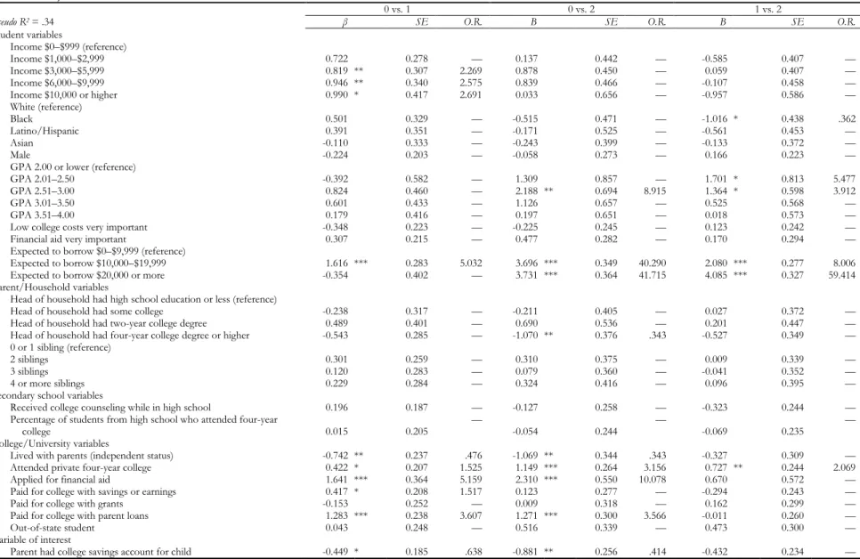
Table 3. Multinomial logistic predicting amount of student loan debt, unadjusted, full model (N = 3,675)

0 vs. 1 0 vs. 2 1 vs. 2

Pseudo R2_{= .34} _β _SE _O.R. _β _SE _O.R. _β _SE _O.R.

Student variables Income $0–$999 (reference) Income $1,000–$2,999 0.316 0.164 — 0.119 0.247 — -0.198 0.232 — Income $3,000–$5,999 0.394 * 0.171 1.484 0.587 * 0.254 1.799 0.193 0.226 — Income $6,000–$9,999 0.304 0.200 — 0.458 0.276 — 0.154 0.262 — Income $10,000 or higher 0.389 0.231 — 0.219 0.353 — -0.169 0.325 — White (reference) Black 0.352 0.193 — -0.370 0.242 — -0.721 ** 0.230 .486 Latino/Hispanic 0.254 0.208 — -0.409 0.313 — -0.664 * 0.277 .515 Asian -0.251 0.205 — -0.268 0.250 — -0.017 0.249 — Male 0.215 0.111 — 0.472 ** 0.169 1.603 0.257 0.142 —

GPA 2.01–2.50 0.394 0.346 — 0.853 0.494 — 0.459 0.408 —

GPA 2.51–3.00 0.699 * 0.285 2.011 1.152 ** 0.375 3.164 0.453 0.330 —

GPA 3.01–3.50 0.400 0.263 — 0.240 0.366 — -0.160 0.318 —

GPA 3.51–4.00 0.042 0.259 — -0.363 0.357 — -0.406 0.318 —

Low college costs very important -0.206 0.150 — -0.274 0.192 — -0.068 0.165 —

Financial aid very important 0.507 * 0.138 1.660 0.704 *** 0.182 2.021 0.197 0.181 —

Expected to borrow $10,000–$19,999 1.696 * 0.186 5.450 3.553 *** 0.219 34.930 1.858 *** 0.164 6.409

Expected to borrow $20,000 or more -0.149 0.232 — 3.552 *** 0.207 34.879 3.701 *** 0.218 40.475

Moderate-income ($35,001–$75,00) 0.168 0.141 — 0.430 * 0.191 1.537 0.262 0.182 —

Middle-income ($75,001–$100,000) -0.140 0.201 — 0.221 0.267 — 0.361 0.231 —

High-income ($100,001 or higher) -0.595 ** 0.198 .552 -0.730 ** 0.280 .482 -0.135 0.270 —

Head of household had some college -0.300 0.218 — -0.044 0.268 — 0.256 0.247 —

Head of household had two-year college degree 0.310 0.262 — 0.531 0.351 — 0.221 0.331 —

Head of household had four-year college degree or higher -0.438 * 0.192 .645 -0.726 ** 0.257 .484 -0.288 0.249 —

2 siblings 0.435 * 0.179 1.545 0.468 0.242 — 0.033 0.219 —

3 siblings 0.220 0.182 — 0.304 0.238 — 0.084 0.229 —

4 or more siblings 0.567 ** 0.198 1.762 0.933 *** 0.265 2.542 0.366 0.244 —

Received college counseling while in high school 0.087 0.115 — -0.162 0.151 — -0.249 0.149 —

Percentage of students from high school who attended four-year college 0.090 0.126 — 0.028 0.159 — -0.063 0.149 —

Lived with parents (independent status) -0.470 ** 0.153 .625 -1.110 *** 0.217 .330 -0.639 ** 0.200 .528

Attended private four-year college 0.249 * 0.123 1.282 0.743 *** 0.178 2.101 0.494 ** 0.163 1.638

Applied for financial aid 1.931 *** 0.221 6.893 1.967 *** 0.355 7.148 0.036 0.394 —

Paid for college with savings or earnings 0.540 *** 0.117 1.716 0.255 0.170 — -0.285 0.155 —

Paid for college with grants 0.130 0.150 — 0.186 0.210 — 0.056 0.201 —

Paid for college with parent loans 0.975 *** 0.135 2.650 1.188 *** 0.175 3.280 0.213 0.168 —

Out-of-state student 0.040 0.144 — 0.240 0.192 — 0.200 0.193 —

Parent had college savings account for child -0.275 * 0.116 .759 -0.633 *** 0.160 .531 -0.358 * 0.146 .699

Note. Data from the Education Longitudinal Study (ELS). β = regression coefficients; SE = standard error; OR = odds ratio. *p < .05; **p < .01; ***p < .001.

(16)

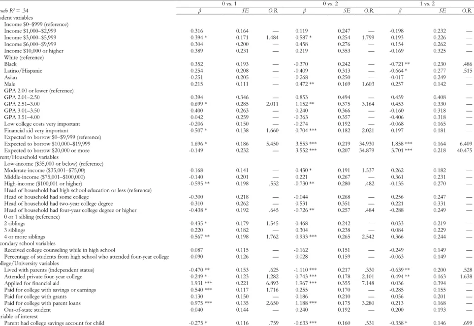
Table 4. Multinomial logistic predicting amount of student loan debt, nearest neighbor matching, full sample (N = 2,661)

0 vs. 1 0 vs. 2 1 vs. 2

Student variables Income $0–$999 (reference) Income $1,000–$2,999 0.150 0.184 — -0.059 0.286 — -0.209 0.280 — Income $3,000–$5,999 0.417 * 0.194 1.518 0.554 * 0.281 1.740 0.137 0.258 — Income $6,000–$9,999 0.141 0.224 — 0.235 0.298 — 0.095 0.311 — Income $10,000 or higher 0.197 0.255 — -0.328 0.417 — -0.525 0.402 — White (reference) Black 0.548 * 0.237 1.730 -0.165 0.300 — -0.713 ** 0.274 .490 Latino/Hispanic 0.347 0.262 — -0.342 0.409 — -0.689 0.353 — Asian -0.265 0.222 — -0.236 0.283 — 0.028 0.277 — Male 0.208 0.128 — 0.403 * 0.199 1.496 0.195 0.175 —

GPA 2.01–2.50 0.558 0.401 — 1.284 * 0.556 3.611 0.726 0.475 —

GPA 2.51–3.00 0.717 * 0.314 2.048 1.194 ** 0.455 3.299 0.476 0.383 —

GPA 3.01–3.50 0.544 0.295 — 0.544 0.438 — 0.000 0.353 —

GPA 3.51–4.00 0.099 0.292 — -0.067 0.429 — -0.166 0.366 —

Low college costs very important -0.338 0.180 — -0.292 0.225 — 0.046 0.200 —

Financial aid very important 0.483 ** 0.153 1.620 0.742 *** 0.205 2.099 0.259 0.205 —

Expected to borrow $10,000–$19,999 1.718 *** 0.226 5.573 3.763 *** 0.269 43.065 2.045 *** 0.205 7.727

Expected to borrow $20,000 or more 0.002 0.261 — 3.724 *** 0.252 41.413 3.722 *** 0.264 41.343

Moderate-income ($35,001–$75,00) 0.149 0.165 — 0.463 * 0.233 1.589 0.314 0.219 —

Middle-income ($75,001–$100,000) -0.202 0.233 — 0.205 0.315 — 0.407 0.277 —

High-income ($100,001 or higher) -0.553 * 0.225 .575 -0.810 * 0.336 .445 -0.257 0.324 —

Head of household had some college -0.638 * 0.275 .528 -0.487 0.348 — 0.152 0.319 —

Head of household had two-year college degree -0.300 0.298 — 0.031 0.423 — 0.330 0.376 —

Head of household had four-year college degree or higher -0.830 *** 0.237 .436 -1.325 *** 0.332 .266 -0.495 0.323 —

2 siblings 0.325 0.199 — 0.282 0.282 — -0.043 0.252 —

3 siblings 0.211 0.203 — 0.291 0.291 — 0.080 0.272 —

4 or more siblings 0.636 ** 0.233 1.888 0.984 ** 0.318 2.676 0.349 0.295 —

Received college counseling while in high school 0.030 0.134 — -0.154 0.184 — -0.184 0.182 —

Percentage of students from high school who attended four-year college 0.012 0.145 — -0.073 0.189 — -0.085 0.175 —

Lived with parents (independent status) -0.293 0.174 — -0.824 ** 0.267 .439 -0.531 * 0.249 .588

Attended private four-year college 0.132 0.141 — 0.637 ** 0.205 1.890 0.504 0.192 —

Paid for college with savings or earnings 0.576 *** 0.131 1.779 0.207 0.185 — -0.369 * 0.178 .691

Paid for college with grants 0.129 0.168 — 0.057 0.251 — -0.072 0.233 —

Out-of-state student 0.064 0.167 — 0.504 * 0.226 1.656 0.440 * 0.224 1.553

Parent had college savings account for child -0.320 * 0.135 .726 -0.778 *** 0.178 .460 -0.457 ** 0.161 .633

Note. Data from the Education Longitudinal Study (ELS). β = regression coefficients; SE = standard error; OR = odds ratio. *p < .05; **p < .01; ***p < .001.

(17)

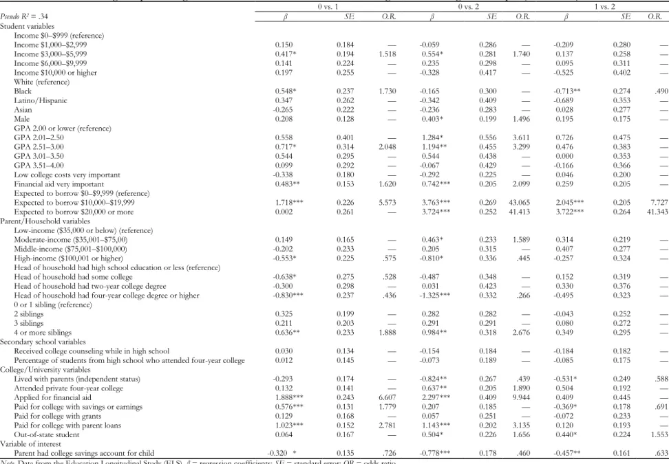
Table 5. Multinomial logistic predicting amount of student loan debt, ATT weighted, full sample (N = 3,675)

0 vs. 1 0 vs. 2 1 vs. 2

Student variables Income $0–$999 (reference) Income $1,000–$2,999 0.223 0.145 — -0.117 0.210 — -0.341 0.202 — Income $3,000–$5,999 0.350 * 0.152 1.418 0.407 0.224 — 0.057 0.204 — Income $6,000–$9,999 0.215 0.185 — 0.283 0.242 — 0.068 0.240 — Income $10,000 or higher 0.344 0.217 — 0.243 0.326 — -0.101 0.293 — White (reference) Black 0.486 * 0.191 1.626 -0.095 0.223 — -0.582 ** 0.207 .559 Latino/Hispanic 0.049 0.203 — -0.328 0.350 — -0.378 0.297 — Asian -0.269 0.162 — -0.493 * 0.231 .611 -0.224 0.239 — Male 0.234 * 0.106 1.264 0.408 ** 0.142 1.504 0.174 0.128 —

GPA 2.01–2.50 0.619 * 0.297 1.857 1.108 ** 0.375 3.028 0.489 0.336 —

GPA 2.51–3.00 0.789 ** 0.250 2.202 0.948 ** 0.334 2.580 0.158 0.293 —

GPA 3.01–3.50 0.400 0.230 — 0.278 0.313 — -0.122 0.271 —

GPA 3.51–4.00 0.116 0.223 — -0.187 0.298 — -0.303 0.269 —

Low college costs very important -0.063 0.138 — -0.165 0.168 — -0.103 0.143 —

Financial aid very important 0.337 ** 0.113 1.401 0.697 *** 0.160 2.008 0.360 * 0.155 1.433

Moderate-income ($35,001–$75,00) 0.196 0.126 — 0.522 ** 0.179 1.685 0.326 0.173 —

Middle-income ($75,001–$100,000) -0.153 0.168 — 0.208 0.228 — 0.360 0.203 —

High-income ($100,001 or higher) -0.553 ** 0.161 0.575 -0.631 * 0.249 .532 -0.078 0.245 —

Head of household had some college -0.270 0.209 — -0.336 0.247 — -0.066 0.215 —

Head of household had four-year college degree or higher -0.408 * 0.189 0.664 -0.805 ** 0.242 0.447 -0.397 0.211 —

2 siblings 0.406 ** 0.153 1.501 0.539 ** 0.203 1.715 0.133 0.194 —

3 siblings 0.325 * 0.165 1.384 0.413 * 0.204 1.511 0.088 0.199 —

4 or more siblings 0.626 ** 0.181 1.869 1.042 *** 0.226 2.836 0.417 0.214 —

Received college counseling while in high school -0.046 0.103 — -0.182 0.140 — -0.135 0.137 —

Percentage of students from high school who attended four-year college -0.068 0.109 — 0.050 0.146 — 0.118 0.136 —

Lived with parents (independent status) -0.184 0.130 — -0.755 *** 0.208 0.470 -0.571 ** 0.195 0.565

Attended private four-year college 0.174 0.107 — 0.677 *** 0.151 1.969 0.503 0.147 —

Applied for financial aid 2.118 *** 0.203 8.313 2.116 *** 0.366 8.295 -0.002 0.397 —

Paid for college with savings or earnings 0.522 *** 0.108 1.686 0.209 0.142 — -0.313 * 0.137 0.731

Paid for college with grants 0.259 * 0.129 1.296 0.258 0.200 — -0.001 0.190 —

Out-of-state student -0.079 0.131 — 0.357 * 0.163 1.430 0.437 ** 0.152 1.548

Parent had college savings account for child -0.176 0.101 — -0.528 *** 0.136 .590 -0.352 ** 0.127 .704

Note. Data from the Education Longitudinal Study (ELS). β = regression coefficients; SE = standard error; OR = odds ratio; ATT = the average treatment effect for the treated using the weight of 1 for a treated case and p/(1-p) for a non-treated case.

(18)

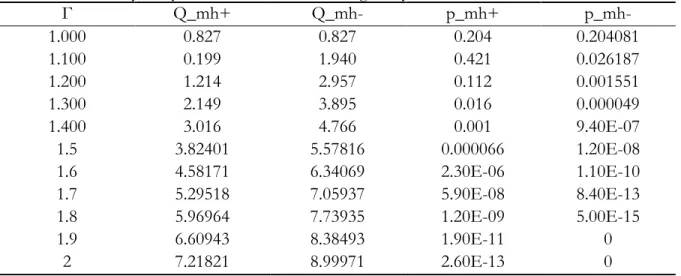
Table 6. Sensitivity analyses for unobserved heterogeneity Γ Q_mh+ Q_mh- p_mh+ p_mh- 1.000 0.827 0.827 0.204 0.204081 1.100 0.199 1.940 0.421 0.026187 1.200 1.214 2.957 0.112 0.001551 1.300 2.149 3.895 0.016 0.000049 1.400 3.016 4.766 0.001 9.40E-07 1.5 3.82401 5.57816 0.000066 1.20E-08 1.6 4.58171 6.34069 2.30E-06 1.10E-10 1.7 5.29518 7.05937 5.90E-08 8.40E-13 1.8 5.96964 7.73935 1.20E-09 5.00E-15 1.9 6.60943 8.38493 1.90E-11 0 2 7.21821 8.99971 2.60E-13 0

Note. Γ = gamma. Q-MH+ = Mantel-Haenszel (1959) statistic for overestimation of treatment effect.

Students with their own incomes of $3,000–$5,999 are about 42% more likely than students with incomes of $0–$999 to have borrowed when all other factors are constant (O.R. = 1.418; p < .05). Black students are 63% more likely than White students to take out small-dollar loans (O.R. = 1.626; p < .05). When contrasted with females, males are about 26% more likely to have borrowed (O.R. = 1.264; p < .05). Contrasted with students with GPAs of 2.00 or lower, those with GPAs between 2.01 and 2.50 are nearly twice as likely to have borrowed (O.R. = 1.857; p < .05), and students with GPAs of 2.51–3.00 are more than twice as likely to have borrowed (O.R. = 2.202; p < .01). Being a student who perceives that the availability of financial aid as very important is associated with being approximately 40% more likely to have borrowed than being a student who does not perceive that the availability of financial aid is very important (O.R. = 1.401; p < .01). Expecting to borrow $10,000–$19,999 rather than $0–$9,999 in the future is associated with students being more than seven times more likely to have borrowed (O.R. = 6.646; p < .001).

The only household variable that increases the likelihood of borrowing is the number of siblings the student has. Contrasted with students who have one or no siblings, those who have two siblings are about 50% more likely to have borrowed (O.R. = 1.501; p < .01), those who have three siblings about 38% more likely to have borrowed (O.R. = 1.384; p < .05), and those who have four siblings or more are nearly twice as likely to have borrowed (O.R. = 1.869; p < .01).

Students who applied for financial aid versus students who did not are eight times more likely to have borrowed (O.R. = 8.313; p < .001). Students who paid for college with their own savings or earnings are 69% more likely to have borrowed than students who did not pay for college with their own savings or earnings (O.R. = 1.686; p < .001). Students who paid for college with grants are 30% more likely to have borrowed than students who did not pay for college with grants (O.R. = 1.296; p < .05). Students who paid for college with parents’ loans are about three times more likely to have borrowed than students with parents who did not pay for college with parents’ loans (O.R. = 2.741; p < .001).

We also find two household variables that are negative significant predictors of the amount of student loan debt: living in a high-income household and having parents with four-year degrees or higher. Negative predictors decrease the chance that a student borrows between $0 and $9,999.

(19)

Household income works as a protective factor against borrowing. Contrasted with low-income students, high-income students are about 42% less likely to have borrowed (O.R. = 0.575; p < .01). Contrasted with students whose parents have a high school education or less, students with parents who have four years of college or more are about 34% less likely to have borrowed (O.R. = 0.664; p < .05).

Multinomial logistic results for high-dollar student loans ($10,000 or higher) relative to not borrowing, full sample

We find that positive significant predictors of high-dollar loans include gender, GPA, having reported financial aid as very important, amount expected to borrow, income, number of siblings, attendance at a private four-year college, having applied for financial aid, having paid for college with parents’ loans, and having attending college out of state (see Table 5).

Contrasted with females, males are about 50% more likely to have borrowed (O.R. = 1.504; p < .001). Contrasted with students who have GPAs of 2.00 or lower, those with GPAs between 2.01 and 2.50 are about three times more likely to have borrowed (O.R. = 3.028; p < .01), and those with GPAs between 2.51 and 3.00 are more than two and half times more likely to have borrowed (O.R. = 2.580; p < .01). Students who perceive the availability of financial aid as very important are more than twice as likely to have borrowed than students who did not perceive the availability of financial aid is very important (O.R. = 2.008; p < .01). Contrasted with students who expected to borrow $0–$9,999, those who expected to borrow $10,000–$19,999 are more than 40 times more likely to have borrowed (O.R. = 40.305; p < .001), and those who expected to borrow $20,000 or more are more than 36 times more likely to have borrowed (O.R. = 36.337; p < .001). Surprisingly, contrasted with low-income students, moderate-income students are about 69% more likely to have borrowed (O.R. = 1.685; p < .01).

The only household variable that increases the likelihood of borrowing $10,000 or more is the number of siblings the student has. Contrasted with students who have one or no siblings, those who have two siblings are about 72% more likely to have borrowed (O.R. = 1.715; p < .01), those who have three siblings are about 51% more likely to have borrowed (O.R. = 1.511; p < .05), and those who have four siblings or more are nearly three times more likely to have borrowed (O.R. = 2.836; p < .01).

Contrasted with students who attended public year colleges, those who attended private four-year colleges are twice as likely to have borrowed (O.R. = 1.969; p < .001). Students who applied for financial aid are about eight times more likely to have borrowed than students who did not apply for financial aid (O.R. = 8.295; p < .001). Students who paid for college with parents’ loans are about three times more likely to have borrowed than students who did not pay for college with parents’ loans (O.R. = 3.109; p < .001). Out-of-state students are about 43% more likely to have borrowed than in-state students (O.R. = 1.430; p < .05).

We also find that race, income, parent’s level of education, having lived with parents, and parents’ college savings accounts are negative significant predictors of amount of student loan debt.

Contrasted with White students, Asian students are 39% less likely to have borrowed (O.R. = 0.611; p < .05). Contrasted with students in low-income households, those in high-income households are 47% less likely to have borrowed (O.R. = 0.532; p < .05). Contrasted with students whose parents had a high school education or less, students whose parents had some college are about 55% less

(20)

likely to have borrowed (O.R. = 0.447; p < .001). Contrasted with students who lived on their own, those who lived with parents are 53% less likely to borrow (O.R. = 0.470; p < .001).

Regarding our variable of interest—whether or not parents had college savings accounts—students whose parents had college savings accounts are 41% less likely to have borrowed than students whose parents did not have college savings accounts (O.R. = 0.590; p < .001).

Results by Income Level

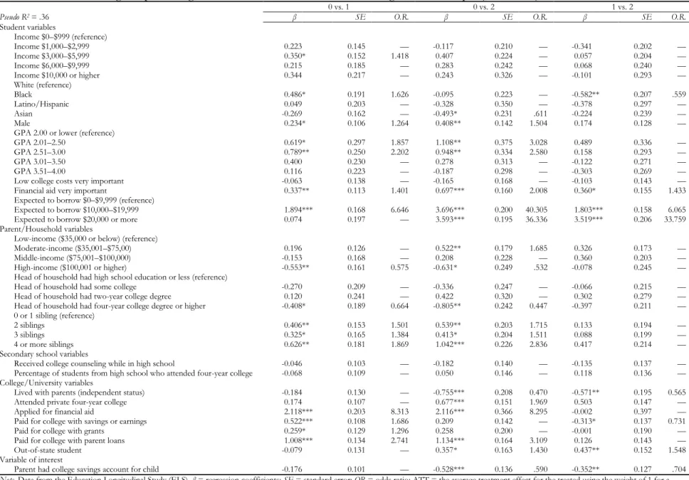
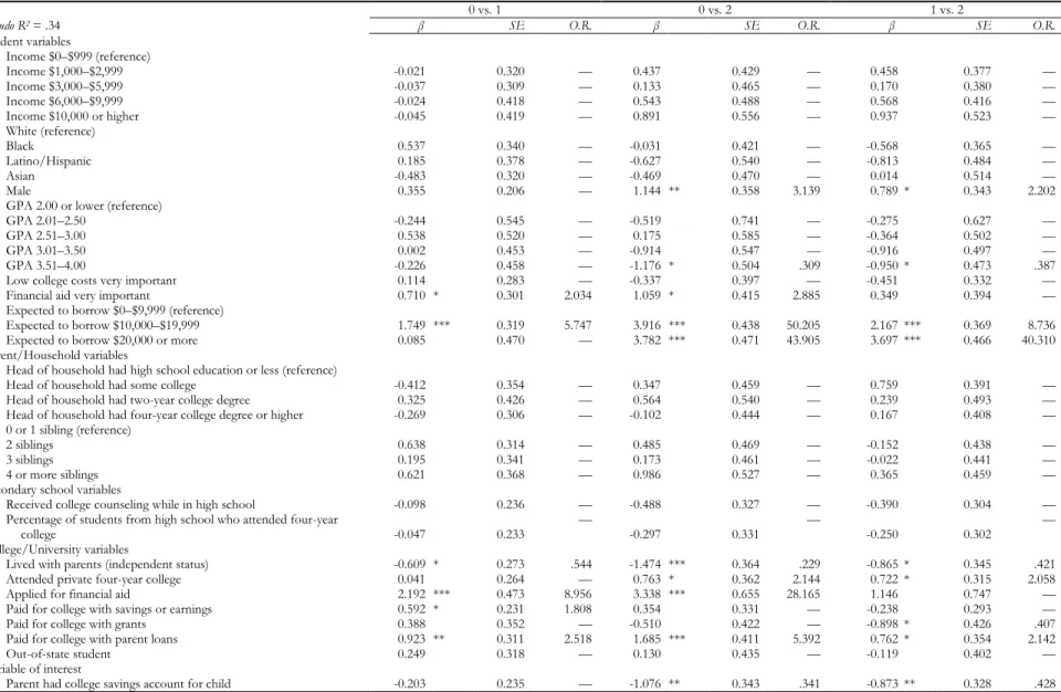
Multinomial logistic results for small-dollar student loans ($0–$9,999) relative to not borrowing, low-income ($35,000 or below) sample

Results from multinomial logistic regression predicting amount of student loan debt are reported in Tables 7 and 8. We find that positive significant predictors include race, gender, having reported financial aid as very important, amount expected to borrow, having applied for financial aid, having paid for college with savings or earnings, and having paid for college with parents’ loans.

Contrasted with White students, Black students are more than three times more likely to have borrowed than not (O.R. = 3.223; p < .01). Contrasted with females, males are about 65% more likely to have borrowed (O.R. = 1.654; p < .05). Students who perceived the availability of financial aid as very important are more than twice as likely to have borrowed than students who did not perceive that availability of financial aid is very important (O.R. = 2.390; p < .01). Contrasted with students who expected to borrow $0–$9,999, those who expected to borrow $10,000–$19,999 are more than six times more likely to have borrowed (O.R. = 5.955; p < .001), and those who expected to borrow $20,000 or more are more than three times more likely to have borrowed (O.R. = 3.072; p < .05).

Several college or university factors increase students’ likelihood of borrowing. Students who applied for financial aid are about ten times more likely to have borrowed than students who did not apply for financial aid (O.R. = 9.860; p < .001). Students who paid for college with their own savings or earnings are 77% more likely to have borrowed than students who did not pay for college with their own savings or earnings (O.R. = 1.772; p < .05). Students who paid for college with parents’ loans are about three times more likely to have borrowed than students who did not pay for college with parents’ loans (O.R. = 2.953; p < .01).

We also find the only negative significant predictor of amount of student loan debt is having lived in a household with parents who have some college. Contrasted with students whose parents had a high school education or less, those whose parents had some college are about 53% less likely to have borrowed (O.R. = 0.468; p < .05).

Multinomial logistic results for high-dollar student loans ($10,000 or higher) relative to not borrowing, low-income ($35,000 or below) sample

We find that positive significant predictors of amount of student loan debt include gender, GPA, having reported financial aid as very important, amount expected to borrow, having attended a private four-year college, having applied for financial aid, having paid for college with parents’ loans, and having attended college out of state (see Table 7).

(21)

Table 7. Multinomial logistic regression predicting amount of student loan debt, unadjusted, low-income ($35,000 or below) sample (N = 860)

0 vs. 1 0 vs. 2 1 vs. 2

Student variables Income $0–$999 (reference) Income $1,000–$2,999 -0.021 0.320 — 0.437 0.429 — 0.458 0.377 — Income $3,000–$5,999 -0.037 0.309 — 0.133 0.465 — 0.170 0.380 — Income $6,000–$9,999 -0.024 0.418 — 0.543 0.488 — 0.568 0.416 — Income $10,000 or higher -0.045 0.419 — 0.891 0.556 — 0.937 0.523 — White (reference) Black 0.537 0.340 — -0.031 0.421 — -0.568 0.365 — Latino/Hispanic 0.185 0.378 — -0.627 0.540 — -0.813 0.484 — Asian -0.483 0.320 — -0.469 0.470 — 0.014 0.514 — Male 0.355 0.206 — 1.144 ** 0.358 3.139 0.789 * 0.343 2.202

GPA 2.01–2.50 -0.244 0.545 — -0.519 0.741 — -0.275 0.627 —

GPA 2.51–3.00 0.538 0.520 — 0.175 0.585 — -0.364 0.502 —

GPA 3.01–3.50 0.002 0.453 — -0.914 0.547 — -0.916 0.497 —

GPA 3.51–4.00 -0.226 0.458 — -1.176 * 0.504 .309 -0.950 * 0.473 .387

Low college costs very important 0.114 0.283 — -0.337 0.397 — -0.451 0.332 —

Financial aid very important 0.710 * 0.301 2.034 1.059 * 0.415 2.885 0.349 0.394 —

Head of household had some college -0.412 0.354 — 0.347 0.459 — 0.759 0.391 —

Head of household had four-year college degree or higher -0.269 0.306 — -0.102 0.444 — 0.167 0.408 —

2 siblings 0.638 0.314 — 0.485 0.469 — -0.152 0.438 —

3 siblings 0.195 0.341 — 0.173 0.461 — -0.022 0.441 —

4 or more siblings 0.621 0.368 — 0.986 0.527 — 0.365 0.459 —

Percentage of students from high school who attended four-year

college -0.047 0.233 — -0.297 0.331 — -0.250 0.302 —

Lived with parents (independent status) -0.609 * 0.273 .544 -1.474 *** 0.364 .229 -0.865 * 0.345 .421

Attended private four-year college 0.041 0.264 — 0.763 * 0.362 2.144 0.722 * 0.315 2.058

Paid for college with savings or earnings 0.592 * 0.231 1.808 0.354 0.331 — -0.238 0.293 —

Paid for college with grants 0.388 0.352 — -0.510 0.422 — -0.898 * 0.426 .407

Paid for college with parent loans 0.923 ** 0.311 2.518 1.685 *** 0.411 5.392 0.762 * 0.354 2.142

Out-of-state student 0.249 0.318 — 0.130 0.435 — -0.119 0.402 —

Parent had college savings account for child -0.203 0.235 — -1.076 ** 0.343 .341 -0.873 ** 0.328 .428

(22)

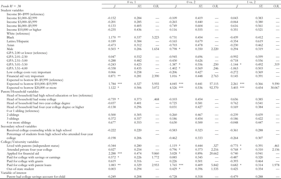
Table 8. Multinomial logistic regression predicting amount of student loan debt, ATT weighted, low-income ($35,000 or below) sample (N = 860)

0 vs. 1 0 vs. 2 1 vs. 2

Student variables Income $0–$999 (reference) Income $1,000–$2,999 -0.152 0.284 — -0.109 0.419 — 0.043 0.383 — Income $3,000–$5,999 -0.201 0.285 — -0.265 0.440 — -0.064 0.380 — Income $6,000–$9,999 0.133 0.405 — 0.749 0.604 — 0.616 0.561 — Income $10,000 or higher -0.235 0.436 — 0.116 0.555 — 0.351 0.521 — White (reference) Black 1.170 ** 0.337 3.223 0.731 0.454 — -0.439 0.412 — Latino/Hispanic 0.189 0.384 — -0.165 0.679 — -0.354 0.619 — Asian -0.473 0.312 — -0.703 0.478 — -0.230 0.462 — Male 0.503 * 0.206 1.654 0.798 * 0.350 2.220 0.294 0.319 —

GPA 2.01–2.50 0.047 0.552 — -0.945 0.696 — -0.992 0.599 —

GPA 2.51–3.00 0.288 0.482 — -0.430 0.626 — -0.718 0.556 —

GPA 3.01–3.50 -0.243 0.423 — -1.387 * 0.556 .250 -1.144 * 0.492 .319

GPA 3.51–4.00 -0.338 0.435 — -1.402 * 0.569 .246 -1.063 0.503 —

Low college costs very important 0.066 0.258 — -0.206 0.427 — -0.272 0.369 —

Financial aid very important 0.871 ** 0.281 2.390 1.016 * 0.448 2.763 0.145 0.391 —

Expected to borrow $20,000 or more 1.122 * 0.506 3.072 4.526 *** 0.536 92.370 3.403 *** 0.454 30.067

Head of household had some college -0.759 * 0.373 .468 -0.103 0.454 — 0.656 0.385 —

Head of household had two-year college degree -0.037 0.401 — 0.725 0.581 — 0.762 0.541 —

Head of household had four-year college degree or higher -0.138 0.296 — 0.031 0.427 — 0.169 0.384 —

2 siblings 0.500 0.305 — 0.260 0.467 — -0.239 0.439 —

3 siblings 0.372 0.357 — 0.186 0.454 — -0.186 0.422 —

4 or more siblings 0.677 0.353 — 0.630 0.500 — -0.048 0.447 —

Percentage of students from high school who attended four-year

college -0.198 0.206 — -0.462 0.333 — -0.264 0.307 —

Lived with parents (independent status) -0.344 0.280 — -1.119 * 0.444 .327 -0.775 * 0.391 .461

Attended private four-year college 0.027 0.254 — 0.796 * 0.373 2.216 0.768 * 0.310 2.156

Applied for financial aid 2.288 *** 0.474 9.860 3.028 * 0.896 20.662 0.740 0.941 —

Paid for college with savings or earnings 0.572 * 0.226 1.772 0.085 0.345 — -0.487 0.320 —

Paid for college with grants 0.619 0.316 — 0.226 0.501 — -0.393 0.464 —

Paid for college with parent loans 1.083 ** 0.329 2.953 1.765 *** 0.409 5.842 0.682 * 0.314 1.978

Out-of-state student 0.003 0.294 — 0.429 * 0.396 1.535 0.425 0.354 —

Parent had college savings account for child -0.249 0.208 — -0.728 0.318 — -0.479 0.288 —