Daniel Paravisini
, Veronica Rappoport, Enrichetta Ravina
Risk aversion and wealth: evidence from
person-to-person lending portfolios
Article (Accepted version)
(Refereed)
Original citation:
Paravisini, Daniel, Rappoport, Veronica and Ravina, Enrichetta (2016) Risk aversion and wealth: evidence from person-to-person lending portfolios.Management Science. ISSN 0025-1909
DOI: 10.1287/mnsc.2015.2317
© 2016 INFORMS
This version available at: http://eprints.lse.ac.uk/62137/
Available in LSE Research Online: November 2016
LSE has developed LSE Research Online so that users may access research output of the School. Copyright © and Moral Rights for the papers on this site are retained by the individual authors and/or other copyright owners. Users may download and/or print one copy of any article(s) in LSE Research Online to facilitate their private study or for non-commercial research. You may not engage in further distribution of the material or use it for any profit-making activities or any commercial gain. You may freely distribute the URL (http://eprints.lse.ac.uk) of the LSE Research Online website.
This document is the author’s final accepted version of the journal article. There may be differences between this version and the published version. You are advised to consult the publisher’s version if you wish to cite from it.
Risk Aversion and Wealth:
Evidence from Person-to-Person Lending Portfolios
∗Daniel Paravisini Veronica Rappoport Enrichetta Ravina
LSE, BREAD, CEPR LSE, CEP, CEPR Columbia GSB
August 10, 2015
Abstract
We estimate risk aversion from investors’ financial decisions in a person-to-person lending plat-form. We develop a method that obtains a risk aversion parameter from each portfolio choice. Since the same individuals invest repeatedly, we construct a panel dataset that we use to disen-tangle heterogeneity in attitudes towards risk across investors, from the elasticity of risk aversion to changes in wealth. We find that wealthier investors are more risk averse in the cross section, and that investors become more risk averse after a negative housing wealth shock. Thus, in-vestors exhibit preferences consistent with decreasing relative risk aversion and habit formation. JEL codes: E21, G11, D12, D14.
∗
We are grateful to Lending Club for providing the data and for helpful discussions on this project. We thank Michael Adler, Manuel Arellano, Nick Barberis, Geert Bekaert, Patrick Bolton, John Campbell, Marco di Maggio, Larry Glosten, Nagpurnanand Prabhala, Bernard Salanie, and seminar participants at CEMFI, Columbia University GSB, Duke Fuqua School of Business, Hebrew University, Harvard Business School, Kellogg School of Manage-ment, Kellstadt Graduate School of Business-DePaul, London Business School, Maryland Smith School of Busi-ness, M.I.T. Sloan, Universidad Nova de Lisboa, the Yale 2010 Behavioral Science Conference, and the SED 2010 meeting for helpful comments. We thank the Program for Financial Studies for financial support. All remaining errors are our own. Please send correspondence to Daniel Paravisini (d.paravisini@lse.ac.uk), Veronica Rappoport (v.e.rappoport@lse.ac.uk), and Enrichetta Ravina (er2463@columbia.edu).
1
Introduction
Theoretical predictions on investment, asset prices, and the cost of business cycles depend crucially on assumptions about the relationship between risk aversion and wealth.1 Although characterizing
this relationship has long been in the research agenda of empirical finance and economics, progress has been hindered by the difficulty of disentangling the shape of the utility function from preference heterogeneity across agents. For example, the bulk of existing work is based on comparisons of risk aversion across investors of different wealth, which requires assuming that agents have the same
preference function. If agents have heterogeneous preferences, however, cross sectional analysis leads to incorrect inferences about the shape of the utility function when wealth and preferences are correlated. Such a correlation may arise, for example, if agents with heterogeneous propensity to take risk make different investment choices, which in turn affect their wealth.2 To both characterize the properties of the joint distribution of preferences and wealth in the cross section, and estimate the parameters describing the utility function, one needs to observe how the risk aversion of the same individual changes with wealth shocks.
Important recent work improves on the cross-sectional approach by looking at changes in the fraction of risky assets in an investor’s portfolio stemming from the time series variation in investor wealth.3 The crucial identifying assumption required for using the share of risky assets as a proxy for investor Relative Risk Aversion (RRA) in this setting is that all other determinants of the share of risky assets remain constant as the investor’s wealth changes. One must assume, for example, that changes in financial wealth resulting from the performance of risky assets are uncorrelated with changes in beliefs about their expected return and risk. Attempts to address this identification problem through an instrumental variable approach have produced mixed results: the estimated sign of the elasticity of RRA to wealth varies across studies depending on the choice of instrument.4
1
See Kocherlakota (1996) for a discussion of the literature aiming at resolving theequity premiumandlow risk free
rate puzzles under different preference assumptions. Following the seminal contribution in Campbell and Cochrane
(1999), recent work shows that preferences with habit formation produce cyclical variations in risk aversion and decreasing relative risk aversion after a positive wealth shock that can explain these and other empirical asset pricing regularities (Menzly et al., 2004, Buraschi and Jiltsov, 2007, Polkovnichenko, 2007, Yogo, 2008, Korniotis, 2008, and Santos and Veronesi, 2010). Wealth inequality has also been shown to raise the equity premium if the absolute risk aversion is concave in wealth (Gollier, 2001).
2
Guvenen (2009) and Gomes and Michaelides (2008) propose a model with preference heterogeneity that endoge-nously generates cross sectional variation in wealth. Alternatively, an unobserved investor characteristic, such as having more educated parents, may jointly affect wealth and the propensity to take risk.
3Chiappori and Paiella (2011), Brunnermeier and Nagel (2008), and Calvet et al. (2009).
4
Finally, estimates of risk aversion based on the share of risky assets pose an additional problem when used to analyze the link between heterogeneity in risk preferences and wealth: measurement error in wealth is inherited by the risk aversion estimates, and may induce a spurious correlation between the two. This potentially explains why existing empirical evidence on the correlation between risk preferences and wealth in the cross section is inconclusive, depends on the definition of wealth, and is sensitive to the categorization of assets into the risky and riskless categories.5
The present paper exploits a novel environment to obtain, independently of wealth, unbiased measures of investor risk aversion and to examine the link between these estimates and investor wealth. We analyze the risk taking behavior of 2,372 investors based on their actual financial decisions in Lending Club (LC), a person-to-person lending platform in which individuals invest in diversified portfolios of small loans.6 We develop a methodology to estimate the local curvature of an investor’s utility function (Absolute Risk Aversion, or ARA) from each portfolio choice. The key advantage of this estimation approach is that it does not require characterizing investors’ outside wealth. We also exploit the fact that the same individuals make repeated investments in LC to construct a panel of risk aversion estimates. We use this panel to both characterize the cross sectional correlation between risk preferences and wealth, and to obtain reduced form estimates of the elasticity of investor-specific risk aversion to changes in wealth. We find the cross-sectional elasticity between Relative Risk Aversion (RRA) and wealth to be positive, and the investor-specific wealth elasticities to be negative.
Our estimation method is derived from an optimal portfolio model where investors hold an unknown number of risky and riskless assets, including a portfolio of LC loans. We decompose the LC returns into a systematic component and an idiosyncratic return component orthogonal to the market. We use the idiosyncratic component to characterize investors’ preferences: an investor’s ARA is given by the additional expected return that makes her indifferent about allocating the marginal dollar to a loan with higher idiosyncratic default probability. Estimating risk preferences from the non-systematic component of returns implies that the estimates are independent from the investors’ overall risk exposure or wealth. Moreover, by measuring the curvature of the utility function directly from the first order condition of this portfolio choice problem, we do not need to
5
See, among others, Blume and Friend (1975), Cohn et al. (1975), Morin and Suarez (1983), and Blake (1996).
6For prior research analyzing investors’ behavior in peer-to-peer lending see Iyer et al. (2014) , Lin et al. (2013),
impose a specific shape of the utility function.
This method relies on two assumptions that we validate in the data. The first assumption is that LC loans are not held to simply replicate the market portfolio. This assumption is validated by the substantial heterogeneity of mean and variance across investors’ LC portfolios. The second assumption is that we can correctly capture investors’ beliefs about the stochastic distribution of returns using the information provided on the LC’s web site. Although we cannot observe the investors’ beliefs, we test this assumption indirectly by exploiting a feature of the LC environment: Many investors choose LC loans both manually and through an optimization tool based on returns and default probabilities posted on the LC site. We use the sample of investors that use both methods to show that our estimate of investor-specific risk aversion obtained from the manually chosen component of their LC portfolio does not differ significantly from the estimate obtained from the component of the portfolio chosen with the tool. Testing the validity of assumptions concerning person-specific priors on idiosyncratic risk is typically impossible in real-life environments. Being able to validate our assumptions, although in an admittedly indirect way, represents an important advantage of this setting.
With this method we estimate parameters of risk aversion for each investor and portfolio choice in our sample. The average ARA implied by the tradeoff between expected return and idiosyncratic risk in our sample of portfolio choices is 0.037. Our estimates imply an average income-based Relative Risk Aversion (income-based RRA) of 2.81, with substantial unexplained heterogeneity and skewness.7
In estimating risk attitudes based on idiosyncratic risk, our approach is similar to that of the economic literature that studies risk attitudes and insurance choices (Cohen and Einav, 2007; Barseghyan et al., 2013; Einav et al., 2012). Our estimates are also comparable to experimental measures of risk aversion, as investors in our model face choices similar to those faced by experimen-tal subjects along important dimensions. Our model transforms a complex portfolio choice problem into a choice between well-defined lotteries of pure idiosyncratic risk, where returns are character-ized by a discrete failure probability (i.e., default), and the stakes are small relative to total wealth (the median investment in LC is $375).8 The level, distribution, and skewness of the estimated
7
The income-based RRA is a risk preference parameter often reported in the experimental literature. It is obtained
assuming that the investor’s outside wealth is zero; that is: ARA·E[y], whereE[y] is the expected income from the
lottery offered in the experiment.
8
risk aversion parameters are similar to those obtained in laboratory and field experiments.9 These similarities indicate that investors in our sample, despite being a self-selected sample of individuals who invest on-line, have risk preferences similar to individuals in other settings.
We show that our method generates consistent estimates for the curvature of the utility function under the expected utility framework and alternative preference specifications, such as loss aversion and narrow framing, as in Barberis and Huang (2001) and Barberis et al. (2006). This is a key feature of our estimation procedure since under the expected utility framework the observed high levels of risk aversion in small stake environments are difficult to reconcile with the observable be-havior of agents in environments with larger stakes (Rabin, 2000). We also show that our estimates of the elasticity of ARA with respect to investor’s wealth characterize agents’ risk attitudes, both, in large and small stake environments.
We exploit the panel dimension of our data to derive the cross-sectional and within-investor elasticities of risk aversion with respect to wealth. First, in the cross section, we find that wealthier investors exhibit lower ARA and higher RRA. Since we use imputed net worth as a proxy for wealth, our preferred specification corrects for measurement error in the wealth proxy using house prices in the investor’s zip code as an instrument. We obtain an elasticity of ARA to wealth of -0.074, which implies a cross sectional wealth elasticity of the RRA of 0.93.10 These findings coincide qualitatively with Guiso and Paiella (2008) and Cicchetti and Dubin (1994), who also base their analysis on risk aversion parameters estimated independently of their wealth measure.
Second, we estimate the elasticity of risk aversion to changes in wealth in an investor fixed-effect specification to characterize the shape of the utility function for the average investor. We use the decline in house prices in the investor’s zip code during our sample period—October 2007 to April 2008—as a source of variation in investor wealth. The results indicate that the average investor’s RRA increases after experiencing a negative housing wealth shock, with an estimated elasticity of −1.85. This is consistent with investors exhibiting decreasing Relative Risk Aversion, and with theories of habit formation (as in Campbell and Cochrane, 1999) and incomplete markets (as in
Jullien and Salanie (2008), Bombardini and Trebbi (2012), Harrison, Lau and Towe (2007), Chiappori et al. (2008), Post et al. (2008), Chiappori et al. (2009), and Barseghyan et al. (2011).
9
See for example Barsky et al. (1997), Holt and Laury (2002), Choi et al. (2007), and Harrison, Lau and Rutstrom (2007).
10
The wealth-based RRA is not directly observable, we compute its elasticity from the following relationship:
Guvenen, 2009).11
The contrasting signs of the cross-sectional and within-investor elasticities confirm that investors have heterogeneous risk preferences that are correlated with wealth in the cross section. This implies that inference on the elasticity of risk aversion to wealth from cross sectional data will be biased. In our setting, the bias implied by the joint distribution of preferences and wealth is large enough to flip the sign of the investor-specific risk aversion elasticity to wealth.12
A novel feature of our estimation approach is that it disentangles the measurement of risk aversion from investors’ assessments about the systematic risk of LC loans. On average, investors’ perceived systematic risk premium in LC increases from 5.7% to 8.9% between the first and last months of the sample period. The increase in the perceived systematic risk is concurrent with the drop in house prices, which indicates that wealth shocks are potentially correlated with general changes in investors’ beliefs. This calls for caution when using the share of risky assets as a measure of investor RRA. In our context, inference based on the share of risky assets alone would have led us to overestimate the investor-specific elasticity of risk aversion to wealth.
The rest of the paper is organized as follows. Section 2 describes the Lending Club platform. Section 3 illustrates the portfolio choice model and sets out our estimation strategy. Section 4 describes the data and the sample restrictions. Section 5 presents and discusses the empirical results and provides a test of the identification assumptions. Section 6 explores the relationship between risk preferences and wealth. And Section 7 concludes.
2
The Lending Platform
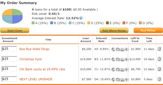
Lending Club (LC) is an online U.S. lending platform that allows individuals to invest in portfolios of small loans. The platform started operating in June 2007. As of May 2010, it has funded $112,003,250 in loans and provided an average net annualized return of 9.64% to investors.13 Below,
11These preference specifications are also consistent with the empirical findings in Calvet et al. (2009). Brunnermeier
and Nagel (2008), on the other hand, find support for CRRA.
12Chiappori and Paiella (2011) find the bias from the cross sectional estimation to be economically insignificant
when risk aversion is measured using the share of risky assets. Tanaka et al. (2010) use rainfall across villages in Vietnam as an instrument for wealth in the cross section and find significant difference between the OLS and IV estimators. However, to obtain the elasticity of the agent-specific risk aversion, they must assume that preferences are equal across villages otherwise.
13The median investor in our sample period is a retail investor. The composition then shifted towards institutional
investors, a common trend in the peer-to-peer industry. As of 2014, 80% of investment going into P2P platforms
we provide an overview of the platform and derive the expected return and variance of investors’ portfolio choices.
2.1 Overview
Borrowers need a U.S. SSN and a FICO score of 640 or higher in order to apply. They can request a sum ranging from $1,000 to $25,000, usually to consolidate credit card debt, finance a small business, or fund educational expenses, home improvements, or the purchase of a car.
Each application is classified into one of 35 risk buckets based on the FICO score, the requested loan amount, the number of recent credit inquiries, the length of the credit history, the total and currently open credit accounts, and the revolving credit utilization, according to a pre-specified published rule posted on the website.14 LC also posts a default rate for each risk bucket, taken from a long term validation study by TransUnion, based on U.S. unsecured consumer loans. All the loans classified in a given bucket offer the same interest rate, assigned by LC based on an internal rule.
A loan application is posted on the website for a maximum of 14 days. It becomes a loan only if it attracts enough investors and gets fully funded. All the loans have a 3 year term with fixed interest rates and equal monthly installments, and can be prepaid with no penalty for the borrower. When the loan is granted, the borrower pays a one-time fee to LC ranging from 1.25% to 3.75%, depending on the risk bucket. When a loan repayment is more than 15 days late, the borrower is charged a late fee that is passed to investors. Loans with repayments more than 120 days late are considered in default, and LC begins the collection procedure. If collection is successful, investors receive the amount repaid minus a collection fee that varies depending on the age of the loan and the circumstances of the collection. Borrower descriptive statistics are shown in Table 1, panel A. Investors in LC allocate funds to open loan applications. The minimum investment in a loan is $25. According to a survey of 1,103 LC investors in March 2009, diversification and high returns relative to alternative investment opportunities are the main motivations for investing in LC.15LC
refer to: https://www.lendingclub.com/info/statistics.action.
14Please refer to https://www.lendingclub.com/info/how-we-set-interest-rates.action for the details of the
classifi-cation rule and for an example.
15To the question “What would you say was the main reason why you joined Lending Club”, 20% of respondents
replied “to diversify my investments”, 54% replied “to earn a better return than (...)”, 16% replied “to learn more about peer lending”, and 5% replied “to help others”. In addition, 62% of respondents also chose diversification and higher returns as their secondary reason for joining Lending Club.
lowers the cost of investment diversification inside LC by providing an optimization tool that con-structs the set of efficient loan portfolios for the investor’s overall amount invested in LC—i.e., the minimum idiosyncratic variance for each level of expected return (see Figure 1).16 In other words, the tool helps investors to process the information on interest rates and default probabilities posted on the website into measures of expected return and idiosyncratic variance, that may otherwise be difficult to compute for an average investor (these computations are performed in Subsection 2.2).17 When investors use the tool, they select, among all the efficient portfolios, the preferred one according to their own risk preferences. Investors can also use the tool’s recommendation as a starting point and then make changes. Or they can simply select the loans in their portfolio manually.
Of all portfolio allocations between LC’s inception and June 2009, 39.6% was suggested by the optimization tool, 47.1% was initially suggested by the tool and then altered by the investor, and the remaining 13.3% was chosen manually.18
Given two loans that belong to the same risk bucket (with the same idiosyncratic risk), the optimization tool suggests the one with the highest fraction of the requested amount that is already funded. This tie-breaking rule maximizes the likelihood that loans chosen by investors are fully funded. In addition, if a loan is partially funded at the time the application expires, LC provides the remaining funds.
2.2 Return and Variance of the Risk Buckets
This subsection derives the expected return and variance of individual loans and risk buckets, following the same assumptions as the LC platform. All the loans in a given risk bucketz= 1, ...,35 are characterized by the same scheduled monthly payment per dollar borrowed,Pz, over the 3 years
(36 monthly installments). The per dollar scheduled payment Pz and the bucket specific default
rate πz fully characterize the expected return and variance ofper project investments, µz and σz2.
LC considers a geometric distribution for the idiosyncratic monthly survival probability of the
16
During the period analyzed in this paper, the portfolio tool appeared as the first page to the investors. LC has recently changed its interface and, before the portfolio tool page, it has added a stage where the lender can simply pick between 3 representative portfolios of different risk and return.
17The tool normalizes the idiosyncratic variance into a 1–0 scale. Thus, while the tool provides an intuitive sorting
of efficient portfolios in terms of their idiosyncratic risk, investors always need to analyze the recommended portfolios of loans to understand the actual risk level imbedded in the suggestion.
18
individual projects: The probability that the loan survives until monthτ ∈[1,36] is Pr (T =τ) = πz(1−πz)τ.19 The resulting expectation and variance of the present value of the payments,Pz, of
any project in bucketz are:
µz = Pz " 1− 1−πz 1 +r 36# 1−πz r+πz σz2 = 35 X t=1 πz(1−πz)t t X τ=1 Pz (1 +r)τ !2 + 36 X τ=1 Pz (1 +r)τ !2 (1−πz)36−µ2z
wherer is the risk-free interest rate.
The idiosyncratic risk associated with bucketzdecreases with the level of diversification within the bucket; that is, the number of projects from bucket z in the portfolio of investor i, niz. The resulting idiosyncratic variance is therefore investor specific:
varrzi= σ 2 z ni z . (1)
whereriz is the idiosyncratic component of the bucket’s return,Riz
Then, the variance of the return on investment in bucket z can be decomposed as follows:
var Riz =Vzi+σ 2 z ni z
whereVzicorresponds to the bucket’s non-diversifiable risk andσz2/nizis its idiosyncratic component. The expected return of an investment in bucketz is not affected by the number of loans in the investor’s portfolio; it is equal to the expected return on a loan in bucket z, µz, and is constant
across investors:20 E[Rz] =E Riz =µz. (2) 19
Although LC does not explicitly state in the web page that the probabilities of default are idiosyncratic, the optimization tool used to calculate the set of minimum variance portfolios works under this assumption.
20
The analysis in subsection 5.2 confirms that investors’ beliefs about the probabilities of default do not differ
3
Estimation Procedure
To capture the fact that most individuals invest not only in the market and the risk free asset but also in individual securities, our framework considers investors that, instead of simply holding a replica of the market portfolio, also hold securities based on their own subjectiveinsights that they will generate an excess return. The decision to invest in LC depends on investors’ knowledge of its existence and their subjective expectation that LC is, indeed, a good investment opportunity. Thus, it is reasonable to assume that investors in LC have special insights, which explains why, as we show later, their portfolio departs from just replicating the market.21
Our framework starts by recognizing that there is a high degree of comovement between se-curities, and specifically to our case, the probability of default of the loans in LC is potentially correlated with macroeconomic fluctuations. We use the Sharpe Diagonal Model to capture this feature and assume that returns are related only through a common systematic factor (i.e., market or macroeconomic fluctuations). Under this assumption, returns on LC loans can be decomposed into a common systematic factor and a component orthogonal to the market (we also refer to it as
independent component).
The advantage of this model is that the optimal portfolio of LC loans depends only on the expected return and variance of the independent component, as the next subsection shows. In other words, the optimal amount invested in each LC bucket does not depend on the return covariance with the investor’s overall risk exposure, nor does it require knowing the amount and characteristics of her outside wealth.
We test the assumptions on investors’ beliefs in Section 5, i.e. that they act as if there is a common systematic factor, and that the choice of LC loans does not simply replicate the market portfolio. The data strongly support both hypotheses.
3.1 The Model
Each investorichooses the share of wealth to be invested in z= 1, ..., Z securities with returnRz
andZ ≥35. We consider securitiesz= 1, ...,35 to represent the LC risk buckets. And we explicitly include outside investment options, z= 36, ..., Z, that represent the market composite, a risk-free asset, real estate, human capital, and other securities potentially unknown to the econometrician.
21
A projection of the return of each security against that of the market, Rm, gives two factors.
The first is the systematic return of the security, and the second its independent return:
Rin=βni ·Rm+rin. (3)
We assume all LC risk buckets have the same systematic risk, and allow the prior about such systematic component,βLi, to be investor specific. That is, for all z= 1, ...,35 :βzi =βLi. We test and validate empirically this assumption in Subsection 5.2.22
The assumption that all risk buckets have the same systematic risk is combined with the Sharpe Diagonal Model, which assumes that the returns on the LC loans are related to other securities and investment opportunities only through their relationships with a common underlying factor, and thus the independent returns, defined in equation (3), are uncorrelated. Allowing a time dimension, the independent returns are also uncorrelated across time. This feature of the model is exploited in Subsection 6.2, when we analyze multiple investment by the same agent.
Assumption 1. Sharpe Diagonal Model.
for alln6=h:covrni, rhi= 0
An example of an underlying common factor is an increase in macroeconomic risk (i.e., financial crisis) triggering correlated defaults across buckets. In our setting, such a common factor is reflected in the systematic component of equation (3) and can vary across investors and over time.
Each investor ifaces the following portfolio choice problem
max {xz}Zz=1 Eu Wi " Z X z=1 xizRiz #! s.t. Z X z=1 xz= 1 xz = 0 or xz≥25 for allz= 1, ...,35.
{xz}Zz=1 correspond to the shares of the wealth,Wi, invested in each securityz. 22
Note that under this assumption, the prior about the systematic riskVz introduced in Subsection 2.2 is investor
specific and it is given byVi
z = βLi
2
The first order condition characterizing the optimal portfolio share of any LC bucketz= 1, ...,35 is: f oc(xz) :E u0(ci)·Wi·Rz −µi−λih(xz >25) = 0
where µi corresponds to the multiplier on the budget constraint, PZ
z xz = 1, and λiz is the
Khun-Tucker multiplier on the minimum LC investment constraint, which is zero for all those buckets for which the investor has a positive position.
For all buckets with xz ≥ 25, a first-order linearization on the first order condition around
expected consumption results in the following optimality condition for all buckets with positive investment: f oc(xz) :u0 E[ci] WiERiz+u00(E[ci])(Wi)2 Z X z0=1 xiz0cov Riz0, Riz ! −µi = 0 (4)
Due to the $25 minimum investment per loan constraint, this first order condition characterizes the optimal portfolio shares in those risk buckets where there is an interior solution, e.g. where the investor chooses a positive and finite investment amount. In other words, this optimality condition describes the investment share that makes the investor indifferent about allocating an additional dollar to a loan in bucket z when investment in the bucket is greater than zero.23 In contrast, in corner solutions where the additional expected return is always smaller (larger) than the marginal increase in risk for any investment amount larger than $25, investment in that bucket will be zero (infinity). We describe in detail the optimality condition that characterizes interior and corner solutions in the on-line appendix B.
Under assumption 1, for a given investor i, the covariances between any two LC bucket returns and between the returns on any LC bucket and outside security are constant across risk buckets. In particular, given that their comovement is given by a common macroeconomic factor (i.e., the
23
Since our estimation procedure exploits only buckets with positive investments, we use this margin of choice as an independent test of preference consistency. We show in the on-line appendix C.2 that the estimated risk preferences are consistent with those implied by the forgone buckets.
market return), they can be expressed as follows:
∀z∈ {1, ...,35} ∧ ∀h∈ {36, ..., Z} : cov[Riz, Rih] =βLiβhivar[Rm]
∀z, z0 ∈ {1, ...,35}, z6=z0 : cov[Riz, Riz0] = (βLi)2var[Rm]
∀z∈ {1, ...,35} : cov[Riz, Riz] = (βLi)2var[Rm] +var[rzi]
whereβLi is the market sensitivity, orbeta, of the LC returns, defined in equation (3) and assumed constant across buckets; and βhi is the corresponding sensitivity for the investor’s outside security h. The variance of any risk bucket z is given by its systematic component, Vzi = (βLi)2var[Rm],
and its idiosyncratic risk, derived in equation (1): var[riz] =σz2/niz.
Rearranging terms, we derive our main empirical equation. For all LC risk bucketsz= 1, ...,35 for which investorihas a positive position:
E[Rz] =θi+ARAi· Wixiz ni z ·σ2z (5) where: θi ≡ µ i Wiu0(E[ci]) +ARA i Wi βi L var[Rm] βLi 35 X z0=1 xiz0+ Z X z0=36 βzi0xiz0 ! (6) ARAi ≡ −u 00 E ci u0(E[ci]) (7)
The parameter θi reflects the investor’s assessment of the systematic component of the LC invest-ment.24 It is investor and investment-specific, and constant across buckets for each investment. The parameterARAicorresponds to the Absolute Risk Aversion. It captures the extra expected return needed to leave the investor indifferent when taking extra risk. Such parameter refers to the local curvature of the preference function and it is not specific to the expected utility framework. We show in on-line appendix A that the same equation characterizes the optimal LC portfolio and the curvature of the utility function under two alternative preference specifications: 1) when investors are averse to losses in their overall wealth, and 2) when investor utility depends in a non-separable
24
If one of the outside securities in the choice set of the investor is a risk-free asset with return Rf, then θi ≡
Rf +ARAiWiβLivar[Rm] βi L P35 z0=1xiz0+PzZ0=36βzi0xiz0 .
way on both the overall wealth level and the income flow from specific components of the portfolio (narrow framing).
The optimal LC portfolio depends only on the investor’s risk aversion, and the expectation and variance of the independent return of each bucketz. The holding of a portfolio of securities outside LC, which includes market systematic fluctuation, optimally adjusts to account for the indirect market risk embedded in LC.25
Finally, we cannot compute the Relative Risk Aversion (RRA) without observing the expected lifetime wealth of the investors.26 However, for the purpose of comparing our estimates with the results from other empirical studies on relative risk aversion, we follow that literature and define the relative risk aversion parameter based solely on the income generated by investing in LC (see, for example, Holt and Laury, 2002). Thisincome-based RRAis defined as follows:
ρi ≡ARAi·ILi · E
RiL
−1
(8)
where Ii
L is the total investment in LC,ILi =Wi
P35 z=1xiz, and E Ri L
is the expected return on the LC portfolio, ERiL=P35z=1xizE[Rz].
4
Data and Sample
Our sample covers the period between October 2007 and April 2008. Below we provide summary statistics of the investors’ characteristics and their portfolio choices, and a description of the sample construction.
4.1 Investors
For each investor we observe the home address zip code, verified by LC against the checking account information, and age, gender, marital status, home ownership status, and net worth, obtained through Acxiom, a third party specialized in recovering consumer demographics. Acxiom uses a proprietary algorithm to recover gender from the investor names, and matches investor names and
25
See Treynor and Black (1973) for the original derivation of this result.
26Although we cannot compute RRA, in Section 6 we show that we can infer its elasticity with respect to wealth,
home addresses to available public records to recover age, marital status, home ownership status, and an estimate of net worth. Such information is available at the beginning of the sample.
Table 1, panel B, shows the demographic characteristics of the LC investors. The average in-vestor in our sample is 43 years old, 8 years younger than the average respondent in the Survey of Consumer Finances (SCF). As expected from younger investors, the proportion of married partic-ipants in LC (56%) is lower than in the SCF (68%). Men are over-represented among particpartic-ipants in financial markets, they account for 83% of the LC investors; similarly, the faction of male respon-dents in the SCF is 79%. In terms of income and net worth, investors in LC are comparable to other participants in financial markets, who are typically wealthier than the median U.S. households. The median net worth of LC investors is estimated between $250,000 and $499,999, significantly higher then the median U.S. household ($120,000 according to the SCF), but similar to the estimated wealth of other samples of financial investors. Korniotis and Kumar (2011), for example, estimate the wealth of clients in a major U.S. discount brokerage house in 1996 at $270,000.
To obtain an indicator of housing wealth, we match investors’ information with the Zillow Home Value Index by zip code. The Zillow Index for a given geographical area is the value of the median property in that location, estimated using a proprietary hedonic model based on house transactions and house characteristics data, and it is available at a monthly frequency. LC investors are geographically disperse but tend to concentrate in urban areas and major cities. Table 1 shows the descriptive statistics of median house values on October 2007 and their variation during the sample period—October 2007 to April 2008.
4.2 Sample Construction
We consider as a single portfolio choice all the investments an individual makes within a calendar month.27 The full sample contains 2,168 investors, 5,191 portfolio choices, which results in 50,254 investment-bucket observations. To compute the expected return and idiosyncratic variance of the investment-bucket in equations (1) and (2), we use as the risk free interest rate, the 3-year yield on Treasury Bonds at the time of the investment. Table 2, panel A, reports the descriptive statistics of the investment-buckets. The median expected return is 12.2%, with an idiosyncratic variance of
27
This time window is arbitrary and modifying it does not change the risk aversion estimates. We chose a calendar month for convenience, since it coincides with the frequency of the real estate price data that we use to proxy for wealth shocks in the empirical analysis.
3.5%. Panel B, describes the risk and return of the investors’ LC portfolios. The median portfolio expected return in the sample is 12.1%, almost identical to the expectation at the bucket level, but the idiosyncratic variance is substantially lower, 0.005%, due to risk diversification across buckets. Our estimation method imposes two requirements for inclusion in the sample. First, estimating risk aversion implies recovering two investor specific parameters from equation (5). Therefore, a point estimate of the risk aversion parameter can only be recovered when a portfolio choice contains more than one risk bucket.
Second, our identification method relies on the assumption that all projects in a risk bucket have the same expected return and variance. Under this assumption investors will always prefer to exhaust the diversification opportunities within a bucket, i.e., will prefer to invest $25 in two different loans belonging to bucket z instead of investing $50 in a single loan in the same bucket. It is possible that some investors choose to forego diversification opportunities if they believe that a particular loan has a higher return or lower variance than the average loan in the same bucket. Because investors’ private insights are unobservable to the econometrician, such deviations from full diversification will bias the risk aversion estimates downwards. To avoid such bias we exclude all non-diversified components of an investment. Thus, the sample we base our analysis on includes: 1) investment components that are chosen through the optimization tool, which automatically exhausts diversification opportunities, and 2) diversified investment components that allocate no more than $50 to any given loan.
After imposing these restrictions, the analysis sample has 2,168 investors and 3,745 portfolio choices. The descriptive statistics of the analysis sample are shown in Table 2, column 2. As expected, the average portfolio in the analysis sample is smaller and distributed across a larger number of buckets than the average portfolio in the full sample. The average portfolio expected return is the same across the two samples, while the idiosyncratic variance in the analysis sample is smaller. This is expected since the analysis sample excludes non-diversified investment components. In the wealth analysis, we further restrict the sample to those investors that are located in zip codes where the Zillow Index is computed. This reduces the sample to 2,061 investors and 3,405 portfolio choices. This final selection does not alter the observed characteristics of the portfolios sig-nificantly (Table 2, column 3). To maintain a consistent analysis sample throughout the discussion that follows, we perform all estimations using this final subsample unless otherwise noted.
5
Risk Aversion Estimates
Our baseline estimation specification is based on equation (5). We allow for an additive error term, such that for each investor iwe estimate the following equation:
E[Rz] =θi+ARAi·
Wixiz ni
z
·σ2z+εiz (9)
There is one independent equation for each bucket z with a positive investment in the investor’s portfolio. The median portfolio choice in our sample allocates funding to 10 buckets, which provides us with multiple degrees of freedom for estimation. We estimate the parameters of equation (9) with Ordinary Least Squares.
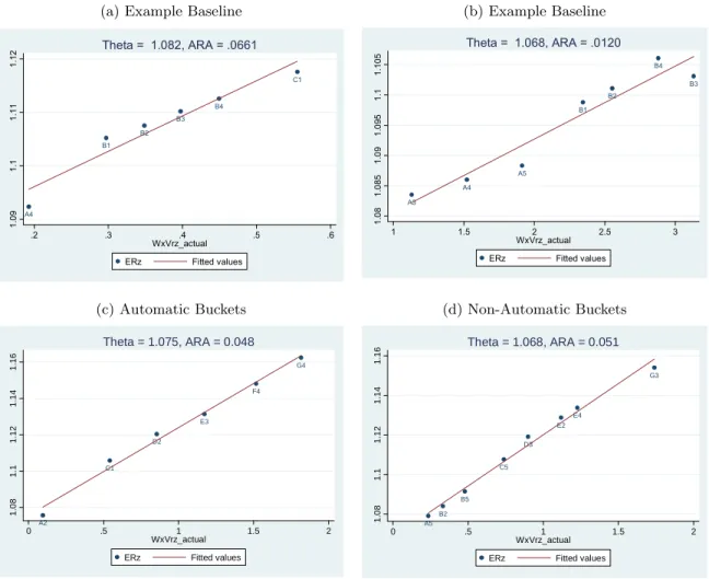
Panels (a) and (b) in Figure 2 show two examples of portfolio choices. The vertical axis measures the expected return of a risk bucket, E[Rz], and the horizontal axis measures the bucket variance
weighted by the investment amount, Wixi
zσz2/niz. The slope of the linear fit is our estimate of the
absolute risk aversion and it is reported on the top of each plot.
The error term captures deviations from the efficient portfolio due to measurement errors by investors, and real or perceived private information. The OLS estimates will be unbiased as long as the error component does not vary systematically with bucket risk. We discuss and provide evidence in support of this identification assumption below.
5.1 Results
The descriptive statistics of the estimated parameters of equation (9) for each portfolio choice are presented in Table 3. The average estimated ARA across all portfolio choices is 0.037 (column 1). Investors exhibit substantial heterogeneity in risk aversion, and its distribution is left skewed: the median ARA is 0.044 and the standard deviation 0.0245. This standard deviation overestimates the standard deviation of the true ARA parameter across investments because it includes the estimation error that results from having a limited number of buckets per portfolio choice. Following Arellano and Bonhomme (2012), we can recover the variance of the true ARA by subtracting the expected estimation variance across all portfolio choices. The calculated standard deviation of the true ARA is 0.0226, indicating that the estimation variance is small relative to the variance of risk aversion
across investments.28 The range of the ARA estimates is consistent with the estimates recovered in the laboratory. Holt and Laury (2002), for example, obtain ARA estimates between 0.003 and 0.109, depending on the size of the bet.
The experimental literature often reports the income-based RRA, defined in equation (8). To compare our results with those of laboratory participants, we report the distribution of the implied income-based RRA in Table 3, column 4. The mean income-based RRA is 2.81 and its distribution is right-skewed (median 1.62). This parameter scales the measure of absolute risk aversion according to the lottery expected income; therefore, it mechanically increases with the size of the bet. Column 3 of Table 3 reports the distribution of expected income from LC. The mean expected income is $125.6, substantially higher than the bet in most laboratory experiments. Not surprisingly, although the computed ARA in experimental work is typically larger than our estimates, the income-based RRA parameter is smaller, ranging from 0.3 to 0.52 (see for example Chen and Plott, 1998, Goeree et al., 2002, Goeree et al., 2003, and Goeree and Holt, 2004). Our results are comparable to Holt and Laury (2002), who also estimate risk aversion for agents facing large bets and (implicitly) find income-based RRA similar to ours, 1.2. Finally, Choi et al. (2007) report risk premia with a mean of 0.9, which corresponds to an income-based RRA of 1.8 in our setting. That paper also finds right skewness in their measure of risk premia.
Our findings imply that the high levels of risk aversion exhibited by subjects in laboratory experiments extrapolate to actual small-stake investment choices. Rabin and Thaler (2001, 2002) emphasize that such levels of risk aversion with small stakes are difficult to reconcile, within the expected utility framework over total wealth, with the observable behavior of agents in environments with larger stakes. Our results are subject to that critique. The median RRA computed using with our estimates of ARA and investors’ net-worth is 8,858 (average is 26,317).29 This suggests that EU framework on overall wealth cannot describe agents behavior in our environment. We show in on-line appendix A that the ARA estimated here describes the curvature of the utility function in other preference frameworks that are consistent with observed risk behavior over small and
28
The variance of the true ARA is calculated as:
varhARAii=varhARA[ii−E b
σ2ARAi
where the first term is the variance of the OLS ARA point estimates across all investments, and the second term is the average of the variance of the OLS ARA estimates across all investments.
29The Net-Worth based RRA reported here is computed asRRA
i=ARA[i·N Wi, whereN Wiis the mean point
large stake gambles. In particular, on-line appendix A.1 describes the optimal portfolio choice in a behavioral model in which utility depends (in a non-separable way) on both overall wealth level, W, and the flow of income from specific components of the agent’s portfolio,y.30 In such alternate preference specifications, agents’ ARA varies with, both, the level of overall wealth and the income flow generated by the gamble. This implies that the estimated level of ARA may be larger for small-stake gambles (i.e.,∂ARA(y, W)/∂y <0 ). Nevertheless, the elasticity of ARA with respect to investor’s wealth (i.e., ∂ARA∂W(y,W)ARAW(y,W)), our focus in the next section, is consistent in small and large stake environments.
Column 2 in Table 3 shows the estimates of the parameter θ, defined in equation (6), which captures the systematic component of LC. In our framework, the systematic component is driven by the common covariance between all LC bucket returns and the market, βL, or any potential
risk of the lending platform common to all risk buckets. The average estimated θ is 1.086, which indicates that the average investor requires a systematic risk premium of 8.6%. The estimated θ presents very little variation in the cross section of investors (coefficient of variation 3%), when compared to the variation in the ARA estimates (coefficient of variation of 66% ).31 Note that our ARA estimates are not based on this systematic risk premium; instead, they are based on the marginal premium required to take an infinitesimally greater idiosyncratic risk.
Table 4 presents the average and standard deviation of the estimated parameters by month. The average ARA increases from 0.029 during the first three months, to 0.039 during the last three (column 1). This average time series variation is potentially due to heterogeneity across investors as well as within investor variation, since not all investors participate in LC every month. The analysis in the next section disentangles the two sources of variation.
The estimatedθs, shown in column 2, imply that the average systematic risk premium increases from 5.7% to 8.9% between the first and last three months of the sample period. Note that the LC web page provides no information on the systematic risk of LC investments. Thus, this change is solely driven by changes in investors’ beliefs about the potential systematic risk of the
30
This is in line with Barberis and Huang (2001) and Barberis et al. (2006), which propose a framework where agents exhibit loss aversion over changes in specific components of their overall portfolio, together with decreasing relative risk aversion over their entire wealth. In the expected utility framework, Cox and Sadiraj (2006) propose a utility function with two arguments (income and wealth) where risk aversion is defined over income, but it is sensitive to the overall wealth level.
31As with the ARA, the estimation variance is small relative to the variance across investments. The standard
lending platform; that is, correlation between the likelihood of default of LC loans and aggregate macroeconomic shocks (covariance between LC returns and market returns, βL), or about the
expected market risk premium (E[Rm]), or about the functioning of the platform. This pattern
indicates that wealth shocks are potentially correlated with changes in investors’ beliefs about risk and return on financial assets. Thus, we cannot infer the elasticity of RRA to wealth by observing changes in the share of risky assets after a wealth shock, as they may be simply reflecting changes in beliefs about the underlying distribution of risky returns. Our proposed empirical strategy in the next section overcomes this identification problem.
5.2 Belief Heterogeneity and Bias: The Optimization Tool
Above we interpret the observed heterogeneity of investor portfolio choices as arising from differ-ences in risk preferdiffer-ences. Such heterogeneity may also arise if investors have different beliefs about the risk and returns of the LC risk buckets. Note that differences in beliefs about the systematic component of returns will not induce heterogeneity in our estimates of the ARA. This type of belief heterogeneity will be captured by variations inθ across investors.
The parameter θ will not capture heterogeneity of beliefs that affects the relative risk and expected return across buckets. This is the case if investors believe the market sensitivity of returns to be different across LC buckets, i.e. ifβi
z6=βLi for somez= 1, ...,35; or if investors’ priors
about the stochastic properties of the buckets idiosyncratic return differ from the ones computed in equations (1) and (2), i.e. Ei[R
z]6=E[Rz] orσzi 6=σz for somez= 1, ...,35. In such cases, the
equation characterizing the investor’s optimal portfolio is given by:
E[Rz] =θi+ ARAi·Bσi +Bµi +Biβ·W ixi z ni z σz2
This expression differs from our main specification equation (5) in three bias terms: Bσ ≡ σzi/σz
2 , Bµ≡ E[Rz]−Ei[Rz] / Wixizσz2/niz, and Bβ ≡ βzi −βLi /(Wixizσz2/niz).
Two features of the LC environment allow us to estimate the magnitude of the overall bias from these sources. First, LC posts on its website an estimate of the idiosyncratic default probabilities for each bucket. Second, LC offers an optimization tool to help investors diversify their loan portfolio. The tool constructs the set of efficient loan portfolios, given the investor’s total amount
in LC—i.e., the minimum idiosyncratic variance for each level of expected return. Investors then select, among all the efficient portfolios, the preferred one according to their own risk preferences. Importantly, the tool uses the same modeling assumptions regarding investors’ beliefs that we use in our framework: the idiosyncratic probabilities of default are the ones posted on the website and the systematic risk is common across buckets, i.e. βz =βL.32
Thus, we can measure the estimation bias by comparing, for the same investment, the ARA estimates obtained independently from two different components of the portfolio choice: the loans suggested by the tool and those chosen manually. If investors’ beliefs do not deviate systematically across buckets from the information posted on LC’s website and from the assumptions of the optimization tool, we should find investor preferences to be consistent across the two measures. Note that our identification assumption does not require that investors agree with LC assumptions. It suffices that the difference in beliefs does not vary systematically across buckets. For example, our estimates are unbiased if investors believe that the idiosyncratic risk is 20% higher than the one implied by the probabilities reported in LC, across all buckets. Note, moreover, that our test is based on investors’ beliefs at the time of making the portfolio choices. These beliefs need not to be correct ex post.
For this test we use the subsample of investments that combine buckets chosen through the optimization tool with buckets chosen manually. Then, for each investment, we independently compute the risk aversion implied by the component suggested by the optimization tool (Automatic buckets) and the risk aversion implied by the component chosen directly by the investor (Non-Automatic buckets). Panels (c) and (d) in Figure 2 provide an example of this estimation. Both panels plot the expected return and weighted idiosyncratic variance for the same portfolio choice. Panel (c) includes only the Automatic buckets, suggested by the optimization tool. Panel (d) includes only the Non Automatic buckets, chosen directly by the investor. The estimated ARA using the Automatic and Non-Automatic bucket subsamples are 0.048 and 0.051 respectively for this example.
We perform the independent estimation above for all portfolio choices that have at least two Automatic and two Non-Automatic buckets. To verify that investments that contain an Automatic component are representative of the entire sample, we compare the extreme cases where the entire
32
portfolio is suggested by the tool and those where the entire portfolio is chosen manually. The median ARA is 0.0455 and 0.0446 respectively, and the mean difference across the two groups is not statistically significant at the standard levels. This suggests that our focus in this subsection on investments with Automatic and Non-Automatic components is representative of the entire investment sample.
Table 5, panel A, reports the descriptive statistics of the ARA estimated using the Automatic and the Non-Automatic buckets. The average ARA is virtually identical across the two estimations (Table 5, columns 1 and 2). We calculate, for each investment, the difference between the two ARA estimates; Figure 3a shows the entire distribution of this difference and Column 3 of Table 5 reports its descriptive statistics. The mean is zero and the distribution of the difference is concentrated around zero, with kurtosis 11.53. This implies that the bias is close to zero not only in expectation, but investment-by-investment.
These results suggest that investors’ beliefs about the stochastic properties of the loans in LC do not differ substantially from those posted on the website. They also suggest that investors’ choices are consistent with the assumption that the systematic component is constant across buckets. Overall, these findings validate the interpretation that the observed heterogeneity across investor portfolio decisions is driven by differences in risk preferences.
In Table 5, panels B and C, we show that the difference in the distribution of the estimated ARA from the automatic and non-automatic buckets is insignificant both during the first and second halves of the sample period. This is key for interpreting the results in the next section, where we explore how the risk aversion estimates change in the time series with changes in house prices. Although we cannot directly rule out that changes in house prices are correlated with changes in beliefs for the same investor, we find that beliefs remain consistent with our assumptions in expectation throughout the sample period.
Table 5, columns 4 through 6, show that the estimated risk premia, θ, also exhibit almost identical mean and standard deviations when obtained independently using the Automatic and Non-Automatic investment components. Column 6 and Figure 3b show the distribution of the difference between the two estimates ofθfor thesame investment. They suggest that our estimates of the risk premium are unbiased.
risk of investing in LC do not change during the sample period. On the contrary, the observed average increase in the estimated systematic risk premium in Table 4 is also observed in panels B and C of Table 5: θ increases by 2.5 percentage points between the first and second halves of the sample. The results in Table 5 imply that changes in investors’ beliefs are fully accounted for by a common systematic component across all risk buckets and, thus, do not bias our risk aversion estimates.
6
Risk Aversion and Wealth
This section explores the relationship between investors’ risk taking behavior and wealth. We estimate the elasticity of ARA with respect to wealth, and use it to obtain the elasticity of RRA with respect to wealth, based on the following expression:
ξRRA,W =ξARA,W + 1, (10)
where ξRRA,W and ξARA,W refer to the wealth elasticities of RRA and ARA, respectively. For
robustness, we also estimate the elasticity of the income-based RRA in equation (8),ξρ,W.
We exploit the panel dimension of our data and estimate these elasticities, both, in the cross section of investors and, for a given investor, in the time series. In the cross section, wealthier investors exhibit lower ARA and higher RRA when choosing their portfolio of loans within LC; we refer to these elasticity estimates with the superscriptxs to emphasize that they do not represent the shape of individual preferences (i.e., ξxsARA,W, ξRRA,Wxs ,ξρ,Wxs ). And, in the time series, investor specific RRA increases after experiencing a negative wealth shock; that is, the preference function exhibits decreasing RRA. The contrasting signs of the cross sectional and investor-specific wealth elasticities indicate that preferences and wealth are not independently distributed across investors. Below, we describe our proxies for wealth in the cross section of investors, and for wealth shocks in the time series. Since the bulk of the analysis uses housing wealth as a proxy for investor wealth, we focus the discussion in this section on the subsample of investors that are home-owners.33
33None of the results in this section is statistically significant in the subsample of investors that are renters. This
is expected since housing wealth and total wealth are less likely to be correlated for renters, particularly in the time series. However, this is also possibly due to lack of power, since only a small fraction of the investors in our sample are renters.
6.1 Cross-Sectional Evidence
We use Acxiom’s imputed net worth as of October 2007 as a proxy for wealth in the cross section of investors. As discussed in Section 4, Acxiom’s imputed net worth is based on a proprietary algorithm that combines names, home address, credit rating, and other data from public sources. To account for potential measurement error in this proxy, we use a separate indicator for investor wealth in an errors-in-variable estimation: median house price in the investor’s zip code at the time of investment. Admittedly, house value is an imperfect indicator wealth; it does not account for heterogeneity in mortgage level or the proportion of wealth invested in housing. Nevertheless, as long as the measurement errors are uncorrelated across the two proxies, a plausible assumption in our setting, the errors-in-variable estimation provides an unbiased estimate of the cross-sectional elasticity of risk aversion to wealth.
We begin by exploring non-parametrically the relationship between the risk aversion estimates and our two wealth proxies for the cross section of home-owner investors in our sample. Figure 4 plots a kernel-weighted local polynomial smoothing of the risk aversion measure. The horizontal axis measures the (log) net worth and the (log) median house price in the investor’s zip code at the time of the portfolio choice. ARA is decreasing in both wealth proxies, while income-based RRA is increasing.
Turning to parametric evidence, we estimate the cross sectional elasticity of ARA to wealth using the following regression:
ln (ARAi) =β0+β1ln (N etW orthi) +ωi. (11)
The left hand side variable is investor i’s average (log) ARA, obtained by averaging the ARA estimates recovered from the investor’s portfolio choices during our sample period. The right-hand side variable is investor i’s imputed net worth. Thus, the estimated β1 corresponds to the
cross-sectional wealth elasticity of ARA,ξARA,Wxs .
To account for measurement error in our wealth proxy we estimate specification (11) in an errors-in-variables model by instrumenting imputed net worth with the average (log) house value in the zip code of residence of investor i during the sample period. Since the instrument varies only at the zip code level, in the estimation we allow the standard errors in specification (11) to be
clustered by zip code. The errors-in-variables approach works in our setting because risk preferences are obtained independently from wealth. If, for example, risk aversion were estimated from the share of risky and riskless assets in the investor portfolio, this estimate would inherit the errors in the wealth measure. As a result, any observed correlation between risk aversion and wealth could be spuriously driven by measurement errors. This is not a concern in our exercise.
Table 6 shows the estimated cross sectional elasticities with OLS and the errors-in-variables model. Our preferred estimates from the errors-in-variables model indicate that the elasticity of ARA to wealth in the cross section is -0.074 and statistically significant at the 1% confidence level (column 2). The non-parametric relationship is confirmed: wealthier investors exhibit a lower ARA. The OLS elasticity estimate is biased towards zero. This attenuation bias is consistent with classical measurement error in the wealth proxy.
The estimated ARA elasticity and equation (10) imply that the wealth-based RRA elasticity to wealth is positive, ξbxsRRA,W = 0.93. Columns 3 and 4 show the result of estimating specification
(11) using the income-based RRA as the dependent variable. The income-based RRA increases with investor wealth in the cross section, and the point estimate, 0.078, is also significant at the 1% level (column 4). The sign of the estimated elasticity coincides with that implied by the ARA elasticity. Overall, the results consistently indicate that the RRA is larger for wealthier investors in the cross section.
6.2 Within-Investor Estimates
The above elasticity, obtained from the variation of risk aversion and wealth in the cross section, can be taken to represent the form of the utility function of the representative investor only under strong assumptions. Namely, when the distributions of wealth and preferences in the population are independent.34 To identify the functional form of individual risk preferences we estimate the ARA elasticity using within-investor time series variation in wealth.
House values dropped sharply during our sample period.35 Since housing represents a substan-tial fraction of household wealth in the U.S., this decline implied an important negative wealth
34Chiappori and Paiella (2011) formally prove that any within-investor elasticity of risk aversion to wealth can be
supported in the cross section by appropriately picking such joint distribution.
35In this subsample the average zip code house price declines 4% between October 2007 and April 2008. In addition,
shock for home-owners.36 We use this source of variation, to estimate the wealth elasticity of investor-specific risk aversion in the subsample of home-owners that invest in LC:
ln (ARAit) =αi+β2ln (HouseV alueit) +t+ωit. (12)
The left-hand side variable is the estimated ARA for investor i in month t. The right-hand side variable of interest is the (log) median house value of the investor’s zip code during the month the risk aversion estimate was obtained (i.e., the month the investment in LC takes places). The right-hand side of specification (12) includes a full set of investor dummies as controls. These investor fixed effects (FE) account for all cross sectional differences in risk aversion levels. Thus, the elasticity β2 recovers the sensitivity of ARA to investor-specific shocks to wealth. We also
include a time-trend to absorb the evolution of housing prices, common to all investors, during the period under analysis.
By construction, the parameter β2 can be estimated only for the subsample of investors that
choose an LC portfolio more than once in our sample period. Although the average number of portfolio choices per investor is 2.0, the median investor chooses only once during our analysis period. This implies that the data over which we obtain the within investor estimates using (12) comes from approximately half of the original sample. To insure that the results below are rep-resentative for the full investor sample, we also show the results of estimating specification (12) without the investor FE to corroborate that the conclusions of the previous section are unchanged when estimated on the subsample of investors that chose portfolios more than once and controlling for time-trends.37
Table 7 reports the parameter estimates of specification (12), before and after including the investor FE. The FE results represent our estimated wealth elasticities of ARA, ξARA,W. The sign
of the estimated within-investor elasticity of ARA to wealth (column 2) is the same as in the cross section: absolute risk aversion is decreasing in investor wealth.
Equation (10) and the estimated wealth elasticity of ARA imply a negative wealth-based RRA
36
According to the Survey of Consumer Finances of 2007, the value of the primary residence accounts for approxi-mately 32% of total assets for the median U.S. family (see Bucks et al., 2009).
37
The estimates of ARA and the investment amount are statistically indistinguishable between those that invest once versus those that invest more than once (comparing only the first investment for those that invest more than once).
to wealth changes for a given investor, ξRRA,W, of -1.85. Column 4 report the result of estimating
specification (12) using the income-based RRA as the dependent variable. The point estimate, -4.35, also implies a negative relationship between this alternative measure of RRA and wealth. These results consistently suggest that investors’ utility function exhibits decreasing relative risk aversion.
The drop in house value is an incomplete measure of the change in the investor overall wealth. It is important, then, to analyze the potential estimation bias introduced by this measurement error. Classical measurement error would imply that the point estimate is biased towards zero; this estimate is therefore a lower bound (in absolute value) for the actual wealth elasticity of risk aversion. The (absolute value) of the elasticity could be overestimated if the percentage decline in house values underestimates the change in the investor’s total wealth. However, for error in measurement to account for the sign of the elasticity, the overall change in wealth has to be three times larger than the percentage drop in house value.38 This is unlikely in our setting since stock prices dropped 10% and investments in bonds had a positive yield during our sample period.39 Therefore, even if measurement error biases the numerical estimate, it is unlikely to affect our conclusions regarding the shape of the utility function. Finally, conditioning on investors that invest more than once in LC may introduce selection bias. If investors with large increments in risk aversion stop investing in LC, our computations would underestimate the effect of wealth shocks on risk aversion. If, on the other hand, investors with large negative wealth stop investing, our results would overestimate the wealth elasticity of risk aversion.
The observed positive relationship between investor RRA and wealth in the cross section from the previous section changes sign once one accounts for investor preference heterogeneity. The comparison of the estimates with and without investor FE in Table 7 confirms it. Moreover, we show in on-line appendix C.1 that the estimated elasticities of risk aversion to wealth, both in the cross-section of investors and for the same investor, are consistent with the observed relationship between the total investment amount in LC and wealth.40
38
We estimate the elasticity of ARA with respect to changes in house value to be –2.84. LetW be overall wealth
and H be house value, then: ξARA,W = ddlnlnARAW =−2.84·ddlnlnWH. The wealth elasticity of RRA is positive only if
ξARA,W >−1, which requires ddlnlnWH >2.84.
39Between October 1, 2007 and April 30, 2008 the S&P 500 Index dropped 10% and the performance of U.S.
investment grade bond market was positive —Barclays Capital U.S. Aggregate Index increased approximately 2%.
40
Since the ARA and elasticity estimates do not use information total investment in LC, this consistency test constitute an independent validation of our conclusions on investors’ risk taking behavior.
This implies that investors preferences and wealth are not independently distributed in the cross section. Investors with different wealth levels may have different preferences, for example, because more risk averse individuals made investment choices that made them wealthier. Alternatively, an unobserved investor characteristic, such as having more educated parents, may cause an investor the be wealthier and to be more risk averse. The results indicate that characterizing empirically the shape of the utility function requires, first, accounting for such heterogeneity.
7
Conclusion
In this paper we estimate risk preference parameters and their elasticity to wealth based on the actual financial decisions of a panel of U.S. investors participating in a person-to-person lending platform. The average absolute risk aversion in our sample is 0.037. We also measure the relative risk aversion based on the income generated by investing in LC (income-based RRA). We find a large degree of heterogeneity, with an average income-based RRA of 2.81 and a median of 1.61. These findings are similar to those obtained in experimental studies in the field and laboratories; they provide an external validation in a real life investment environment to the estimates obtained from experiments. We show that, since our estimates of risk aversion refer to the local curvature of preferences over changes in income, the parameters estimated here do not depend on a specific utility function and correctly describe agents’ preferences in different behavioral models.
We exploit the panel dimension of our data and estimate the elasticity of ARA and RRA with respect to wealth, both, in the cross section of investors and, for a given investor, in the time series. In the cross section, wealthier investors exhibit lower ARA and higher RRA when choosing their portfolio of loans within LC. For a given investor, the RRA increases after experiencing a negative wealth shock; that is, the average investor’s preference function exhibits decreasing RRA. The contrasting signs of the cross sectional and investor-specific wealth elasticities indicate that investors’ preferences and wealth are not independently distributed in the cross section. Therefore, to empirically characterize the shape of the utility function, one needs to take the properties of the joint distribution of preferences and wealth into account.