Zurich Open Repository and Archive University of Zurich Main Library Strickhofstrasse 39 CH-8057 Zurich www.zora.uzh.ch Year: 2017
Continuous Imputation of Missing Values in Streams of Pattern-Determining
Time Series
Wellenzohn, Kevin ; Böhlen, Michael H ; Dignös, Anton ; Gamper, Johann ; Mitterer, Hannes
Abstract: Time series data is ubiquitous but often incomplete, e.g., due to sensor failures and transmission errors. Since many applications require complete data, missing values must be imputed before fur- ther data processing is possible. We propose Top-k Case Matching (TKCM) to impute missing values in streams of time series data. TKCM defines for each time series a set of reference time series and exploits similar historical situations in the reference time series for the imputation. A situa- tion is characterized by the anchor point of a pattern that consists of l consecutive measurements over the reference time series. A missing value in a time series s is derived from the values of s at the anchor points of the k most similar patterns. We show that TKCM imputes missing values consistently if the reference time series pattern-determine time series s, i.e., the pattern of length l at time tn is repeated at least k times in the reference time se- ries and the corresponding values of s at the anchor time points are similar to each other. In contrast to previous work, we support time series that are not linearly correlated but, e.g., phase shifted. TKCM is resilient to consecutively missing values, and the accu- racy of the imputed values does not decrease if blocks of values are missing. The results of an exhaustive experimental evaluation using real-world and synthetic data shows that we outperform the state-of-the-art solutions.
DOI: https://doi.org/10.5441/002/edbt.2017.30
Posted at the Zurich Open Repository and Archive, University of Zurich ZORA URL: https://doi.org/10.5167/uzh-136704
Conference or Workshop Item
Originally published at:
Wellenzohn, Kevin; Böhlen, Michael H; Dignös, Anton; Gamper, Johann; Mitterer, Hannes (2017). Con-tinuous Imputation of Missing Values in Streams of Pattern-Determining Time Series. In: Proceedings of the 20th International Conference on Extending Database Technology, EDBT 2017, Venice, Italy, 21 March 2017 - 24 March 2017, 330-341.
Continuous Imputation of Missing Values
in Streams of Pattern-Determining Time Series
Kevin Wellenzohn Michael H. Böhlen
Department of Computer Science University of Zurich, Switzerland
{wellenzohn, boehlen}@ifi.uzh.ch
Anton Dignös Johann Gamper
Hannes Mitterer
Faculty of Computer Science Free University of Bolzano, Italy
[email protected]
ABSTRACT
Time series data is ubiquitous but often incomplete, e.g., due to sensor failures and transmission errors. Since many applications require complete data, missing values must be imputed before fur-ther data processing is possible.
We propose Top-kCase Matching (TKCM) to impute missing values in streams of time series data. TKCM defines for each time series a set of reference time series and exploits similar historical situations in the reference time series for the imputation. A situa-tion is characterized by theanchor pointof a pattern that consists of lconsecutive measurements over the reference time series. A missing value in a time seriessis derived from the values ofs
at the anchor points of thekmost similar patterns. We show that TKCM imputes missing valuesconsistentlyif the reference time seriespattern-determinetime seriess, i.e., the pattern of length
lat timetnis repeated at leastktimes in the reference time
se-ries and the corresponding values ofs at the anchor time points are similar to each other. In contrast to previous work, we support time series that are not linearly correlated but, e.g., phase shifted. TKCM is resilient to consecutively missing values, and the accu-racy of the imputed values does not decrease if blocks of values are missing. The results of an exhaustive experimental evaluation using real-world and synthetic data shows that we outperform the state-of-the-art solutions.
1.
INTRODUCTION
Time series data appears in many application domains, e.g., me-teorology, sensor networks, the financial world, and network mon-itoring. Often time series data is incomplete with values missing because of sensor failures, transmission errors, etc. Many applica-tions require complete data, hence missing values must be recov-ered before further data processing is possible.
Our research is motivated by the problem of missing values in the data collected by theSüdtiroler Beratungsring für Obst- und Weinbau(SBR). The SBR monitors and analyzes meteorological data streams in real time and alerts wine and apple farmers of po-tential harvest threats, such as frost, apple scab, and fire blight. The SBR operates a network of more than130weather stations in South
©2017, Copyright is with the authors. Published in Proc. 20th Inter-national Conference on Extending Database Technology (EDBT), March 21-24, 2017 - Venice, Italy: ISBN 978-3-89318-073-8, on OpenProceed-ings.org. Distribution of this paper is permitted under the terms of the Cre-ative Commons license CC-by-nc-nd 4.0
Tyrol, each of which records approximately20meteorological pa-rameters at a sample rate of five minutes. The measurements date back to 2007 with a total of 88.9M measurements. For illustration purposes, we use the temperature taken at one meter above ground level, which ranges from−20.3°C to+40.3°C and has a total of 7.8M (= 8%) missing values. Currently, missing values are manu-ally imputed by domain experts, based on the values at neighboring stations.
Various works have observed that time series are correlated and imputation techniques have been proposed that exploit the informa-tion of co-evolving time series [12, 13, 14, 16, 25]. Popular solu-tions include SVD based matrix decomposition techniques [11, 12], multivariate autoregression analysis [25], and PCA (principal com-ponent analysis) guided data summarization [16, 17, 23]. These approaches perform well if the time series are linearly correlated according to the Pearson correlation. The imputation accuracy de-teriorates if the time series are shifted and have a Pearson correla-tion close to zero.
In this paper, we propose Top-kCase Matching (TKCM) to im-pute missing values in streams of non-linearly correlated time se-ries. TKCM defines for each time seriessa small setRsof
ref-erence time series. If the value insat the current timetnis
miss-ing, TKCM defines aquery patternP(tn)that isanchoredattn
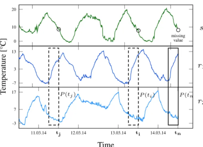
and composed of thelmost recent measurements of the reference time series. Then, thekmost similar non-overlapping patterns to the query pattern within a given time window are determined. The missing value is derived from the values of time seriessat the an-chor points of thekmost similar patterns. This process is illustrated in Fig. 1, where the value of the time seriessat the current timetn
is missing (small circle on the right). There are two reference time series ofs, i.e.,Rs ={r1, r2}. The query patternP(tn)is
com-posed of the snippets of the reference time series in the black frame. Thek= 2most similar patterns to the query pattern are anchored attiandtjand are shown as dashed rectangles. The missing value
ofsis derived from the values ofsat the anchor pointstiandtj
(small circles).
TKCM exploits two common properties of time series. First, time series often exhibit (not necessarily regularly) repeating pat-terns, also referred to as seasonal patterns. Second, time series are (not necessarily linearly) correlated in the sense that, whenever a pattern in a set of reference time series repeats, time seriess ex-hibits similar values. If these two properties are satisfied we say that at timetnthe reference time seriesRspattern-determinetime
seriess, denoted byRs, tnpd−→s. In other words, whenever
simi-lar patterns occur inRs, the values of time seriessare similar to each other, too. In contrast to previous work, this property allows not only linearly correlated reference time series but permits phase shifts. For instance, in Fig. 1 the two (shifted) reference time
se-T emperature [°C] s r1 r2 0 10 20 missing value -7 3 13 11.03.14 tj 12.03.14 13.03.14 ti 14.03.14 tn -3 7 17 P(tn P(ti) P(tj) Time
Figure 1: Imputation of a missing value ofsat timetn.
riesRs={r1, r2}pattern-determinetime seriessat timetn. We
show that TKCM imputes missing values consistently if the time series are pattern determining.
The paper makes the following technical contributions: • We present and formalize Top-kCase Matching (TKCM) to
impute missing values in streams of pattern-determining time series, which covers non-linear relationships between time series.
• We show that TKCM computes correct results for shifted time series that are not linearly correlated. We use a pattern of lengthl >1to exploit several consecutive measurements to find similar historical situations.
• We propose a dynamic programming scheme to find thek
non-overlapping patterns that minimize the sum of dissimi-larities with respect to the query pattern.
• We empirically show on real-world and synthetic datasets that TKCM: (a) outperforms state-of-the-art solutions, (b) can impute values in time series with phase shifts, and (c) is resilient to large blocks of consecutively missing values. The paper is structured as follows. Section 2 discusses related works. After the preliminaries in Section 3 we describe our ap-proach in Section 4. Section 5 analyzes the properties of TKCM and works out the differences between linear and non-linear cor-relations. In Section 6 we provide an implementation of TKCM that uses a dynamic programming solution to find the k non-overlapping patterns that are most similar to the query pattern. We continue with the experimental evaluation in Section 7 before we conclude this paper and present future research directions in Sec-tion 8.
2.
RELATED WORK
The need to recover missing data arises in many applications, ranging from meteorology [18, 26], to social science [20], machine learning [2], motion capture systems [14] and DNA microarray analysis [24]. Imputing a missing value means to recover it with a good estimate that is derived from intrinsic relationships in the underlying dataset.
Simple imputation techniques includemeanandmode imputa-tion [2], which replace the missing value with the mean or mode of
the same attribute. Interpolation techniques, such as linear interpo-lation and spline interpointerpo-lation, estimate the missing value from im-mediately preceding and succeeding values of the same attribute. If the gap is long, i.e., if many consecutive values are missing, these interpolation techniques perform badly. For instance, if an entire period of a sine wave is missing, linear interpolation would replace the gap with a straight line. Regression methods [25] estimate the missing value of a time series (e.g., temperature in Zurich) based on the value of other time series (e.g., temperature in Bern and Basel). Paulhus et al. [18] observed that nearby weather stations have similar values and computed a missing value at one station as the average of the values of nearby stations. Yozgatligil et al. [26] give a recent survey of imputation methods for meteorological time series and cover approaches based on neural networks and multiple imputation [19].
The ARIMA model [4] is a popular time series forecasting model that is a generalization of the auto-regressive (AR) model. ARIMA assumes a linear dependency of unknown future values on known past values of the time series. Finding the proper values forp, d, q
in an ARIMA(p, d, q) model is tedious, complex and involves man-ual analysis, known as the Box-Jenkins methodology [4].
Batista et al. [2] study the problem of missing data in the context of machine learning algorithms and present thek-Nearest Neigh-bor Imputation (kNNI) method to recover these values. For a multi-attribute object (e.g., breast cancer test with multiple mea-surements) that has a missing value for one attributeA, the kNNI approach looks forkobjects with similar values for the other at-tributes according to a distance metric that is not specified. The missing value is derived from the values of attributeAin these ob-jects. Troyanskaya et al. [24] extend kNNI to weight thekmost similar items according to their similarity. Our approach, TKCM, uses the concept of nearest neighbors (k most similar patterns), but is designed for time series streams and uses a two-dimensional query pattern for which thekmost similar non-overlapping pat-terns according to the Euclidean distance are searched.
Khayati et al. [11] propose REBOM to recover blocks of miss-ing values in irregular time series with non-repeatmiss-ing trends. The algorithm builds a matrix which stores the incomplete time series and thenmost linearly correlated time series according to Pear-son correlation. Missing values are first initialized, e.g., using lin-ear interpolation. Then the matrix is iteratively decomposed using theSingular Value Decomposition(SVD) method, where the least significant singular values are truncated. Due to the quadratic run-time complexity, REBOM does not scale to long run-time series. Next, Khayati et al. [12] present a solution with linear space complexity based on theCentroid Decomposition(CD), which is an approxi-mation of SVD. Unlike our approach, SVD and CD assume a lin-ear correlation between an incomplete time series and its reference time series. If time series are not linearly correlated, the imputation accuracy deteriorates since these trends are captured by the trun-cated least significant singular values. Khayati et al. [13] show that CD imputes more accurately than SVD when some reference time series are shifted and hence lowly linearly-correlated, because CD prioritizes highly linearly-correlated reference time series. Never-theless, their experiments show that adding more lowly-correlated reference time series has a negative impact on CD’s accuracy.
Sorjamaa et al. [15, 22] propose an imputation method based on a Self-Organizing-Map (SOM), which is an unsupervised learning technique based on neural networks. A combination of SVD and SOM [22] uses SVD for the imputation after initializing missing values in the matrix by a SOM classifier, whereas [15] combines two SOM classifiers for the imputation. Both methods are only evaluated on linearly correlated time series.
DynaMMo [14] is used for mining, summarizing, and imput-ing time series extracted from human motion capture systems. It is based on Kalman filters, which, similar to SVD, assume a lin-ear correlation between time series to accurately estimate unknown values. Moreover, unlike our approach, DynaMMo allows only one reference time series, which often is insufficient for an accurate im-putation.
The works most similar to our approach are MUSCLES [25] and SPIRIT [16, 17, 23], which focus on the online imputation of miss-ing values in streams of time series data. Both algorithms use vari-ants of auto-regressive (AR) models and exploit linear correlations between data streams. When the linear correlation diminishes, as in the case of shifted time series, none of the two approaches performs well.
MUSCLES [25] is an online algorithm that is based on a mul-tivariateauto-regression model, whose parameters are incremen-tally updated using the Recursive Least Squares method. Besides past values of the incomplete time series, MUSCLES takes also the most recent values of co-evolving and linearly correlated time se-ries into account that are within a windowp. How to choosepis not discussed; in the experimentsp = 6is used. Afterpconsecutive missing values, MUSCLES relies exclusively on imputed values for the incomplete time series. Since small imputation inaccuracies accumulate over a long stretch of missing values, MUSCLES ac-curacy deteriorates. Additionally, MUSCLES does not scale well to a large number of streams, unless an expensive offline subset selection on the time series is performed [17].
SPIRIT [16, 17, 23] uses an online Principal Component Analy-sis (PCA) to reduce a set ofnco-evolving and correlated streams to a small number ofkhidden variables that summarize the most important trends in the original data. For each hidden variable, SPIRIT fits one AR model on past values, which is incrementally updated as new data arrives. If a value is missing, the AR models are used to forecast the current value of each variable, from which an estimate of the missing value is derived. The imputed value, along with the non-missing values, is then used to update the fore-casting models. Updating the models with imputed models incurs similar problems as MUSCLES since inaccuracies are propagated. Since PCA and SVD are based on the same underlying principle, PCA shares SVD’s weaknesses for shifted time series.
From an implementation perspective, TKCM needs to find sim-ilar patterns in time series. This problem has been studied exten-sively for a single time series, yielding different dimensionality re-duction techniques, e.g., Discrete Fourier Transform [6], Piecewise Aggregate Approximation [7], and iSAX [21]. Keogh et al. [10] present a fast approach to find a subsequence (i.e., one-dimensional pattern), termed shapelet, of a time series that is most representa-tive for a set of time series. Finding patterns in our approach is more complex. We seek patterns that span several time series, and we have to select thekmost similar non-overlapping patterns. The main focus of this work is not performance, but an accurate impu-tation of shifted time series streams.
3.
PRELIMINARIES
Consider a setS={s1, s2, . . .}of streaming time series. Each
time series reports values from a sensor measured at time points
. . . , tn−2, tn−1, tn, wheretndenotes the current time, i.e., the time
of the latest measurement. The value of a time seriess ∈ Sat timetiis denoted ass(ti). We writes(tn) = NILto denote that the current value ofsis missing. W = {tn−L+1, . . . , tn−1, tn}
denotes theLtime points in our streaming window for which we keep measurements in main memory. We assume that the streaming windowW is long enough to include the query pattern andk
non-overlapping similar patterns.
For each time seriess ∈ Sthere exists an ordered sequence hr1, r2, . . .iof candidate reference time series, whereri∈S\ {s}.
They have been identified by domain experts and are consulted if the current value insis missing and must be recovered. The candi-date reference time series ofsare ranked according to how suitable they are for imputing a missing value ins. A single reference time series does not yield a robust method to estimate a missing value. Instead thedbest candidate reference time series that do not have a missing value at the current timetnare used. Lets ∈ Sbe an
incomplete time series withs(tn) = NIL. Thereference time
se-riesRsforsat the current timetnare the firstdtime series in the
ordered sequence for whichr(tn)6=NIL.
Note that there can be multiple incomplete time series with a missing value attn. For each incomplete time seriessi its
miss-ing valuesi(tn)is imputed individually using the respective set of
reference time seriesRs
i.
Example 1. As a running example, we use the four time se-ries in Table 2. The current time is tn = 14:20. Time
se-ries s is incomplete, hence the missing value at 14:20 must be imputed. We assume a sliding window of one hour, containing
L = 12measurements. For all time points beforetn the
val-ues either have been reported by the sensor or have been imputed, e.g.,r2(13:40) =18d.8°C. The candidate reference time series are
hr1, r2, r3i. At the current timetn =14:20, thed= 2reference
time series forsareRs ={r1, r2}. When the current time was tn=13:40, we hadRs ={r1, r3}sincer2(13:40)was missing.
✷
Notation Description
tn Current time
S={s1, s2, . . .} Set of time series
s(tn) =NIL Missing value of time seriessat timetn
ˆ
s(tn)6=NIL Imputed value of time seriessat timetn
d Number of reference time series
Rs={r1, . . . , rd} Set ofdreference time series fors
W ={. . . , tn} Time points in streaming window
L Length of streaming windowW
l Pattern length
P(ti) Pattern anchored at timeti
k Number of anchor points
A={ti1, . . . , tik} kmost similar anchor points
Table 1: Summary of notation.
4.
TOP-K CASE MATCHING (TKCM)
4.1
Approach
For the recovery of a missing value in an incomplete time series we look for patterns in the past when the values of the reference time series were similar to the current values.
Definition 1. (Pattern) LetRs={r1, . . . , rd}be the reference
time series for an incomplete time seriess. ThepatternP(ti)of
lengthl >0overRsthat is anchored at timetiis defined as ad×l
matrixP(ti)as follows:
P(ti) = ((r1(ti−l+1), . . . , r1(ti)),
..
. ...
Timet · · · 13:25 13:30 13:35 13:40 13:45 13:50 13:55 14:00 14:05 14:10 14:15 14:20
s · · · 22.8°C 21.4°C 21.8°C 23d.1°C 23.5°C 22.8°C 21.2°C 21.9°C 23.5°C 22.8°C 21.2°C NIL
r1 · · · 16.5°C 17.2°C 17.8°C 16.6°C 15.8°C 16.2°C 17.4°C 17.7°C 15.3°C 16.3°C 17.1°C 17.5°C
r2 · · · 20.3°C 19.8°C 18.6°C 18d.8°C 20d.0°C 20d.5°C 19.8°C 18.2°C 20.1°C 20.2°C 19.9°C 18.2°C
r3 · · · 14.0°C 14.8°C 13.6°C 13.0°C 14.5°C 14.3°C 14.0°C 15.0°C 13.0°C 14.5°C 14.3°C 14.6°C
Table 2: Time seriesswith a missing value at timetn=14:20 and the three reference time seriesr1, r2andr3.
A pattern is anchored at a time pointtiand consists of the values
fromti−l+1totiof each reference time series. Each row
repre-sents a subsequence of a reference time series, and each column represents the values of the reference time series at a time point. The pattern contains for each reference time series only the values at timeti, ifl= 1. The pattern includes additionally the preceding
l−1values, and hence captures the trend, ifl >1.
Example 2. Figure 2 shows two patterns over the reference time seriesRs ={r1, r2}in our running example (cf. Table 2). Both patterns have lengthl= 3and are anchored at time points 14:00 and 14:20, respectively. PatternP(14:00)contains one imputed value, namelyr2(13:50) = 20d.5°C. Sincel >1the pattern
cap-tures the current trend of the time series. ✷
16.2 17.4 17.7 [ 20.5 19.8 18.2 13:50 13:55 14:00 r1 r2 l= 3 d= 2 (a)P(14:00) 16.3 17.1 17.5 20.2 19.9 18.2 14:10 14:15 14:20 r1 r2 l= 3 d= 2 (b)P(14:20)
Figure 2: Two patterns of lengthl= 3overd= 2reference time series.
The pattern that is anchored at the current time is termedquery patternP(tn). We search in the reference time series for thek
patterns that are most similar toP(tn)using theL2norm.
Definition 2. (Pattern Dissimilarity) Let s be an incomplete time series with reference time seriesRsat timetn. The
dissimi-larity,δ, between two patternsP(tm)andP(tn)is defined as
δ(P(tm), P(tn)) = s X ri∈Rs X 0≤j<l (ri(tm−j)−ri(tn−j))2.
Example 3. The dissimilarity between the two patterns in Figure 2 is computed as follows: δ(P(14:00), P(14:20)) =
p
(17.7−17.5)2+ (17.4−17.1)2+ (16.2−16.3)2+. . . =
0.43. ✷
The dissimilarity measure is used to determine thekmost similar patterns to query patternP(tn). The anchor time points of thesek
patterns are referred to as thekmost similar anchor pointsA. Definition 3. (kMost Similar Anchor Points) LetP(tn)be the
query pattern for incomplete time seriessat timetnwith reference
time seriesRs, andLbe the length of the streaming time window. Thek most similaranchor pointstotn are a setA ⊆ W, with |A|=k, for which the following holds:
∀t∈A:tn−L+l≤t≤tn−l (1) ∀t, t′∈A:t6=t′→ |t−t′| ≥l (2) ∀A′: (1)∧(2)∧ |A′|=k→ X ti∈A δ(P(ti), P(tn))≤ X ti∈A′ δ(P(ti), P(tn)) (3)
The first condition states that all patterns are within the time win-dow and do not overlapP(tn). The second condition states that the
patterns do not overlap each other. The third condition ensures that the patterns that are anchored at the time points inAminimize the sum of the dissimilarities with respect to query patternP(tn).
We pick onlynon-overlappingpatterns to avoid near duplicates [5, 8]. Our experiments have shown that if overlapping patterns were allowed, thek most similar anchor points for some pattern
P(ti)are frequently time pointsti+1andti−1, which anchor the
first and second most similar patterns, etc. This is clearly not de-sired. Instead, non-overlapping patterns guarantee that we find a diverse set of patterns on which the imputation is based.
The missing value in the incomplete time seriessis the average of the values ofsat the most similar time points.
Definition 4. (Imputed Value) Letsbe a time series with refer-ence time seriesRsattnand missing values(tn). Furthermore,
letAbe thekmost similar time points to the current time. The imputed valuesˆ(tn)for time seriessat timetnis
ˆ s(tn) = 1 k X t∈A s(t). (4)
Example 4. Figure 3 shows a graphical representation of our running example (cf. Table 2). The value ofsat timetn =14:20
is missing and must be imputed. The query patternP(14:20)is framed in black. The two patterns most similar to the query pat-tern are shown as dashed rectangles and are anchored at time 14:00 and 13:35, respectively. Thus,A={14:00,13:35}are the anchor points. The missing value is computed as the average of the val-uess(14:00)ands(13:35):sˆ(14:20) = (21.9°C+ 21.8°C)/2 = 21.85°C. ✷ T emperature [°C] 21 23 15 17 13:25 13:3013:3513:40 13:45 13:50 13:5514:0014:05 14:10 14:15 tn= 14:20 18 20 Time s r1 r2
Figure 3: Thek = 2most similar non-overlapping patterns for query patternP(14:20)areP(14:00)andP(13:35).
5.
ANALYSIS
5.1
Correlation
A salient property of TKCM is its ability to handle time series that are shifted and hence not linearly correlated. The Pearson cor-relation, the most common correlation measure, quantifies the de-gree of linear correlation between time seriessandr, as
ρ(s, r) = P t∈W(s(t)−s¯)(r(t)−¯r) qP t∈W(s(t)−¯s)2 qP t∈W(r(t)−r¯)2 ,
wheres¯andr¯are the means of, respectively,sandrin windowW. Pearson correlation ranges from−1to1, indicating total negative and positive correlation, respectively. Thus,sandr are linearly correlated if|ρ(s, r)|is high. Ifρ(s, r) = 0time seriessandrare not linearly correlated.
Intuitively, a linear correlation ensures that (a) if one time series has close values for two time points, also the other has close values for these two time points and (b) if one time series has far apart values for two time points, also the other has far apart values for these two time points.
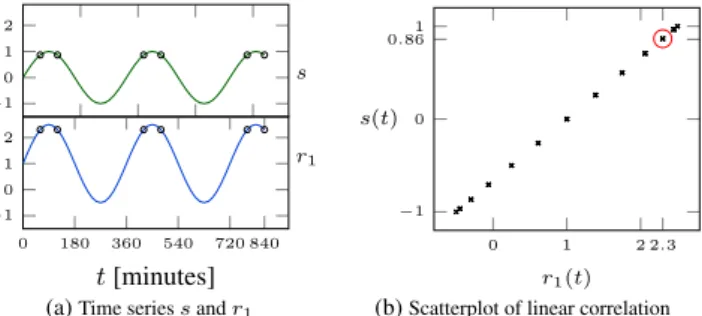
Example 5. Consider Figure 4a with time seriess(t) = sind(t)
andr1(t) = 1.5×sind(t) + 1, having different amplitudes and
offsets. The value ofr1att= 840isr1(840) = 2.3, and the same
valuer1(t)appears for time pointst∈ {780,480,420,120,60}.
Figure 4a illustrates that these are exactly the time points for which
shas the same value of s(840) = 0.86. Thus, the time series are perfectly linearly correlated. Figure 4b uses a scatterplot to display the correlation betweensandr1. The scatterplot displays
for each time pointtthe point(r1(t), s(t)). For instance, at time t= 840we haver1(840) = 2.3ands(840) = 0.86and the point
(2.3,0.86)is displayed in the scatterplot. The more the scatter-plot resembles a line with a non-zero slope, the higher the linear
correlation and hence Pearson correlation. ✷
s r1 −1 0 1 2 0 180 360 540 720 840 −1 0 1 2 t[minutes] (a)Time seriessandr1
0 1 2 2.3 −1 0 0.861 r1(t) s(t)
(b)Scatterplot of linear correlation
Figure 4: Linearly correlated time series s(t) = sind(t) and
r1(t) = 1.5×sind(t) + 1.
Example 5 illustrates how the imputation for linearly correlated time series works. Ifs(tn)is missing, we know that whenever time
seriesr1 observes valuer1(tn)(e.g., 2.3), time seriessobserves
the same values(t)(e.g., 0.86). Hence we can use values(t)for anytwherer1(t) = 2.3to impute values(tn).
In contrast, if the Pearson correlation approaches zero, s can have very different values although the reference time series has the same value. This is illustrated in Example 6.
Example 6. Figure 5a depicts the time seriess(t) = sind(t)and
r2(t) = sind(t−90). The two time series have the same amplitude
and offset but they are phase shifted. Time seriesr2 has the value r2(840) = 0.5also for time points t ∈ {600,480,240,120}.
However,shas different values, i.e., values(t) = 0.86for time pointst ∈ {480,120}and values(t) = −0.86for time points
t={600,240}. The scatterplot in Figure 5b shows that the data points do not cluster around a line, which means that they are non-linearly correlated. Their Pearson correlation is−0.0085. Note that for the same value ofr2(t)we can have two different values
fors(t). For instance, forr2(t) = 0.5we have eithers(t) = 0.86
ors(t) =−0.86. ✷ s r2 −1 0 1 2 0 180 360 540 720 840 −1 0 1 2 t[minutes] (a)Time seriessandr2
−1 0 0.5 1 −1 −0.86 0 0.861 r2(t) s(t)
(b)Scatterplot of non-linear correlation
Figure 5: Non-linearly correlated time seriess(t) = sind(t)and
r2(t) = sind(t−90)
Example 6 illustrates the key problem with non-linear correla-tions: the values of one time series can no longer be used to reli-ably determine a missing value in another time series. In the exper-iments we will see that this leads to imputations with a high root mean square error.
5.2
Pattern Length
The previous section illustrated that shifted time series that are not linearly correlated are difficult to handle. Intuitively, for shifted time series it is not sufficient to consider a single point in time. In-stead it is necessary to consider a pattern that includes neighboring time points to correctly relate time series. This section illustrates that a pattern with a lengthl >1improves the imputation for non-linear correlations. We writePl(t)to denote a pattern of lengthl
anchored at timet.
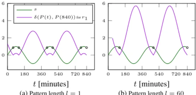
Example 7. Figure 6 displayssand, for each time pointt, the pattern dissimilarity of the pattern anchored atr1(t)to the query
patternP(840), i.e.,δ(P(t), P(840)). Figure 6a does this for pat-tern lengthl = 1. The pattern dissimilarity is zero whenever the value ofsis equal tos(840). Figure 6b shows what happens if we increase the pattern length tol= 60. Also for this case whenever the pattern dissimilarity for the reference time seriesr1is zero, i.e.,
for480and120, we have value0.86for time seriess. Observe that for increasing values oflless patterns with distance zero exist (e.g., two in Fig. 6b instead of 5 in Fig. 6a). But the patterns withl >1
at distance zero describe the situation better:s(840)is located at a down-slope, and in Fig. 6b values ofswhere the pattern distance is zero only exist at down-slopes, while in Fig. 6a we have such
values at both up- and down-slopes. ✷
Example 8. For shifted time series a pattern lengthl >1in ad-dition captures the trend of time series and yields a more accurate imputation. First, Figure 7a illustratessand the pattern dissimilar-ity tor2forl= 1. Figure 7b shows the same setting withl= 60.
With l > 1the pattern dissimilarity reaches zero only for time points480and120, where time seriesshas value0.86, which is the expected value for missing values(840). This illustrates that by increasingl, TKCM finds anchor points where the incomplete
0 180 360 540 720 840 0 2 4 6 t[minutes] s δ(P(t), P(840))forr1
(a)Pattern lengthl= 1
0 180 360 540 720 840 0 2 4 6 t[minutes] (b)Pattern lengthl= 60 Figure 6: A longer pattern reduces the number of patterns that are identical to the query pattern.
time seriesshas similar values and trends. Consequently, TKCM uses pattern lengthlto effectively deal with shifted time series that
are not linearly correlated. ✷
0 180 360 540 720 840 −1 0 1 2 3 t[minutes] s δ(P(t), P(840))forr2
(a)Pattern lengthl= 1
0 180 360 540 720 840 −1 0 1 2 3 t[minutes] (b)Pattern lengthl= 60 Figure 7: For shifted time series a longer pattern finds historical situations that are similar in value and trend.
LEMMA 5.1. (Monotonicity in Pattern Length) The number of patterns that are within a distanceτ to query patternP(tn)
de-creases as the pattern lengthlincreases:
|{tm|δ(Pl+1(tm), Pl+1(tn))≤τ}| ≤ |{tm|δ(Pl(tm), Pl(tn))≤τ}|
PROOF. Let ∆ = δ(Pl(tm), Pl(tn)). If pattern
length l is increased we get δ(Pl+1(tm), Pl+1(tn)) =
q
∆2+P
ri∈Rs(ri(tm−l)−ri(tn−l))
2. Observe that both
terms under the square root are non-negative, henceδ is mono-tonically increasing asl increases. It follows that the number of patterns with distance≤τdecreases aslgrows.
5.3
Consistent Imputation
Definition 5. (Pattern-Determining at timetn) At timetn the
reference time seriesRspattern-determinetime seriess, written
Rs, tnpd−→s, if for thekmost similar anchor pointsA(cf. Def. 3)
and patterns of lengthlthe following holds for a small valueǫ: ∀ti, tj∈A:|s(ti)−s(tj)| ≤ǫ
Example 9. In our running example (cf. Fig. 3), the query pattern P(tn=14:20) is based on the two reference time series
Rs = {r1, r2}. The k = 2 most similar anchor points are
A={14:00,13:35}, and the values ofsat these two anchors are 21.9°C and21.8°C, respectively. The two reference time series
Rspattern-determinesat timetn(writtenRs,14:20pd−→s) with
ǫ=|21.9°C−21.8°C|= 0.1°C. ✷
Pattern-determining time series guarantee that for a missing values(tn)we find in the sliding window at leastksimilar
pat-ternsP(ti1), . . . , P(tik)toP(tn)and the missing values(tn)is
similar to the observed valuess(ti).
Definition 6. (Consistent Time Series) Letsbe a time series with missing value s(tn) = NIL. Letsˆbe a time series where the missing values(tn)has been imputed, that issˆ(tn) 6= NILand ∀t ∈ W \ {tn} : ˆs(t) = s(t). Time seriessˆisconsistent if ∀t∈A:|sˆ(t)−sˆ(tn)| ≤ǫ.
When TKCM imputes an incomplete time seriess, we get an imputed time seriessˆ. Intuitively,sˆisconsistentif its value at the current timetnis similar to past values when the reference time
series observed a similar pattern.
LEMMA 5.2. Letsbe an incomplete time series with a missing values(tn) =NILandRsits reference time series. Letsˆbe the
imputed time series produced by TKCM. If (a)Rs, tnpd−→sand (b)
s(tn)is imputed as defined in Eq. 4,ˆsis a consistent time series.
PROOF. LetP(tn)be the query pattern that TKCM constructs
for the reference time series inRs with pattern lengthl. TKCM
looks for thekmost similar anchor pointsAwith respect toP(tn).
Since the reference time seriesRspattern-determinesat timetn,
we have that∀t, t′ ∈ A:|s(t)−s(t′)| ≤ǫ
. The imputed value
ˆ
s(tn)is the average ofsat the anchor points (cf. Eq. 4). Since all
values ofsatAare similar among each other within a distance of
ǫ, their meansˆ(tn)is equally similar within anǫdistance to all of
them, i.e.∀t∈A:|ˆs(t)−sˆ(tn)| ≤ǫ. Consequently the imputed
time seriessˆis consistent.
Next, we give an example of pattern-determining time series to illustrate what kind of phenomena TKCM can handle. Specifically, we show that sine waves of the formf(t) = A×sind(t360P +
φ) +owith amplitudeA, periodP, offseto, and phase shiftφare pattern-determining and that TKCM achieves consistent imputation on these series. The experiments in Section 7 confirm that this also holds for real world time series.
LEMMA 5.3. Assumes(t) =A1×sind(t360P +φ1) +o1and r(t) =A2×sind(t360P +φ2) +o2. ThenRs ={r}is
pattern-determiningsat timetnforl >1,k≥1andL≥kP+l.
PROOF. Observe that forl > 1, patternP(tn)occurs exactly
once every full period, i.e.,P(t) = P(tn)only ift=tn−iP for
everyi∈N. SinceL≥kP+lwe know there arekpatternsP(t), such thatP(t) =P(tn). Sinceshas the same periodicity asr, we
know that∀t, t′∈A:|s(t)−s(t′)| ≤0 =ǫ.
6.
IMPLEMENTATION OF TKCM
6.1
Overview
To impute a missing value in a time seriessat the current time
tn, TKCM performs three steps:
1. Pattern Extraction:Extract the anchor points of all candidate patterns from the streaming windowWand compute the dis-similarity of these patterns to query patternP(tn)(cf.
Defi-nition 2).
2. Pattern Selection:Select from the anchor points determined in step 1 the subsetAof the time points that anchor thek
3. Value Imputation: Impute the missing value attnusing
an-chor pointsA(cf. Definition 4).
In step 2, TKCM must find thekpatterns that neither overlap each other norP(tn), and that minimize the sum of dissimilarities
with respect toP(tn). A simple greedy algorithm that sorts the
an-chor points according to dissimilarity and picks the firstkones that do not overlap fails to minimize the sum of dissimilarities. There-fore, we propose a dynamic programming scheme that exploits an optimal sub-structure of this problem. LetD[j]denote the dissimi-larity between thejth pattern in the window and the query pattern, andM[i, j]denote the sum of dissimilarities of theimost simi-lar non-overlapping patterns from among the firstjpatterns inW, wherei≤ j. M[i, j] = 0ifi= 0, because no patterns have to be chosen. Similarly,M[i, j] =∞ifi > jbecause we cannot possibly findinon-overlapping patterns if we have onlyj < ito choose from. Otherwise, we have two options: either (a) we omit thejth pattern and pickipatterns that possibly overlap it; or (b) we pick thejth pattern having dissimilarityD[j]and have space left fori−1patterns that do not overlap it. In the latter case, the first pattern to no longer overlap thejth pattern, if one exists, is the
(j−l)th pattern.
This yields the following recurrence that minimizes the sum of dissimilarities: M[i, j] = 0 ifi= 0, ∞ ifi > j, min ( M[i, j−1] D[j] +M[i−1, j−l] otherwise (5)
The sum of dissimilarities of thekmost similar anchor points is given byM[k, L−2l+1], sinceL−2l+1is the number of anchor points when we exclude thel−1first andllast time points inW
(cf. Def. 3).
6.2
Algorithm
The implementation uses one ring buffer of lengthLfor each time seriessand an offset Ointo the ring buffers to efficiently update the streaming window. The value at timetn is located at
s[O]and the oldest value ats[(O+1)%L], where % is the modulo operator. TKCM’s pseudo code is listed in Algorithm 1. The input parameters are the ring buffer for the incomplete time seriesswith a missing value ats[O], dring buffers Rfor the reference time series, the window sizeL, the pattern lengthl, and the number of anchor pointsk. The algorithm stores the imputed value ins[O]
and returns it.
For processing, the algorithm uses an arrayD to store pattern dissimilarities, a(k+1)×(L−2l+2)matrixMto store the result for the dynamic programming algorithm, and an arrayAof sizek
to store thekmost similar anchor points.
Lines 1–7 correspond to step 1, where the dissimilarities of all patterns in W are computed and stored in array D. The first
l−1 and the last l time points are ignored as described above. In step 2, the algorithm finds the k most similar anchor points (Lines 8–23). Lines 8–14 implement the recurrence in Equation 5.
max(j−l,0) computes the predecessor of thejth pattern, yield-ingj= 0if no such predecessor exists. Once matrixMis filled,
M[k, L−2l+1] contains the sum of dissimilarities of thekmost similar anchor pointsA. Finally, TKCM backtracks in lines 15–23 to find the anchor pointsA. The algorithm starts in the lower-right most cellM[k, L−2l+1] and applies the recurrence back-wards. If for a cellM[i, j]we haveM[i, j] =M[i, j−1]thejth anchor point is skipped as it is not part of the optimal solution, and the algorithm proceeds at cellM[i, j−1]. Otherwise, thejth
Algorithm 1:TKCM
Input:Ring buffers, ArrayRofdring buffers, window sizeL,
pattern lengthl, andk.
Output:Imputed value ins[O].
1 forj←1toL−2∗l+1do 2 D[j]←0; 3 fori←0tod−1do 4 forx←0tol−1do 5 y←l+j−x−1; 6 D[j]←D[j]+(R[i][(O+y)%L]−R[i][(O−x)%L])2; 7 D[j]←sqrt(D[j]); 8 forj←0toL−2∗l+1do 9 M[0][j]←0; 10 fori←1tokdo 11 ifi > jthen 12 M[i][j]← ∞; 13 else 14 M[i][j]←min(M[i][j−1], D[j]+M[i−1][max(j−l,0)]); 15 i←k; 16 j←L−2∗l+1; 17 whilei >0do 18 ifM[i][j] =M[i][j−1]then 19 j−−; 20 else 21 A[i−1]←j; 22 i−−; 23 j←max(j−l,0); 24 s[O]←0; 25 fori←0tok−1do 26 s[O]←s[O] + (s[(O+l+A[i]−1)%L]/k); 27 returns[O];
anchor point is added toAand the algorithm proceeds with cell
M[i−1,max(j−l,0)]untilireaches 0, indicating thatkanchor points have been chosen. Finally, in lines 24–27, which correspond to step 3, the algorithm imputes the missing value using thekmost similar anchor points according to Definition 4.
Example 10. The top of Fig. 8 shows a streaming window of length L = 10 with current time tn = t13. The query
pat-tern of length l = 3and all extracted patterns are shown as red and black intervals, respectively. The first (i.e., j = 1) pattern isP(t6)and the last pattern isP(t10). The lower left table lists
the patterns in the streaming window, their indexj, predecessor, and dissimilarity with respect to query pattern P(t13). For
in-stance, P(t8) with indexj = 3has no non-overlapping
prede-cessor, hencemax(j−l,0) = 0. The right table shows the matrix
M computed by Algorithm 1. For instance,M[1,1]is the result of computingmin(D[1] +M[1−1,max(1−3,0)], M[1,1−1]) = min(0.5+0,∞) = 0.5. M[2,5] = 1.2in the lower-right corner contains the minimum sum of dissimilarity. To retrieve thekmost similar non-overlapping patterns, the algorithm starts atM[2,5]
and follows the highlighted path through the matrix: gray means that a pattern was omitted and green means that a pattern is part of the final result. For instance,M[2,5]is equal toM[2,4], hence the
j= 5th patternP(t10)is not part of the solution.M[2,4], in turn,
is the result ofD[4]+M[1,1] = 0.7+0.5 = 1.2, hencej = 4th patternP(t9)is part of the solution. Continuing withM[1,1]we
find another match before reachingM[0,0]. The algorithm finds thek= 2anchor pointsA={t6, t9}and computes the imputed valuesˆ(t13) =1/2(s(t6) +s(t9)).
t 4 5 6 7 8 9 10 11 12 13 P(6),δ=0.5 P(7),δ=0.3 P(8),δ=2.1 P(9),δ=0.7 P(10),δ=4.0 P(tn=t13 ) L=10 0 0 0 0 0 0 ∞ 0.5 0.3 0.3 0.3 0.3 ∞ ∞ ∞ ∞ 1.2 1.2 j= 0 1 2 3 4 5 i= 0 1 2 P(t) j max(j−l,0) D[j] P(t6 ) 1 0 0.5 P(t7 ) 2 0 0.3 P(t8 ) 3 0 2.1 P(t9 ) 4 1 0.7 P(t10 ) 5 2 4.0
Figure 8: Dynamic programming algorithm to compute the time points of the topk = 2non-overlapping patterns of lengthl= 3
that minimize the sum of dissimilarities.
6.3
Complexity Analysis
LEMMA 6.1. When the current timetnadvances, TKCM needs
O(1)time per streamsto update the corresponding ring buffer of sizeO(L).
PROOF. Whentnadvances, a new value replaces an old value
in the time series, requiringO(1)time in a ring buffer of sizeL.
LEMMA 6.2. The time complexity of TKCM to impute a missing value isO((l×d+k)×L).
PROOF. Initially TKCM computes the dissimilarity of O(L)
patterns, each of sizel×d, having an overall time complexity of
O(l×d×L). Next the algorithm iterates over theO(k×L)sized dynamic programming matrixM. Hence the overall time complex-ity isO(l×d×L+k×L).
LEMMA 6.3. The space complexity of TKCM to impute a miss-ing value isO(k×L).
PROOF. The pattern extraction phase requiresO(L) space to store the dissimilarities of all patterns. TKCM needsO(k×L)
space for matrixM.
7.
EXPERIMENTAL EVALUATION
In the experiments we simulate large blocks of consecutively missing values (e.g. one week). We repeatedly call TKCM to im-pute each missing value. This simulates a common sensor failure that requires a technician to reach a faulty weather station and re-place the broken sensor. As accuracy measure we use the root mean square error (RMSE), defined as
RMSE = s 1 |T| X tn∈T (s(tn)−sˆ(tn))2,
whereT is the set of missing time points. The experiments are conducted on a Linux server, running Ubuntu 14.04 server edition. It is powered by an Intel Xeon X5650 CPU with a frequency of 2.67GHz and 24GB of main memory. TKCM is implemented in C and compiled with Clang 3.4-1, based on LLVM 3.4.
7.1
Datasets and Setup
We use both real-world and synthetic datasets in our experimen-tal evaluation. First, we use the SBR dataset of meteorological time series in South Tyrol (cf. Sec. 1). Second, we shift the time series
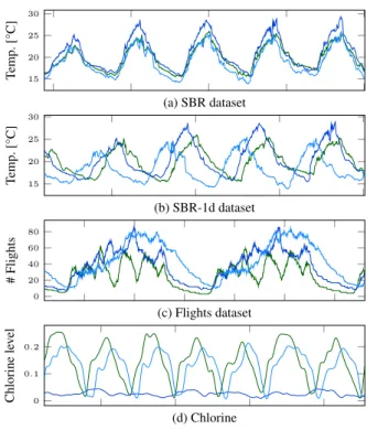
of the SBR data set by a (different) random amount up to one day and call this dataset SBR-1d. Third, we use the Flights dataset [3] that consists of eight time series, each of length 8801 (6 days). A time series describes at timetthe number of airplanes that departed from a given airport and are in the air at timet. Fourth, we use the publicly available Chlorine dataset [1] used by SPIRIT [16]. This synthetic dataset was generated by a simulation of a drinking water distribution system; it describes the chlorine concentration at 166 junctions over a time frame of 4310 time points (15 days) with a sample rate of 5 minutes. The propagation of the chlorine level in the system causes phase shifts in the dataset. Fig. 9 shows an excerpt of three sample time series from each dataset. Each time series has different amplitudes, phase shifts, and trends.
15 20 25 30 (a) SBR dataset T emp. [°C] 15 20 25 30 (b) SBR-1d dataset T emp. [°C] 0 20 40 60 80 (c) Flights dataset # Flights 0 0.1 0.2 (d) Chlorine Chlorine le v el
Figure 9: Three sample time series from each dataset. We compare TKCM to three competitors: CD [13] (provided by the author), MUSCLES [25] (implemented in Matlab), and SPIRIT [23] (obtained from [1], Matlab code). SPIRIT’s Matlab code does not impute missing values, hence we extended the code to use one autoregressive model per hidden variable as described in [23]. SPIRIT automatically adds or removes hidden variables as the streams evolve. When a hidden variable appears, a new autore-gressive model of orderp= 6needs to be fitted, which requires at leastpvalues of the new hidden variable before it can be used. If in that time a value needs to be imputed, the model is not yet ready. Consequently we fixed the number of hidden variables at two, which gave generally the best results in our experiments. For MUSCLES and SPIRIT we use a tracking window size ofp= 6as recommended by the authors [23, 25]. Contrary to the author’s rec-ommendation we set the exponential forgetting factorλto 1 rather than to0.96≤λ≤0.98. We found that forλ <1the accuracy de-creases, because the algorithms “forget” the old non-imputed (and accurate) values and adapt more to the new imputed (and inaccu-rate) values. CD has no parameters to tune. The code for our MUS-CLES, SPIRIT, and TKCM implementations is available online1.
1
7.2
Calibration
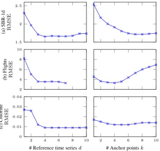
We begin with an initial calibration of TKCM’s parametersd,
k, andL. Unless otherwise noted we set the parameters to the following default values;d= 3reference time series,k= 5most similar anchor points, a streaming window ofL = 1year, and pattern lengthl= 72.
In the left column of Fig. 10 we show TKCM’s accuracy for increasing values ofdon three datasets; for brevity we omit the SBR dataset as it shows identical behavior to the SBR-1d dataset. TKCM’s accuracy significantly increases (that is theRMSE de-creases) asdincreases up tod = 3reference time series, while
d > 3does not provide significantly better accuracy. Since the Flights dataset has only8time series, we can setdat most to7. The right column of Fig. 10 shows the impact of parameterkon TKCM’s accuracy. In general we tend to pick small values ofk, e.g., k ∈ [3,10]to get the best possible (most similar) patterns from the window. Larger values ofkmay add less similar patterns, in particular for short streaming windows. We observed that for the two small datasets Flights and Chlorinek = 5is sufficient. TKCM’s accuracy noticeably decreases on the Flights dataset for
k >5, because the dataset contains only measurements for 6 days and if one day is missing we try to find more than5similar situa-tions within 5 days, which makes no sense. For the larger (1 year) SBR and SBR-1d datasets we found that there is a marginal accu-racy increase even fromk= 5tok= 10, after which the accuracy remains stable. Therefore, our recommendation is to use a small value ofk, e.g.k = 5, and if the dataset is large, one can safely doublek. 1.5 2 2.5 (a) SBR-1d R M S E 2 4 6 8 10 (b) Flights R M S E 2 4 6 8 10 0 0.01 0.02 0.03 0.04
# Reference time seriesd
(c) Chlorine R M S E 2 4 6 8 10 # Anchor pointsk
Figure 10: Calibration shows thatd = 3 andk = 5 are good default values.
For the small Flights and Chlorine datasets (6 and 15 days, re-spectively) we use in our experiments the entire time range as streaming window lengthL. For the SBR and SBR-1d datasets we use a streaming window lengthL = 105120 (1 year), be-cause one year covers the whole temperature range and contains each pattern several times. This choice is conservative; we found that already a window size of 6 months gives a good accuracy of
RMSE = 1.8°C, which only dropped to1.7°C for a 5 year
win-dow. In general, larger window sizesLprovide only a slightly superior accuracy.
7.3
Accuracy
7.3.1
Pattern Length
lFor shifted time series, the pattern lengthlis the key to an accu-rate and robust imputation. In Fig. 11, we evaluatelby varying the pattern lengthlfrom 1 to 144 (i.e., a pattern that spans 12 hours). As expected, for the (non-shifted) SBR datasetlhas close to no im-pact on TKCM’s accuracy, because there is a high linear correlation between the incomplete time series and itsd = 3reference time series. For the SBR-1d dataset theRMSEdrops by about 0.5°C (25%) by increasinglto 72. On the flight dataset we observe an improvement of 50% forl= 72and 60% forl= 144. The reason why we see an improvement beyondl= 72is the different sample rate of 1 minute of the Flights dataset as opposed to the 5 minutes in the SBR dataset. Whilel= 72yields a pattern that spans 6 hours in the SBR dataset, it only spans 1 hour in the Flights dataset. On the Chlorine dataset we observe an accuracy increase of 60% with pattern lengthl= 72, after which the accuracy slightly decreases.
1 36 72 108 144 0.6 0.8 1 1.2 1.4 (a) SBR:l R M S E 1 36 72 108 144 1.5 2 2.5 (b) SBR-1d:l R M S E 1 36 72 108 144 2 4 6 8 10 (c) Flights:l R M S E 1 36 72 108 144 0 0.01 0.02 0.03 0.04 (d) Chlorine:l R M S E
Figure 11: Pattern lengthlevaluated on each dataset. To put these raw numbers into perspective and see the real impact ofl, we compare TKCM’s recovery of an incomplete time seriess
in Fig. 12 with pattern lengthl = 1(left column) andl = 72
(right column). Observe how much TKCM’s recovery oscillates withl = 1and how well TKCM adapts to the assumed missing time seriesswithl= 72. Even for the SBR dataset there is a slight oscillation, albeit minimal compared to the three shifted datasets. The reason for this strong oscillation when l = 1is that with a short pattern, the reference time series do not pattern-determine the incomplete time series. The difference in dissimilarity between “good” patterns and “bad” patterns is too small for TKCM to de-tect, as explained in Sec. 5.1. Put differently, in the presence of shifts, time series are no longer linearly correlated; whenever a ref-erence time series observes a very similar value, the incomplete time series has very different values.
Fig. 13a shows the scatterplot of an incomplete time seriess
in the Chlorine dataset against one of its reference time series
r1. There is clearly no strong linear correlation (ρ(s, r1) =
0.5): e.g. forr1(t) = 0.1, s(t)has two different values (0and
0.15). Fig. 13b shows that the averageǫ(cf. Def. 5) decreases as lincreases on the Chlorine dataset with k = 5. Valueǫ = maxt,t′∈A|s(t)−s(t′)|essentially describes the range of the
val-ues ofsat thekmost similar anchor pointsA. The lowerǫgets, the
less the values ofsdiffer at the most similar anchor points, which indicates that the reference time series strongly pattern determines
15 20 25 (a) SBR T emp. [°C] s simputed by TKCM 15 20 25 (b) SBR-1d T emp. [°C] 20 40 60 (c) Fligths # Flights 0 0.1 0.2 l= 1 (d) Chlorine Chlorine le v el l= 72
Figure 12: The reason for the strong oscillation in TKCM’s recov-ery withl= 1are shifts in the reference time series. Increasing the pattern lengthlhelps TKCM to detect shifts.
coincides with our observations in Fig. 11d.
0 0.1 0.2 0 0.1 0.2 (a)r1(t) s ( t ) 1 36 72 108 144 0.04 0.05 0.06 (b) Pattern lengthl A v erage ǫ
Figure 13:Left: Scatterplot ofsagainst the reference time series
r1.Right:Range ofsat thekanchor points (Chlorine dataset).
7.3.2
Missing Block Length
In Fig. 14 we study TKCM’s accuracy in terms of the length of the missing block, i.e., the number of consecutively missing values that TKCM needs to impute. First, we use our large dataset SBR-1d and simulate sensor failures of up to several weeks. Fig. 14a shows that the accuracy of TKCM only slightly decreases by0.2°C as the block length grows from 1 to 4 weeks, after which the accuracy plateaus. Next, we increase the missing block length for the small dataset Chlorine from 10% to 80% of the dataset size. We start with the remaining 90% to 20% of the dataset in the streaming window of lengthL= 4310and impute the rest of the dataset as missing values. Fig. 14b shows that also for this case the accuracy decreases only slowly.
7.3.3
Comparison with Competitors
SBR.
We first perform a baseline comparison of all algorithms on the SBR dataset that has no phase shifts. Fig. 15a shows an excerpt2 4 6
1.5 2 2.5
(a) Block length [weeks]
R M S E 20 40 60 80 0 0.01 0.02 0.03 0.04 (b) Block length [% ofL] R M S E
Figure 14: Impact of the missing block length on the accuracy (Chlorine dataset).
of the experiment where we assume a block of values is missing in time seriess, and impute the missing values with each approach. TKCM, SPIRIT, MUSCLES, and CD perform virtually equally well. Observe that the last valley in the temperature curve shows a higher temperature than the previous valleys. While TKCM and CD are able to capture this trend, MUSCLES and SPIRIT impute a too low value. The most likely reason is that the models that MUS-CLES and SPIRIT build are not able to adapt quickly enough to the new behavior of the time series, while TKCM adapts instanta-neously to the changing behavior.
SBR-1d.
Next we impute the same block of missing values in the SBR-1d dataset that has shifted time series. Observe how TKCM’s accuracy only slightly decreases in Fig. 15b; TKCM slightly misses the second last downwards slope, but the last valley is again accu-rately imputed. SPIRIT completely misses the amplitude; its re-covered peaks are too low and its valleys are too high in tempera-ture. Moreover, the overall trend of the missing block is not well recovered. MUSCLES recovery is borderline at best; the overall periodicity of the signal is recovered, but MUSCLES was not able to recover any feature ofs. Moreover, shas a slightly increas-ing temperature trend, but MUSCLES’ recovery has a decreasincreas-ing trend. CD’s recovery is shifted with respect tos, as also indicated by the discontinuous imputation at the very beginning of the miss-ing block.Flights.
On the Flights dataset we observe a similar behavior as in the previous experiment. Fig. 15c shows that TKCM cap-tures each peak and valley accurately, while SPIRIT’s accuracy de-creases over time. Initially, the trend ofsis vaguely captured, but after the highest peak, the trend of SPIRIT’s imputation isinverse (i.e., peaks and valleys are swapped) with respect to the true sig-nal. Again, MUSCLES produces an extremely smoothed signal, that does not resemble the true time series; peaks and valleys are not recovered. CD’s recovery is only partially shown as many re-covered values arenegative. Most likely, the large block of missing values (ca. 20% of the dataset) is the reason.Chlorine.
In the Chlorine dataset TKCM captures the trend ofsgenerally well, the valleys are almost perfectly recovered, while the peaks are slightly less accurate. SPIRIT’s recovery does not capture the amplitude ofs, and also the trend of the recovery does not match that ofs. MUSCLES completely misses the first peak, imputing it with a valley instead; also the general trend of MUS-CLES’ recovery does not resemble s. In this dataset we found MUSCLES and SPIRIT to perform with widely differing accura-cies, sometimes their imputations is good, sometimes worse than in this example. There is no clear pattern when either approach works or fails. CD’s recovered signal has a very small amplitude and also the trend does not capture that ofs.
15 20 25 (a) SBR dataset T emp. [°C] s SPIRIT MUSCLES CD TKCM 15 20 25 (b) SBR-1d dataset T emp. [°C] 0 20 40 60 (c) Flight dataset # Flights 0 0.1 0.2 (d) Chlorine dataset Chlorine le v el
Figure 15: Imputation of incomplete time seriess with different imputation techniques on four different datasets.
Summary.
Fig. 16 shows theRMSEfor all compared algorithms on each dataset. In this comparison we impute 4 time series per data set; with missing block lengths per time series of 1 week in the SBR and SBR-1d datasets, and 20% of the dataset size for Flights and Chlorine. All algorithms are given the same amount of data (Lmeasurements per time series). We useL= 6months for the SBR and SBR-1d datasets, because of CD’s prohibitively large runtime forL = 1 year (our default) and the defaultL for the remain-ing datasets. The experiments show that only for the non-shifted SBR dataset all algorithms provide a comparable accuracy. For the remaining three shifted datasets, TKCM clearly outperforms its competitors both in terms of perceived accuracy (Fig. 15) and rawRMSE(Fig. 16). Our general observation is that non-shifted linearly-correlated data poses no significant challenge to any al-gorithm. As soon as shifts are present in the data, the accuracy of state-of-the-art solutions is largely unpredictable, ranging from good to unusable.
7.4
Runtime
As discussed in Sec. 6.3, TKCM’s time complexity is linear with respect to all parameters (l,d,k, andL) as confirmed by Fig. 17. In this experiments on the SBR-1d dataset we vary each parameter, leaving the other three parameters at their defaults (l= 72,d= 3,
k= 5andL= 1year). Fig. 17a and Fig. 17b show TKCM’s run-time with respect to the size of the query patternP(tn), Fig. 17c
shows the impact of the number of anchor pointsk, and Fig. 17d shows the impact of the streaming window sizeLon the runtime. ParameterLhas the largest impact on TKCM’s runtime, followed
0 2 4 6 1.07 0.88 0.89 1.32 SBR R M S E TKCM SPIRIT MUSCLES CD 0 2 4 6 1.82 2.57 4.34 2.12 SBR-1d R M S E 0 10 20 3.57 14.67 8.35 20.7 Flights R M S E 0 0.02 0.04 0.06 0.08 0.014 0.049 0.036 0.054 Chlorine R M S E
Figure 16: Comparison of TKCM, SPIRIT, MUSCLES, and CD for each dataset.
bylanddwith similar impact. Parameterkis relatively cheap – even if set to very large values, e.g.,k >50. For our default pa-rameter settings we observe a runtime of approximately 2 seconds to impute a single missing value.
50 100 0 2 4 6 8
(a) Pattern lengthl
Runtime
(sec)
1 2 3 4 5
(b) # reference time seriesd
100 200 300 0 2 4 6 8 (c) # anchor pointsk Runtime (sec) 1 2 3 4
(d) Window sizeL(years)
Figure 17: Runtime experiments. TKCM’s time complexity is linear with respect to all its parametersl, d, k, andL (SBR-1d dataset).
Performance breakdown.
As described in Sec. 6 the twomain phases of TKCM arepattern extraction(PE) andpattern se-lection(PS). In our default setup, the PE-phase accounts for 92% of TKCM’s overall runtime. If we further subdivide the PE-phase, we see that 82% of the overall runtime are required to fetch data from main memory and 10% are used to compute the pattern dissimilar-ityδ. If we increasekto300we see the runtime of the PS-phase climbing from 8% up to 25%. Thus, for the default value ofk, the runtime incurred by the PS-phase is outweighed by the PE-phase. Hence, to improve TKCM’s performance, future research must fo-cus on speeding up the pattern extraction phase.
Comparison.
A direct comparison of the runtimes of the con-sidered approaches is not meaningful, because the systems are im-plemented in different programming languages (TKCM in C, CD in Java, MUSCLES and SPIRIT in Matlab). To give a rough feeling for the overall performance we consider each approach in turn. CD is an offline algorithm and not applicable to streams. CD’s matrix decomposition lasted in our experiments roughly 20 minutes per execution and is hence not applicable to streaming environments. Both SPIRIT and MUSCLES required one millisecond to impute one missing value, TKCM requires roughly 2 seconds.8.
CONCLUSION AND FUTURE WORK
We studied the problem of missing values in meteorological streams of time series data and presented an algorithm, termed TKCM, to accurately impute missing values in a streaming envi-ronment. If the current value in a time seriessis missing, TKCM determines a two-dimensional query pattern over the lastl mea-surements ofdreference time series. It then retrieves the anchor points of thekmost similar non-overlapping patterns to the query pattern. The missing value is computed from the values ofs at thesekanchor points. We show that TKCM achieves consistent imputation if the reference time series pattern-determines, which covers non-linear relationships between time series such as phase shifts. An extensive experimental evaluation using four real-world and synthetic datasets confirms that TKCM is accurate and outper-forms state-of-the-art competitors.
Future work points in several directions. First, we will work on the efficiency of TKCM, in particular the pattern extraction phase, which proved to be the most time-consuming component. In partic-ular, we plan to reduce the number of extracted patterns by pruning patterns that cannot possibly belong to an optimal solution. Sec-ond, we plan to investigate how to automatically determine the best candidate reference time series, although in many application do-mains (and especially in meteorology) we can rely on human ex-perts. Third, we plan to compare different dissimilarity functionsδ
(e.g.L1-norm, DTW [9], etc.). Moreover, it would be interesting
to compute an alignment between shifted time series (e.g., using DTW [9]) and to compare TKCM’s accuracy on the aligned time series using a pattern lengthl = 1to the accuracy on the shifted time series usingl >1.
9.
ACKNOWLEDGMENTS
The work has been done as part of the DASA project, which is funded by the Foundation of the Free University of Bozen-Bolzano. We wish to thank our partners at the Südtiroler Beratungsring and the Research Centre for Agriculture and Forestry Laimburg for the good collaboration and helpful domain insights they provided, in particular Armin Hofer, Martin Thalheimer, and Robert Wiedmer. We also want to thank Mourad Khayati for his input and for sharing his CD implementation used in the experimental evaluation. We thank the anonymous reviewers for their valuable comments and suggestions.
10.
REFERENCES
[1] SPIRIT project.
https://www.cs.cmu.edu/afs/cs/project/spirit-1/www/. Accessed: 2016-05-29.
[2] G. E. A. P. A. Batista and M. C. Monard. An analysis of four missing data treatment methods for supervised learning. Applied Artificial Intelligence, 17(5-6), 2003.
[3] A. Behrend and G. Schüller. A case study in optimizing continuous queries using the magic update technique. In SSDBM, pages 31:1–31:4, 2014.
[4] G. E. P. Box and G. Jenkins.Time Series Analysis, Forecasting and Control. Holden-Day, Incorporated, 1990. [5] B. Chiu, E. Keogh, and S. Lonardi. Probabilistic discovery of
time series motifs. InKDD, pages 493–498, 2003. [6] C. Faloutsos, M. Ranganathan, and Y. Manolopoulos. Fast
subsequence matching in time-series databases.SIGMOD Rec., 23(2):419–429, May 1994.
[7] E. Keogh, K. Chakrabarti, M. Pazzani, and S. Mehrotra. Dimensionality reduction for fast similarity search in large
time series databases.Knowledge and information Systems, 3(3):263–286, 2001.
[8] E. Keogh, J. Lin, and A. Fu. HOT SAX: Efficiently finding the most unusual time series subsequence. InICDM, pages 226–233, 2005.
[9] E. J. Keogh. Exact indexing of dynamic time warping. In VLDB, 2002.
[10] E. J. Keogh and T. Rakthanmanon. Fast shapelets: A scalable algorithm for discovering time series shapelets. InICDM, pages 668–676, 2013.
[11] M. Khayati and M. H. Böhlen. REBOM: recovery of blocks of missing values in time series. InCOMAD, pages 44–55, 2012.
[12] M. Khayati, M. H. Böhlen, and J. Gamper. Memory-efficient centroid decomposition for long time series. InICDE, pages 100–111, 2014.
[13] M. Khayati, P. Cudré-Mauroux, and M. H. Böhlen. Using lowly correlated time series to recover missing values in time series: a comparison between SVD and CD. InSSTD, pages 237–254, 2015.
[14] L. Li, J. McCann, N. S. Pollard, and C. Faloutsos. DynaMMo: Mining and summarization of coevolving sequences with missing values. InKDD, pages 507–516, 2009.
[15] P. Merlin, A. Sorjamaa, B. Maillet, and A. Lendasse. X-SOM and L-SOM: A double classification approach for missing value imputation.Neurocomputing, 73(7-9):1103–1108, 2010.
[16] S. Papadimitriou, J. Sun, and C. Faloutsos. Streaming pattern discovery in multiple time-series. InVLDB, pages 697–708, 2005.
[17] S. Papadimitriou, J. Sun, C. Faloutsos, and P. S. Yu. Dimensionality reduction and filtering on time series sensor streams. InManaging and Mining Sensor Data, pages 103–141. 2013.
[18] J. L. H. Paulhus and M. A. Kohler. Interpolation of Missing Precipitation Records.Monthly Weather Review, 80(8), Aug. 1952.
[19] D. Rubin. Multiple Imputation after 18+ Years.Journal of the American Statistical Association, 91(434), 1996. [20] J. L. Schafer and J. W. Graham. Missing data: our view of
the state of the art.Psychological Methods, 7, 2002. [21] J. Shieh and E. Keogh. iSAX: Indexing and mining terabyte
sized time series. InKDD, pages 623–631, 2008. [22] A. Sorjamaa, P. Merlin, B. Maillet, and A. Lendasse.
SOM+EOF for finding missing values. InESANN, pages 115–120, 2007.
[23] J. Sun, S. Papadimitriou, and C. Faloutsos. Online latent variable detection in sensor networks. InICDE, pages 1126–1127, 2005.
[24] O. G. Troyanskaya, M. N. Cantor, G. Sherlock, P. O. Brown, T. Hastie, R. Tibshirani, D. Botstein, and R. B. Altman. Missing value estimation methods for DNA microarrays. Bioinformatics, 17(6), 2001.
[25] B. Yi, N. Sidiropoulos, T. Johnson, H. V. Jagadish, C. Faloutsos, and A. Biliris. Online data mining for co-evolving time sequences. InICDE, pages 13–22, 2000. [26] C. Yozgatligil, S. Aslan, C. Iyigun, and I. Batmaz.
Comparison of missing value imputation methods in time series: the case of turkish meteorological data.Theoretical and Applied Climatology, 112(1-2), 2013.