Mean Field Multi-Agent Reinforcement Learning

Mean Field Multi-Agent Reinforcement Learning

Abstract

Existing multi-agent reinforcement learning meth-ods are limited typically to a small number of agents. When the agent number increases largely, the learning becomes intractable due to the curse of the dimensionality and the exponential growth of agent interactions. In this paper, we present Mean Field Reinforcement Learningwhere the interactions within the population of agents are approximated by those between a single agent and the average effect from the overall population or neighboring agents; the interplay between the two entities is mutually reinforced: the learning of the individual agent’s optimal policy depends on the dynamics of the population, while the dy-namics of the population change according to the collective patterns of the individual policies. We develop practical mean field Q-learning and mean field Actor-Critic algorithms and analyze the con-vergence of the solution to Nash equilibrium. Ex-periments on Gaussian squeeze, Ising model, and battle games justify the learning effectiveness of our mean field approaches. In addition, we re-port the first result to solve the Ising model via model-free reinforcement learning methods.

1. Introduction

Multi-agent reinforcement learning (MARL) is concerned with a set of autonomous agents that share a common en-vironment (Busoniu et al., 2008). Learning in MARL is fundamentally difficult since agents not only interact with the environment but also with each other. IndependentQ -learning (Tan, 1993) that considers other agents as a part of the environment often fails as the multi-agent setting breaks the theoretical convergence guarantee and makes the learn-ing unstable: changes in the policy of one agent will affect that of the others, and vice versa (Matignon et al., 2012).

1_{University College London, London, United Kingdom.} 2_{Shanghai Jiao Tong University, Shanghai, China.}∗_Equal Con-tribution. Correspondence to: Jun Wang <[email protected]>, Yaodong Yang <[email protected]>.

Proceedings of the35t h _{International Conference on Machine}

Learning, Stockholm, Sweden, PMLR 80, 2018. Copyright 2018 by the author(s).

Instead, accounting for the extra information from conjec-turingthe policies of other agents is beneficial to each single learner (Foerster et al., 2017; Lowe et al., 2017a). Studies show that an agent who learns the effect of joint actions has better performance than those who do not in many scenarios, including cooperative games (Panait & Luke, 2005), zero-sum stochastic games (Littman, 1994), and general-zero-sum stochastic games (Littman, 2001; Hu & Wellman, 2003). The existing equilibrium-solving approaches, although prin-cipled, are only capable of solving a handful of agents (Hu & Wellman, 2003; Bowling & Veloso, 2002). The compu-tational complexity of directly solving (Nash) equilibrium would prevent them from applying to the situations with a large group or even a population of agents. Yet, in practice, many cases do require strategic interactions among a large number of agents, such as the gaming bots in Massively Multiplayer Online Role-Playing Game (Jeong et al., 2015), the trading agents in stock markets (Troy, 1997), or the online advertising bidding agents (Wang et al., 2017). In this paper, we tackle MARL when a large number of agents co-exist. We consider a setting where each agent is directly interacting with a finite set of other agents; through a chain of direct interactions, any pair of agents is intercon-nected globally (Blume, 1993). The scalability is solved by employing Mean Field Theory (Stanley, 1971) – the interac-tions within the population of agents are approximated by that of a single agent played with the average effect from the overall (local) population. The learning is mutually rein-forced between two entities rather than many entities: the learning of the individual agent’s optimal policy is based on the dynamics of the agent population, meanwhile, the dynamics of the population is updated according to the in-dividual policies. Based on such formulation, we develop practical mean fieldQ-learning and mean field Actor-Critic algorithms, and discuss the convergence of our solution under certain assumptions. Our experiment on a simple multi-agent resource allocation shows that our mean field MARL is capable of learning over many-agent interactions when others fail. We also demonstrate that with temporal-difference learning, mean field MARL manages to learn and solve the Ising model without even explicitly knowing the energy function. At last, in a mixed cooperative-competitive battle game, we show that the mean field MARL achieves high winning rates against other baselines previously re-ported for many agent systems.

2. Preliminary

MARL intersects between reinforcement learning and game theory. The marriage of the two gives rise to the general framework ofstochastic game(Shapley, 1953).

2.1. Stochastic Game

AnN-agent (or,N-player) stochastic gameΓis formalized by the tupleΓ , S,A1, . . . ,AN,r1_{, . . . ,r}N_{,p, γ, where}

Sdenotes the state space, andAjis the action space of agent

j∈ {1, . . . ,N}. The reward function for agentjis defined asrj _:S×A1_{× · · · ×A}N_{→R, determining the immediate}

reward. The transition probabilityp:S_×A1_{×· · ·×}AN _→

Ω(S)characterizes the stochastic evolution of states in time, withΩ(S)being the collection of probability distributions

over the state spaceS. The constantγ_∈[0,1)represents the

reward discount factor across time. At time stept, all agents take actions simultaneously, each receives the immediate rewardrj

t as a consequence of taking the previous actions.

The agents choose actions according to their policies, also known as strategies. For agentj, the corresponding policy is defined asπj _:S→Ω(Aj_{), whereΩ(A}j_{)is the collection}

of probability distributions over agentj’s action spaceAj.

Letπ,[π1_{, . . . , π}N_{]denote the joint policy of all agents;}

we assume, as one usually does,πto be time-independent, which is referred to bestationary. Provided an initial state s, the value function of agentjunder the joint policyπis written as the expected cumulative discounted future reward:

vπ(j s) =vj(s;π) =

∞ X

t=0

γtEπ,prtj|s0=s,π. (1)

TheQ-function (or, the action-value function) can then be defined within the framework ofN-agent game based on the Bellman equation given the value function in Eq. (1) such that theQ-functionQj

π:S×A1× · · · ×AN→Rof agent

junder the joint policyπcan be formulated as Qj

π(s,a) =rj(s,a) +γEs0_∼p[vπj(s0)], (2)

wheres0_{is the state at the next time step. The value function}

vπj can be expressed in terms of theQ-function in Eq. (2) as

v_πj(s) =Ea∼πQπj(s,a)

. (3)

TheQ-function forN-agent game in Eq. (2) extends the formulation for single-agent game by considering the joint action taken by all agentsa,[a1_{, . . . ,a}N_{], and by taking}

the expectation over the joint action in Eq. (3).

We formulate MARL by the stochastic game with a discrete-time non-cooperative setting,i.e.no explicit coalitions are considered. The game is assumed to be incomplete but to have perfect information (Littman, 1994),i.e. each agent knows neither the game dynamics nor the reward functions of others, but it is able to observe and react to the previous actions and the resulting immediate rewards of other agents.

2.2. NashQ-learning

In MARL, the objective of each agent is to learn an optimal policy to maximize its value function. Optimizing thevπj

for agentjdepends on the joint policyπof all agents, the concept ofNash equilibriumin stochastic games is therefore of great importance (Hu & Wellman, 2003). It is represented by a particular joint policyπ_∗,[π1

∗, . . . , π∗N]such that for alls_∈S, j_{∈ {}1, . . . ,N_}and all validπj_{, it satisfies}

vj(s;π_∗) =vj(s;π_∗j,π−j

∗ )≥vj(s;πj,π∗−j). Here we adopt a compact notation for the joint policy of all agents exceptjasπ∗−j ,[π1∗, . . . , π

j−1

∗ , π∗j+1, . . . , π∗N]. In a Nash equilibrium, each agent acts with thebest response π_∗j to others, provided that all other agents follow the policy

π_∗−j. It has been shown that, for aN-agent stochastic game, there is at least one Nash equilibrium with stationary policies (Fink et al., 1964). Given a Nash policyπ_∗, the Nash value functionvNash_(s),[v1

π_∗(s), . . . ,vπN_∗(s)]is calculated with

all agents followingπ∗from the initial statesonward. NashQ-learning (Hu & Wellman, 2003) defines an iterative procedure with two alternating steps for computing the Nash policy: 1) solving the Nash equilibrium of the current stage game defined by{Qt}using the Lemke-Howson algorithm

(Lemke & Howson, 1964), 2) improving the estimation of theQ-function with the new Nash equilibrium value. It can be proved that under certain assumptions, the Nash operator

HNash_{defined by the following expression}

HNashQ(s,a) =Es0_∼pr(s,a) +γvNash(s0) (4)

forms a contraction mapping, whereQ , [Q1_{, . . . ,Q}N_],

andr(s,a),[r1_{(s,a), . . . ,r}N_{(s,a)]. TheQ-function will}

eventually converge to the value received in a Nash equilib-rium of the game, referred to as theNash Q-value.

3. Mean Field MARL

The dimension of joint actionagrows proportionallyw.r.t. the number of agentsN. As all agents act strategically and evaluate simultaneously their value functions based on the joint actions, it becomes infeasible to learn the standard Q-functionQj_{(s,a). To address this issue, we factorize the}

Q-function using only the pairwise local interactions: Qj_{(s,a) =} 1

Nj

X

k∈N(j)

Qj_(s,aj_,ak_{), (5)}

whereN(j)is the index set of the neighboring agents of agentjwith the sizeNj _{=|N(j)|determined by the settings}

of different applications. It is worth noting that the pairwise approximation of the agent and its neighbors, while signif-icantly reducing the complexity of the interactions among agents, still preserves global interactions between any pair of agents implicitly (Blume, 1993). Similar approaches can be found in factorization machine (Rendle, 2012) and learning to rank (Cao et al., 2007).

3.1. Mean Field Approximation

The pairwise interactionQj_(s,aj_,ak_{)as in Eq. (5) can be}

approximated using the mean field theory (Stanley, 1971). Here we consider discrete action spaces, where the action aj_{of agentjis a discrete categorical variable represented as}

the one-hot encoding with each component indicating one of theDpossible actions:aj_,[aj

1, . . . ,a j

D]. We calculate the

meanactiona¯j_{based on the neighborhoodN(j)of agent}

j, and express the one-hot actionak_{of each neighborkin}

terms of the sum ofa¯j_{and a small fluctuationδa}j,k_as

ak_{= ¯a}j_+δaj,k_{, where a¯}j ₌ 1 Nj X k ak_{, (6)} wherea¯j_,[¯aj 1, . . . ,a¯ j

D]can be interpreted as the empirical

distribution of the actions taken by agentj’s neighbors. By Taylor’s theorem, the pairwiseQ-functionQj_(s,aj_,ak_{), if}

twice-differentiablew.r.t.the actionak_{taken by neighbork,}

can be expended and expressed as

Qj (s,a) = 1 Nj X k Qj (s,aj,ak) = 1 Nj X k Qj (s,aj ,a¯j ) +∇a¯jQj(s,aj,a¯j)·δaj,k + 1 2 δa j,k · ∇2a˜j,kQj(s,aj,a˜j,k)·δaj,k =Qj (s,aj ,a¯j ) +∇a¯jQj(s,aj,¯aj)· 1 Nj X k δaj,k + 1 2Nj X k δaj,k · ∇2a˜j,kQj(s,aj,a˜j,k)·δaj,k (7) =Qj(s,aj,a¯j) + 1 2Nj X k Rj s,aj(a k ) ≈ Qj (s,aj,a¯j), (8) whereRj

s,aj(ak),δaj,k·∇2_˜aj,kQj(s,aj,a˜j,k)·δaj,kdenotes

the Taylor polynomial’s remainder witha˜j,k_{= ¯a}j₊j,k_δaj,k

andj,k _{∈[0,1]. In Eq. (7),}P

kδak = 0by Eq. (6) such

that the first-order term is dropped. From the perspective of agent j, the actionak _{in the second-order remainders}

Rj

s,aj(ak)is chosen based on the external action distribution

of agentk,Rj

s,aj(ak)is thus essentially a random variable.

In fact, one can further prove that the remainderRj s,aj(ak)

is bounded within a symmetric interval[−2M,2M]under

the mild condition of theQ-functionQj_(s,aj_,ak_)beingM

-smooth (e.g.the linear function); as a result,Rj

s,aj(ak)acts

as a small fluctuation near zero. To stay self-contained, the derivation of the bound is put in the Appendix B. With the assumptions of homogeneity and locality on all agents within the neighborhood, the remainders tend to cancel each other, leading to the left term ofQj_(s,aj_,a¯j_{)in Eq. (8).}

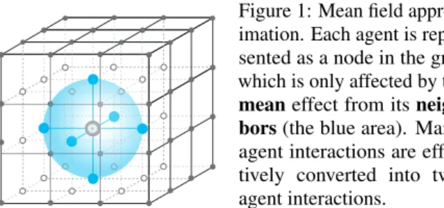
As illustrated in Fig. 1, with the mean field approxima-tion, the pairwise interactionsQj_(s,aj_,ak_{)between agent}

j and each neighboring agentk are simplified as that be-tweenj, thecentralagent, and the virtualmeanagent, that is abstracted by the mean effect of all neighbors within j’s neighborhood. The interaction is thus simplified and

Figure 1: Mean field approx-imation. Each agent is repre-sented as a node in the grid, which is only affected by the meaneffect from its neigh-bors(the blue area). Many-agent interactions are effec-tively converted into two-agent interactions.

expressed by the mean field Q-function Qj_(s,aj_,a¯j_{) in}

Eq. (8). During the learning phase, given an experience e= s,{ak_},{rj_},s0_{, the mean fieldQ-function is updated} in a recurrent manner as Qj t+1(s,a j ,a¯j ) = (1−α)Qj t(s,a j ,a¯j ) +α[rj +γvtj(s0)], (9)

whereαtdenotes the learning rate, anda¯jis the mean action

of all neighbors of agentjas defined in Eq. (6). The mean field value functionvtj(s0)for agentjat timetin Eq. (9) is

vtj(s0) = X aj πtj a j |s0_,¯aj Ea¯j_(a−j_)∼π−j t h Qj t s0,a j ,a¯ji , (10)

As shown in Eqs. (9) and (10), with the mean field approxi-mation, the MARL problem is converted into that of solving for the central agent j’s best responseπtj w.r.t. the mean

actiona¯j _{of allj’s neighbors, which represents the action}

distribution of all neighboring agents of the central agentj. We introduce an iterative procedure in computing the best responseπtj of each agent j. In the stage game{Qt}, the

mean actiona¯j _{of all j’s neighbors is first calculated by}

averaging the actionsak_{taken by j’sN}j_{neighbors from the}

policiesπk

t parametrized by their previous mean actionsa¯−k

¯ aj ₌ 1 Nj X k ak_{, a}k _∼πk t(·|s,a¯−k), (11) With eacha¯j_{calculated as in Eq. (11), the policyπ}j

t changes

consequently due to the dependence on the currenta¯j_{. The}

new Boltzmann policy is then determined for eachjthat πtj(aj|s,a¯j) = exp −βQj t(s,aj,a¯j) P aj0∈Ajexp −βQ j t(s,aj0,a¯j) . (12) By iterating Eqs. (11) and (12), the mean actionsa¯j_{and the}

corresponding policiesπtj for all agents improves

alterna-tively. In spite of lacking an intuitive impression of being stationary, in the following subsections, we will show that the mean actiona¯j _{will be equilibrated at an unique point}

after several iterations, and hence the policyπ_tjconverges. To distinguish from the Nash value function vNash_{(s) in}

Eq. (4), we denote the mean field value function in Eq. (10) asvMF_{(s) , [v}1_{(s), . . . ,v}N_{(s)]. With v}MF_{assembled, we}

now define the mean field operatorHMFin the form of

HMFQ(s,a) =Es0_∼pr(s,a) +γvMF(s0). (13)

In fact, we can prove thatHMF_{forms a contraction mapping;}

that is, one updatesQby iteratively applying the mean field operator HMF_{, the mean fieldQ-function will eventually}

3.2. Implementation

We can implement the mean fieldQ-function in Eq. (8) by universal function approximators such as neural networks, where theQ-function is parameterized with the weightsφ. The update rule in Eq. (9) can be reformulated as weights ad-justment. For off-policy learning, we exploit either standard Q-learning (Watkins & Dayan, 1992) for discrete action spaces or DPG (Silver et al., 2014) for continuous action spaces. Here we focus on the former, which we call MF-Q. In MF-Q, agent jis trained by minimizing the loss function

L(φj) = yj−Qφj(s,aj,a¯j) 2 , where yj _{= r}j _+γvMF φj −

(s0_{)is the target mean field value} calculated with the weightsφj₋. DifferentiatingL(φj_)gives

∇φjL(φj) =

yj₋Qφj(s,aj,a¯j)

∇φjQ_φj(s,aj,¯aj), (14)

which enables the gradient-based optimizers for training. Instead of setting up Boltzmann policy using theQ-function as in MF-Q, we can explicitly model the policy by neural networks with the weightsθ, which leads to the on-policy actor-critic method (Konda & Tsitsiklis, 2000) that we call MF-AC. The policy networkπθj,i.e.the actor, of MF-AC

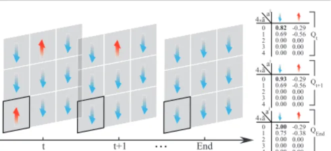
is trained by the sampled policy gradient: ∇θjJ(θj)≈ ∇_θjlogπ_θj(s)Q_φj(s,aj,a¯j) a=π_θj(s) . The critic of MF-AC follows the same setting for MF-Q with Eq. (14). During the training of MF-AC, one needs to alternatively updateφandθuntil convergence. We illustrate the MF-Qiterations in Fig. 2, and present the pesudocode for both MF-Qand MF-AC in Appendix A.

3.3. Proof of Convergence

We now prove the convergence ofQt ,[Q1t, . . . ,QtN]to the

NashQ-valueQ_∗= [Q1

∗, . . . ,Q∗N]as the iterations of MF-Q is applied. The proof is presented by showing that the mean field operatorHMF_{in Eq. (13) forms a contraction mapping}

with the fixed point atQ∗under the main assumptions. We start from introducing the assumptions:

Assumption 1. Each action-value pair is visited infinitely often, and the reward is bounded by some constant K. Assumption 2. Agent’s policy is Greedy in the Limit with Infinite Exploration (GLIE). In the case with the Boltzmann policy, the policy becomes greedyw.r.t. the Q-function in the limit as the temperature decays asymptotically to zero. Assumption 3. For each stage game[Q1

t(s), ...,QtN(s)]at

time t and in state s in training, for all t, s, j_{∈ {}1, . . . ,N_}, the Nash equilibriumπ_∗= [π1

∗, . . . , π∗N]is recognized either as 1) theglobal optimumor 2) asaddle pointexpressed as: 1. Eπ∗[Q j t(s)]≥Eπ[Qtj(s)], ∀π∈Ω Q kAk _; 2. Eπ_∗[Qtj(s)]≥EπjE π−j ∗ [Q j t(s)], ∀πj ∈Ω Aj and Eπ_∗[Qtj(s)]≤Eπ_∗jEπ−j[Q_tj(s)],∀π−j∈Ω Q k6=jAk . t t+1 End 4xāa j 0 1 2 3 4 0.82 0.69 0.00 0.00 0.00 -0.29 -0.56 0.00 0.00 0.00 aj 0 1 2 3 4 0.93 0.69 0.00 0.00 0.00 -0.29 -0.56 0.00 0.00 0.00 aj 0 1 2 3 4 2.00 0.75 0.00 0.00 0.00 -0.29 -0.38 0.00 0.00 0.00 Q_t Q_t+1 Q_End

...

Figure 2: MF-Qiterations on a3×3stateless toy example. The goal is to coordinate the agents to an agreed direction. Each agent has two choices of actions: up↑ ordown ↓. The reward of each agent’s staying in the same direction as its [0,1,2,3,4] neighbors are [−2.0,₋1.0,0.0,1.0,2.0], respectively. The neighbors are specified by the four direc-tions on the grid with cyclic structure on all direcdirec-tions,e.g. the first row and the third row are adjacent. The reward for the highlighted agentjon the bottom left at timet+ 1is2.0,

as all neighboring agents stay down in the same time. We listed the Q-tables for agentjat three time steps wherea¯j

is the percentage of neighboring ups. Following Eq. 9, we haveQj

t+1(↑,a¯j = 0) =Q

j

t(↑,a¯j= 0) +α[rj−Qtj(↑,a¯j =

0)] = 0.82 + 0.1×(2.0−0.82) = 0.93. The rightmost plot

shows the convergent scenario where theQ-value of staying down is2.0, which is the largest reward in the environment.

Note that Assumption 3 imposes a strong constraint on every single stage game encountered in training. In practice, how-ever, we find this constraint appears not to be a necessary condition for the learning algorithm to converge. This is in line with the empirical findings in Hu & Wellman (2003). Our proof is also built upon the two lemmas as follows: Lemma 1. Under Assumption 3, the Nash operatorHNash

in Eq.(4)forms a contraction mapping on the complete metric space from QtoQwith the fixed point being the

Nash Q-value of the entire game,i.e.HNash

t Q∗=Q∗. Proof. See Theorem 17 in Hu & Wellman (2003). Lemma 2. The random process{∆t}defined inRas

∆t+1(x) = (1−αt(x))∆t(x) +αt(x)Ft(x) (15)

converges to zero with probability1(w.p.1) when 1. 0≤αt(x)≤1,Ptαt(x) =∞,Ptα2t(x)<∞;

2. x∈X, the set of possible states, and|X|<_∞;

3. kE[Ft(x)|Ft]kW ≤ γk∆tkW+ct, whereγ∈[0,1)and

ctconverges to zerow.p.1;

4. var[Ft(x)|Ft]≤K(1 +k∆tk2W)with constant K>0.

HereFtdenotes the filtration of an increasing sequence of

σ-fields including the history of processes;αt, ∆t,Ft ∈Ft

andk · kWis a weighted maximum norm (Bertsekas, 2012).

Proof. See Theorem 1 in Jaakkola et al. (1994) and Corol-lary 5 Szepesvári & Littman (1999) for detailed derivation. We include it here to stay self-contained.

By subtractingQ_∗(s,a)on both sides of Eq. (9), we present the relation from the comparison with Eq. (15) such that

∆t(x) =Qt(s,a)−Q∗(s,a),

Ft(x) =rt+γvtMF(st+1)−Q∗(st,at), (16)

where x , (st,at)denotes the visited state-action pair at

timet. In Eq. (15),α(t)is interpreted as the learning rate

withαt(s0,a0) = 0for any(s0,a0)6= (st,at); this is because

that each agent only updates theQ-function with the statest

and actionsatvisited at timet. Lemma 2 suggests∆t(x)’s

convergence to zero, which means, if it holds, the sequence ofQ’s will asymptotically tend to the NashQ-valueQ_∗. One last piece to establish the main theorem is the below: Proposition 1. Let the metric space beRN_{and the metric}

be d(a,b) =P_j|aj_−bj_{|, fora= [a}j_]N

1,b= [bj]N1. If the

Q-function is K-Lipschitz continuousw.r.t.aj_{, then the}

op-eratorB(aj_),πj_(aj_|s,a¯j_{)in Eq.(12)forms a contraction}

mapping under sufficiently low temperatureβ. Proof. See details in Appendix D due to the space limit. Theorem 1. In a finite-state stochastic game, theQtvalues

computed by the update rule of MF-Q in Eq.(9)converges to the Nash Q-valueQ_∗= [Q1

∗, . . . ,Q∗N], if Assumptions 1, 2 & 3, and Lemma 2’s first and second conditions are met. Proof. LetFt denote theσ-field generated by all random

variables in the history of the stochastic game up to timet:

(st, αt,at,rt−1, ...,s1, α1,a1,Q0). Note thatQtis a random

variable derived from the historical trajectory up to timet. Given the fact that allQτ withτ < tare Ft-measurable,

both∆t andFt−1are therefore alsoFt-measurable, which

satisfies the measurability condition of Lemma 2.

To apply Lemma 2, we need to show that the mean field operatorHMFmeets Lemma 2’s third and fourth conditions.

For Lemma 2’s third condition, we begin with Eq. (16) that

Ft(st,at) =rt+γvtMF(st+1)−Q∗(st,at) =rt+γvNasht (st+1)−Q∗(st,at) +γ[vMF t (st+1)−vNasht (st+1)] =rt+γvNasht (st+1)−Q∗(st,at) +Ct(st,at) =FNash t (st,at) +Ct(st,at). (17)

Note the fact thatFNash

t in Eq. (17) is essentially theFt in

Lemma 2 in proving the convergence of the NashQ-learning algorithm. From Lemma 1, it is straightforward to show that

FNash

t forms a contraction mapping with the normk · k∞ being the maximum norm ona. We thus have for alltthat

kE[FNash

t (st,at)|Ft]k∞≤γkQt−Q∗k∞=γk∆tk∞. In meeting the third condition, we obtain from Eq. (17) that

kE[Ft(st,at)|Ft]k∞≤ kFtNash(st,at)|Ftk∞+kCt(st,at)|Ftk∞

≤γk∆tk∞+kCt(st,at)|Ftk∞. (18)

We are left to prove thatct =kCt(st,at)|Ftkconverges to

zerow.p.1. With Assumption 3, for each stage game, all the

globally optimal equilibrium(s) share the same Nash value, so does the saddle-point equilibrium(s). Each of the two following results is essentially associated with one of the two mutually exclusive scenarios in Assumption 3: 1. For globally optimal equilibriums, all players obtain the

joint maximum values that are unique and identical for all equilibriums according to the definition;

2. Suppose that the stage game{Qt}has two saddle-point

equilibriums,πandρ. It holds for agent jthat

EπjE_π−j[Q_tj(s)]≥E_ρjE_π−j[Q_tj(s)], EρjE_ρ−j[Q_tj(s)]≤E_ρjE_π−j[Q_tj(s)].

By combing the above inequalities, we obtain

EπjE_π−j[Q_tj(s)]≥E_ρjE_ρ−j[Q_tj(s)].

By the definition of saddle points, the above inequality still holds by reversing the order ofπandρ; hence, the equilibriums for agentiat both saddle points are the same such thatEπjE_π−j[Q_tj(s)] =E_ρjE_ρ−j[Q_tj(s)].

Given Proposition 1 that the policy based on the mean field Q-function forms a contraction mapping, and that all opti-mal/saddle points share the same Nash value in each stage game, with the homogeneity of agents,vMF_will

asymptoti-cally converges tovNash_{, the third condition is thus satisfied.}

For the fourth condition, we exploit the conclusion that is proved above thatHMFforms a contraction mapping, i.e.

HMF_Q

∗=Q∗, and it follows that

var[Ft(st,at)|Ft] =E[(rt+γvMFt (st+1)−Q∗(st,at))2]

=E[(rt+γvMFt (st+1)−HMF(Q∗))2]

=var[rt+γvtMF(st+1)|Ft]

≤K(1 +k∆tk2W). (19)

In the last step of Eq. (19), we employ Assumption 1 that the rewardrtis always bounded by some constant. Finally, with

all conditions met, it follows Lemma 2 that∆tconverges to

zerow.p.1,i.e.Qtconverges toQ∗w.p.1.

Apart from being convergent to the NashQ-value, MF-Qis alsoRational(Bowling & Veloso, 2001; 2002). We leave the corresponding discussion in Appendix D for details.

4. Related Work

We continue our discussion on related work from Intro-duction and make comparisons with existing techniques in a greater scope. Our work follows the same direction as Littman (1994); Hu & Wellman (2003); Bowling & Veloso (2002) on adapting a Stochastic Game (van der Wal et al., 1981) into the MARL formulation. Specifically, Littman (1994) addressed two-player zero-sum stochastic games by introducing a “minimax” operator inQ-learning, whereas Hu & Wellman (2003) extended it to the general-sum case

0 200 400 600 800 1000 Timestep 0.0 0.2 0.4 0.6 0.8 1.0 Performance IL FMQ Rec-FMQ MF-Q MAAC MF-AC (a)N= 100 0 200 400 600 800 1000 Timestep 0.0 0.2 0.4 0.6 0.8 1.0 Performance IL FMQ Rec-FMQ MF-Q MAAC MF-AC (b)N= 500 0 200 400 600 800 1000 Timestep 0.0 0.2 0.4 0.6 0.8 1.0 Performance IL FMQ Rec-FMQ MF-Q MAAC MF-AC (c)N= 1000

Figure 3: Learning withNagents in the GS environment withµ= 400andσ= 200. by learning a Nash equilibrium in each stage game and

con-sidering a mixed strategy. Nash-Q learning is guaranteed to converge to Nash strategies under the (strong) assumption that there exists an equilibrium for every stage game. In the situation where agents can be identified as either "friends" or "foes" (Littman, 2001), one can simply solve it by al-ternating between fully cooperative and zero-sum learning. Considering the convergence speed, Littman & Stone (2005) and de Cote & Littman (2008) draw on thefolk theoremand acquired a polynomial-time Nash equilibrium algorithm for repeated stochastic games, while Bowling & Veloso (2002) tried varying the learning rate to improve the convergence. The recent treatment of MARL was using deep neural net-works as the function approximator. In addressing the non-stationary issue in MARL, various solutions have been pro-posed including neural-based opponent modeling (He & Boyd-Graber, 2016), policy parameters sharing (Gupta et al., 2017),etc. Researchers have also adopted the paradigm of centralized training with decentralized executionfor multi-agent policy-gradient learning: BICNET (Peng et al., 2017), COMA (Foerster et al., 2018) and MADDPG (Lowe et al., 2017a), which allows the centralized criticQ-function to be trained with the actions of other agents, while the actor needs only local observation to optimize agent’s policy. The above MARL approaches limit their studies mostly to tens of agents. As the number of agents grows larger, not only the input space ofQ grows exponentially, but most critically, the accumulated noises by the exploratory actions of other agents make theQ-function learning no longer fea-sible. Our work addresses the issue by employing the mean field approximation (Stanley, 1971) over the joint action space. The parameters of theQ-function is independent of the number of agents as it transforms multiple agents inter-actions into two entities interinter-actions (single agentv.s.the distribution of the neighboring agents). This would effec-tively alleviate the problem of the exploratory noise (Colby et al., 2015) caused by many other agents, and allow each agent to determine which actions are beneficial to itself. Our work is also closely related to the recent development of mean field games (MFG) (Lasry & Lions, 2007; Huang et al., 2006; Weintraub et al., 2006). MFG studies popula-tion behaviors resulting from the aggregapopula-tions of decisions taken from individuals. Mathematically, the dynamics are governed by a set of two stochastic differential equations

that model the backward dynamics of individual’s value function, and the forward dynamics of the aggregate dis-tribution of agent population. Despite that the backward equation equivalently describes what Bellman equation in-dicates in the MDP, the primarily goal for MFG is rather for a model-based planning and to infer the movements of the individual density through time. The mean field approxima-tion (Stanley, 1971) in also employed in physics, but our work is different in that we focus on a model-free solution of learning optimal actions when the dynamics of the system and the reward function are unknown. Very recently, Yang et al. (2017) built a connection between MFG and reinforce-ment learning. Their focus is, however, on the inverse RL in order to learn both the reward function and the forward dynamics of the MFG from the policy data, whereas our goal is to form a computableQ-learning algorithm under the framework of temporal difference learning.

5. Experiments

We analyze and evaluate our algorithms in three different scenarios, including two stage games: the Gaussian Squeeze and the Ising Model, and themixed cooperative-competitive battle game.

5.1. Gaussian Squeeze

Environment.In the Gaussian Squeeze (GS) task (Holmes-Parker et al., 2014),Nhomogeneous agents determine their individual actionaj_{to jointly optimize the most}

appropri-ate summation x = PN_j=1aj_{. Each agent has 10 action}

choices – integers0to9. The system objective is defined asG(x) = xe−(xσ−2µ)2, where_µand_σare the pre-defined mean and variance of the system. In the scenario of traffic congestion, each agent is one traffic controller trying to send aj_{vehicles into the main road. Controllers are expected to}

coordinate with each other to make the full use of the main route while avoiding congestions. The goal of each agent is to learn to allocate system resources efficiently, avoiding either over-use or under-use. The GS problem here sits ideally as an ablation study on the impact of multi-agent exploratory noises toward the learning (Colby et al., 2015). Model Settings.We implement MF-Qand MF-AC follow-ing the framework of centralized trainfollow-ing (shared critic) with decentralized execution (independent actor). We compare

0.0 0.5 1.0 1.5 2.0 2.5 Temperature 0.0 0.2 0.4 0.6 0.8 1.0 Order Parameter MCMC MF-Q

Figure 4: Theorder parameterat equilibriumv.s. tempera-ture in the Ising model with20×20grid.

0 5000 10000 15000 20000 Timestep 0.0 0.2 0.4 0.6 0.8 1.0 Order Parameter OP 0.0 0.2 0.4 0.6 0.8 1.0

Mean Squared Error

MSE (a)τ= 0.8 0 5000 10000 15000 20000 Timestep 0.0 0.2 0.4 0.6 0.8 1.0 Order Parameter OP 0.0 0.2 0.4 0.6 0.8 1.0

Mean Squared Error

MSE

(b)τ= 1.2

Figure 5: Training performance of MF-Qin the Ising model with20×20grid.

against 4 baseline models: (1) Independent Learner (IL), a traditionalQ-Learning algorithm that does not consider the actions performed by other agents; (2) Frequency Max-imumQ-value (FMQ) (Kapetanakis & Kudenko, 2002), a modified IL which increases theQ-values of actions that frequently produced good rewards in the past; (3) Recursive Frequency MaximumQ-value (Rec-FMQ) (Matignon et al., 2012), an improved version of FMQ that recursively com-putes the occurrence frequency to evaluate and then choose actions; (4) Multi-agent Actor-Critic (MAAC), a variant of MADDPG architecture for the discrete action space (see Eq. (4) in Lowe et al. (2017b)). All models use the multi-layer perception as the function approximator. The detailed settings of the implementation are in the Appendix C.1. Results. Figure. 3 illustrates the results for the GS envi-ronment of µ = 400 and σ = 200 with three different numbers of agents (N = 100,500,1000) that stand for3

levels of congestions. In the smallest GS setting of Fig. 3a, all models show excellent performance. As the agent num-ber increases, Figs. 3b and 3c show MF-Qand MF-AC’s capabilities of learning the optimal allocation effectively after a few iterations, whereas all four baselines fail to learn at all. We believe this advantage is due to the awareness of other agents’ actions under the mean field framework; such mechanism keeps the interactions among agents man-ageable while reducing the noisy effect of the exploratory behaviors from the other agents. Between MF-Qand MF-AC, MF-Qconverges faster. Both FMQ and Rec-FMQ fail to reach pleasant performance, it might be because agents are essentially unable to distinguish the rewards received for the same actions, and are thus unable to update their own Q-valuesw.r.t.the actual contributions. It is worth noting that MAAC is surprisingly inefficient in learning when the number of agents becomes large; it simply fails to handle the non-aggregated noises due to the agents’ explorations.

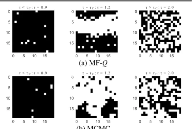
0 5 10 15 0 5 10 15 τ > τC: τ = 2 .0 0 5 10 15 0 5 10 15 τ τC: τ = 1 .2 0 5 10 15 0 5 10 15 τ < τC: τ = 0 .9 ~ (a) MF-Q 0 5 10 15 0 5 10 15 τ > τC: τ = 2 .0 0 5 10 15 0 5 10 15 τ τC: τ = 1 .2 0 5 10 15 0 5 10 15 τ < τC: τ = 0 .9 ~ (b) MCMC

Figure 6: The spins of the Ising model at equilibrium under different temperatures.

5.2. Model-free MARL for Ising Model

Environment. In statistical mechanics, the Ising model is a mathematical framework to describe ferromagnetism (Ising, 1925). It also has wide applications in sociophysics (Galam & Walliser, 2010). With the energy function explic-itly defined, mean field approximation (Stanley, 1971) is a typical way to solve the Ising model for every spinj,i.e. haj_i=P

aajP(a). See the Appendix C.2 for more details.

To fit into the MARL setting, we transform the Ising model into a stage game where the reward for each spin/agent is defined byrj _{= h}j_aj₊ λ

2

P

k∈N(j)ajak; hereN(j)is the

set of nearest neighbors of spinj,hj_{∈Ris the external field}

affecting the spinj, andλ_∈Ris an interaction coefficient that determines how much the spins are motivated to stay aligned. Unlike the typical setting in physics, here each spin does not know the energy function, but aims to understand the environment, and to maximize its reward by learning the optimal policy of choosing the spin state: up or down. In addition to the reward, theorder parameter(OP) (Stanley, 1971) is a traditional measure of purity for the Ising model.

OP is defined asξ = |N↑−N↓|

N , where N↑ represents the

number of up spins, andN↓for the down spins. The closer the OP is to1, the more orderly the system is.

Model Settings. To validate the correctness of the MF-Qlearning, we implement MCMC methods (Binder et al., 1993) to simulate the same Ising model and provide the ground truth for comparison. The full settings of MCMC and MF-Qfor Ising model are provided in the Appendix C.2. One of the learning goals is to obtain the accurate approximation ofhaj_{i. Notice that agents here do not know}

exactly the energy function, but rather use the temporal difference learning to approximatehaj_{iduring the learning}

procedure. Once this is accurately approximated, the Ising model as a whole should be able to converge to the same simulation result suggested by MCMC.

Correctness of MF-Q.Figure. 4 illustrates the relationship between the order parameter at equilibrium under different

Start

(a) Battle game scene.

0 250 500 750 1000 1250 1500 1750 2000 Epoch −800 −600 −400 −200 0 200 Reward MFAC MFQ (b) Learning curve. Figure 7: The battle game:64v.s.64.

system temperatures. MF-Qconverges nearly to the exact same plot as MCMC, this justifies the correctness of our algorithms. Critically, MF-Qfinds a similar Curie tempera-ture (the phase change point) as MCMC that isτ= 1.2. As

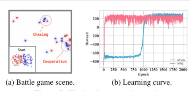
far as we know, this is the first work that manages to solve the Ising model via model-free reinforcement learning meth-ods. Figure. 5 illustrates the mean squared error between the learnedQ-value and the reward target. MF-Qis shown in Fig. 5a to be able to learn the target well under low temper-ature settings. When it comes to the Curie tempertemper-ature, the environment enters into the phase change when the stochas-ticity dominates, resulting in a lower OP and higher MSE observed in Fig. 5b. We visualize the equilibrium in Fig. 6. The equilibrium points from MF-Qin fact match MCMC’s results under three types of temperatures. The spins tend to stay aligned under a low temperature (τ= 0.9). As the temperature rises (τ = 1.2), some spins become volatile and patches start to form as spontaneous magnetization. This phenomenon is mostly observed around the Curie tem-perature. After passing the Curie temperature, the system becomes unstable and disordered due to the large thermal fluctuations, resulting in random spinning patterns. 5.3. Mixed Cooperative-Competitive Battle Game Environment. The Battle game in the Open-source MA-gent system (Zheng et al., 2018) is aMixed Cooperative-Competitivescenario with two armies fighting against each other in a grid world, each empowered by a different RL algorithm. In the setting of Fig. 7a, each army consists of

64homogeneous agents. The goal of each army is to get

more rewards by collaborating with teammates to destroy all the opponents. Agent can takes actions to either move to or attack nearby grids. Ideally, the agents army should learn skills such as chasing to hunt after training. We adopt the default reward setting:−0.005for every move,0.2for at-tacking an enemy,5for killing an enemy,−0.1for attacking an empty grid, and−0.1for being attacked or killed. Model Settings. Our MF-Q and MF-AC are compared against the baselines that are proved successful on the MA-gent platform. We focus on the battles between mean field methods (MF-Q, MF-AC) and their non-mean field counter-parts, independentQ-learning (IL) and advantageous actor critic (AC). We exclude MADDPG/MAAC as baselines, as the framework of centralized critic cannot deal with the varying number of agents for the battle (simply because

AC IL MF-Q MF-AC 0.0 0.2 0.4 0.6 0.8 1.0 1.2 1.4 Win-Rate vs IL vs MF-Q vs MF-ACvs AC

(a) Average wining rate.

AC IL MF-Q MF-AC 0 50 100 150 200 250 300 350 400 Total-Reward vs IL vs MF-Q vs MF-ACvs AC

(b) Average total reward. Figure 8: Performance comparisons in the battle game. agents could die in the battle). Also, as we demonstrated in the previous experiment of Fig. 3, MAAC tends to scale poorly and fail when the agent number is in hundreds. Results and Discussion.We train all four models by 2000 roundsself-plays, and then use them for comparative battles. During the training, agents can quickly pick up the skills of chasing and cooperation to kill in Fig. 7a. The Fig. 8 shows the result of winning rate and the total reward over 2000 rounds cross-comparative experiments. It is evident that on all the metrics mean field methods, MF-Qlargely outperforms the corresponding baselines,i.e.IL and AC re-spectively, which shows the effectiveness of the mean field MARL algorithms. Interestingly, IL performs far better than AC and MF-AC (2nd block from the left in Fig. 8a), although it is worse than the mean field counterpart MF-Q. This might imply the effectiveness of off-policy learning with shuffled buffer replay in many-agent RL towards a more stable learning process. Also, theQ-learning family tends to introduce a positive bias (Hasselt, 2010) by using the maximum action value as an approximation for the max-imum expected action value, and such overestimation can be beneficial for each single agent to find the best response to others even though the environment itself is still changing. On the other hand, On-policy methods need to comply with the GLIE assumption (Assumption 2 in Sec 3.3) so as to converge properly to the optimal value (Singh et al., 2000), which is in the end a greedy policy as off-policy methods. Figure. 7b further shows the self-play learning curves of MF-AC and MF-Q. MF-Q presents a faster convergence speed than MF-AC, which is consistent with the findings in the Gaussian Squeeze task (see Fig. 3b & 3c). Apart from 64, we further test the scenarios when the agent size is 8, 144, 256, the comparative results keep the same relativity as

Fig. 8; we omit the presentations for clarity.

6. Conclusions

In this paper, we developed mean field reinforcement learn-ing methods to model the dynamics of interactions in the multi-agent systems. MF-Qiteratively learns each agent’s best response to the mean effect from its neighbors; this ef-fectively transform the many-body problem into a two-body problem. Theoretical analysis on the convergence of the MF-Qalgorithm to NashQ-value was provided. Three types of tasks have justified the effectiveness of our approaches. In particular, we report the first result to solve the Ising model using model-free reinforcement learning methods.

Acknowledgement

We sincerely thank Ms. Yi Qu for her generous help on the graphic design.

References

Bertsekas, D. P. Weighted sup-norm contractions in dynamic programming: A review and some new applications.Dept. Elect. Eng. Comput. Sci., Massachusetts Inst. Technol., Cambridge, MA, USA, Tech. Rep. LIDS-P-2884, 2012. Binder, K., Heermann, D., Roelofs, L., Mallinckrodt, A. J.,

and McKay, S. Monte carlo simulation in statistical physics. Computers in Physics, 7(2):156–157, 1993. Blume, L. E. The statistical mechanics of strategic

inter-action. Games and economic behavior, 5(3):387–424, 1993.

Bowling, M. and Veloso, M. Rational and convergent learn-ing in stochastic games. InInternational joint confer-ence on artificial intelligconfer-ence, volume 17, pp. 1021–1026. Lawrence Erlbaum Associates Ltd, 2001.

Bowling, M. and Veloso, M. Multiagent learning using a variable learning rate. Artificial Intelligence, 136(2): 215–250, 2002.

Busoniu, L., Babuska, R., and De Schutter, B. A com-prehensive survey of multiagent reinforcement learning. IEEE Trans. Systems, Man, and Cybernetics, Part C, 38 (2):156–172, 2008.

Cao, Z., Qin, T., Liu, T.-Y., Tsai, M.-F., and Li, H. Learning to rank: from pairwise approach to listwise approach. InProceedings of the 24th international conference on Machine learning, pp. 129–136. ACM, 2007.

Colby, M. K., Kharaghani, S., HolmesParker, C., and Tumer, K. Counterfactual exploration for improving multiagent learning. InProceedings of the 2015 International Con-ference on Autonomous Agents and Multiagent Systems, pp. 171–179. International Foundation for Autonomous Agents and Multiagent Systems, 2015.

de Cote, E. M. and Littman, M. L. A polynomial-time nash equilibrium algorithm for repeated stochastic games. In McAllester, D. A. and Myllymäki, P. (eds.),UAI 2008, pp. 419–426. AUAI Press, 2008. ISBN 0-9749039-4-9. Fink, A. M. et al. Equilibrium in a stochasticn-person game.

Journal of science of the hiroshima university, series ai (mathematics), 28(1):89–93, 1964.

Foerster, J. N., Chen, R. Y., Al-Shedivat, M., Whiteson, S., Abbeel, P., and Mordatch, I. Learning with opponent-learning awareness. CoRR, abs/1709.04326, 2017.

Foerster, J. N., Farquhar, G., Afouras, T., Nardelli, N., and Whiteson, S. Counterfactual multi-agent policy gradients. In McIlraith & Weinberger (2018).

Galam, S. and Walliser, B. Ising model versus normal form game. Physica A: Statistical Mechanics and its Applications, 389(3):481–489, 2010.

Gupta, J. K., Egorov, M., and Kochenderfer, M. Cooperative multi-agent control using deep reinforcement learning. In AAMAS, pp. 66–83. Springer, 2017.

Hasselt, H. V. Double q-learning. InNIPS, pp. 2613–2621, 2010.

He, H. and Boyd-Graber, J. L. Opponent modeling in deep reinforcement learning. In Balcan, M. and Wein-berger, K. Q. (eds.),ICML, volume 48, pp. 1804–1813. JMLR.org, 2016.

HolmesParker, C., Taylor, M., Zhan, Y., and Tumer, K. Exploiting structure and agent-centric rewards to promote coordination in large multiagent systems. InAdaptive and Learning Agents Workshop, 2014.

Hu, J. and Wellman, M. P. Nash q-learning for general-sum stochastic games.Journal of machine learning research, 4(Nov):1039–1069, 2003.

Huang, M., Malhamé, R. P., Caines, P. E., et al. Large pop-ulation stochastic dynamic games: closed-loop mckean-vlasov systems and the nash certainty equivalence prin-ciple. Communications in Information & Systems, 6(3): 221–252, 2006.

Ising, E. Beitrag zur theorie des ferromagnetismus. Zeitschrift für Physik, 31(1):253–258, 1925.

Jaakkola, T., Jordan, M. I., and Singh, S. P. Convergence of stochastic iterative dynamic programming algorithms. In NIPS, pp. 703–710, 1994.

Jeong, S. H., Kang, A. R., and Kim, H. K. Analysis of game bot’s behavioral characteristics in social interaction networks of mmorpg. InACM SIGCOMM Computer Communication Review, volume 45, pp. 99–100. ACM, 2015.

Kapetanakis, S. and Kudenko, D. Reinforcement learning of coordination in cooperative multi-agent systems. In NCAI, pp. 326–331, Menlo Park, CA, USA, 2002. ISBN 0-262-51129-0.

Konda, V. R. and Tsitsiklis, J. N. Actor-critic algorithms. In Solla, S. A., Leen, T. K., and Müller, K. (eds.),Advances in Neural Information Processing Systems 12, pp. 1008– 1014. MIT Press, 2000.

Kreyszig, E.Introductory functional analysis with applica-tions, volume 1. wiley New York, 1978.

Lasry, J.-M. and Lions, P.-L. Mean field games.Japanese journal of mathematics, 2(1):229–260, 2007.

Lemke, C. E. and Howson, Jr, J. T. Equilibrium points of bimatrix games.Journal of the Society for Industrial and Applied Mathematics, 12(2):413–423, 1964.

Littman, M. L. Markov games as a framework for multi-agent reinforcement learning. InICML, volume 157, pp. 157–163, 1994.

Littman, M. L. Friend-or-foe q-learning in general-sum games. InICML, volume 1, pp. 322–328, 2001.

Littman, M. L. and Stone, P. A polynomial-time nash equi-librium algorithm for repeated games.Decision Support Systems, 39(1):55–66, 2005.

Lowe, R., Wu, Y., Tamar, A., Harb, J., Abbeel, O. P., and Mordatch, I. Multi-agent actor-critic for mixed cooperative-competitive environments. InNIPS, pp. 6382– 6393, 2017a.

Lowe, R., Wu, Y., Tamar, A., Harb, J., Abbeel, P., and Mor-datch, I. Multi-agent actor-critic for mixed cooperative-competitive environments. In Guyon, I., von Luxburg, U., Bengio, S., Wallach, H. M., Fergus, R., Vishwanathan, S. V. N., and Garnett, R. (eds.),NIPS, pp. 6382–6393, 2017b.

Matignon, L., Laurent, G. J., and Le Fort-Piat, N. Inde-pendent reinforcement learners in cooperative markov games: a survey regarding coordination problems. The Knowledge Engineering Review, 27(1):1–31, 2012. McIlraith, S. A. and Weinberger, K. Q. (eds.).Proceedings

of the Thirty-Second AAAI Conference on Artificial In-telligence, New Orleans, Louisiana, USA, February 2-7, 2018, 2018. AAAI Press.

Panait, L. and Luke, S. Cooperative multi-agent learning: The state of the art.AAMAS, 11(3):387–434, 2005. Peng, P., Yuan, Q., Wen, Y., Yang, Y., Tang, Z., Long,

H., and Wang, J. Multiagent bidirectionally-coordinated nets for learning to play starcraft combat games.CoRR, abs/1703.10069, 2017.

Rendle, S. Factorization machines with libfm.ACM Trans-actions on Intelligent Systems and Technology (TIST), 3 (3):57, 2012.

Shapley, L. S. Stochastic games.Proceedings of the national academy of sciences, 39(10):1095–1100, 1953.

Silver, D., Lever, G., Heess, N., Degris, T., Wierstra, D., and Riedmiller, M. Deterministic policy gradient algorithms. InICML, pp. 387–395, 2014.

Singh, S., Jaakkola, T., Littman, M. L., and Szepesvári, C. Convergence results for single-step on-policy reinforcement-learning algorithms. Machine learning, 38(3):287–308, 2000.

Stanley, H. E. Phase transitions and critical phenomena. Clarendon, Oxford, 9, 1971.

Szepesvári, C. and Littman, M. L. A unified analysis of value-function-based reinforcement-learning algorithms. Neural computation, 11(8):2017–2060, 1999.

Tan, M. Multi-agent reinforcement learning: Independent vs. cooperative agents. InProceedings of the tenth inter-national conference on machine learning, pp. 330–337, 1993.

Troy, C. A. Envisioning stock trading where the brokers are bots.New York Times, 16, 1997.

van der Wal, J., van der Wal, J., van der Wal, J., Math-ématicien, P.-B., van der Wal, J., and Mathematician, N. Stochastic Dynamic Programming: successive ap-proximations and nearly optimal strategies for Markov decision processes and Markov games. Mathematisch centrum, 1981.

Wang, J., Zhang, W., Yuan, S., et al. Display advertising with real-time bidding (rtb) and behavioural targeting. Foundations and TrendsR in Information Retrieval, 11 (4-5):297–435, 2017.

Watkins, C. J. and Dayan, P. Q-learning.Machine learning, 8(3-4):279–292, 1992.

Weintraub, G. Y., Benkard, L., and Van Roy, B. Oblivious equilibrium: A mean field approximation for large-scale dynamic games. InAdvances in neural information pro-cessing systems, pp. 1489–1496, 2006.

Yang, J., Ye, X., Trivedi, R., Xu, H., and Zha, H. Deep mean field games for learning optimal behavior policy of large populations.CoRR, abs/1711.03156, 2017. Zheng, L., Yang, J., Cai, H., Zhou, M., Zhang, W., Wang, J.,

and Yu, Y. Magent: A many-agent reinforcement learning platform for artificial collective intelligence. In McIlraith & Weinberger (2018).

A. Detailed mean field reinforcement learning algorithms

InitialiseQφj,Q

φ₋j , anda¯jfor all j∈ {1, . . . ,N}

whiletraining not finisheddo form= 1, ...,Mdo

For each agentj, sample actionaj_fromQ

φj by Eq. (12), with the current mean actiona¯jand the exploration rateβ

For each agent j, compute the new mean actiona¯j_{by Eq. (11)}

Take the joint actiona= [a1_{, . . . ,a}N_{]and observe the rewardr= [r}1_{, . . . ,r}N_{]and the next states}0 Storehs,a,r,s0_{,a¯iin replay bufferD, wherea¯= [¯a}1_{, . . . ,a¯}N_]

forj= 1toNdo

Sample a minibatch ofKexperienceshs,a,r,s0,a¯ifromD

Sample actionaj −fromQφj −witha¯ j −←a¯j Setyj _=rj_+γvMF φ₋j (s0)by Eq. (10)

Update theQ-network by minimizing the lossL(φj_{) =} 1 K

P

yj_−Q

φj(sj,aj,a¯j)2

Update the parameters of the target network for each agentjwith learning rateτ: φ₋j _←τφj_{+ (1−τ)φ}j

− Algorithm 2Mean Field Actor-Critic (MF-AC)

InitializeQφj,Q

φ₋j ,πθj,π

θ₋j , anda¯jfor allj∈ {1, . . . ,N}

whiletraining not finisheddo

For each agentj, sample actionaj _=π

θj(s); compute the new mean actiona¯= [¯a1, . . . ,a¯N]

Take the joint actiona= [a1_{, . . . ,a}N_{]and observe the rewardr= [r}1_{, . . . ,r}N_{]and the next states}0 Storehs,a,r,s0_{,a¯iin replay bufferD}

forj= 1toNdo

Sample a minibatch ofKexperienceshs,a,r,s0_,a¯ifromD Setyj _=rj_+γvMF

φ₋j (s0)by Eq. (10)

Update the critic by minimizing the lossL(φj_{) =} 1 K

P

yj_−Q

φj(s,aj,a¯j)2

Update the actor using the sampled policy gradient: ∇θjJ(θj)≈ 1 K X ∇θjlogπ_θj(s0)Q φ₋j (s0,a j −,a¯ j −) a₋j=π_θj − (s0)

Update the parameters of the target networks for each agentjwith learning ratesτφandτθ:

φ₋j ←τφφj+ (1−τφ)φ₋j

B. Proof of the bound for the remainder term in Eq. 7

Recall Eq. (8) that we approximate the actionak_{taken by the neighboring agentkwith the mean actiona¯calculated from}

the neighborhoodN(j). The statesand the actionaj of the central agentjcan be considered as fixed parameters; the

indicesj,kof agents are essentially irrelevant to the derivation. With those omitted for simplicity, We rewrite the expression of the pairwiseQ-function asQ(a),Qj_(s,aj_,ak_).

Suppose thatQisM-smooth, where its gradient∇Qis Lipschitz-continuous with constantMsuch that for alla,a¯

k∇Q(a)− ∇Q(¯a)k2≤Mka−a¯k2, (20)

wherek · k2indicates the`2-norm.

With the Lagrange’s mean value theorem, we have

∇Q(a)− ∇Q(¯a) =∇Q(¯a+ 1·(a−a¯))− ∇Q(¯a) =∇2_{Q(¯a+·(a−a¯))·(a−a¯), where ∈[0,1]. (21)}

Take the`2-norm on the both sides of the above equation, it follows from the smoothness condition that

k∇Q(a)− ∇Q(¯a)k2=k∇2Q(¯a+τ·(a−a¯))·(a−a¯)k2≤Mka−a¯k2. (22)

Defineδa,a−a¯and the normalized vectorδaˆ,a−¯a_{/ka−a¯k2withkδaˆk}

2= 1, it follows from the above inequality

k∇2_{Q(a+τ·δa)·δaˆk}

2≤M. (23)

By arbitrary choice of (the unnormalized vector)δasuch that the magnitudekδak2→0, it follows from above that

k∇2_Q(a)·δaˆk

2≤M. (24)

By aligning (the normalized vector)δaˆin the direction of the eigenvectors of the Hessian matrix∇2_{Q, we can obtain for}

any eigenvalueλof∇2_Qthat

k∇2_Q(a)·δaˆk

2=kλ·δaˆk2=|λ| · kδaˆk2≤M, (25)

which indicates that all eigenvalues of∇2_{Qcan be bounded in the symmetric interval[−M,M].}

As the Hessian matrix∇2_{Qis real symmetric and hence diagonalizable, there exist an orthogonal matrixU such that}

U>_[∇2_{Q]U=Λ,diag[λ}

1, . . . , λD]. It then follows that

δa_{· ∇}2_Q

·δa= [Uδa]>Λ[Uδa] =

D

X

i=1

λi[Uδa]2i, with −MkUδak2≤ D

X

i=1

λi[Uδa]2i ≤MkUδak2 (26)

Recall the definitionδa = a−a¯in Eq. (6), whereais the one-hot encoding forD actions, anda¯is aD-dimensional multinomial distribution. It can be shown that

kUδak2=kδak2= (a−a¯)>(a−a¯) =a>a+ ¯a>a¯−a¯>a−a>a¯= 2(1−a¯i)≤2, (27)

whereirepresents the specific actionahas represented such thatai0 = 0fori06=i.

With all elements assembled, we have proved that each single remainder termRj

C. Experiment details

IL, FMQ, Rec-FMQ and MF-Qall use a three-layer MLP to approximateQ-value. All agents share the sameQ-network for each experiment. The sharedQ-network takes an agent embedding as input and computesQ-value for each candidate action. For MF-Q, we also feed in the action approximation a¯. We use the Adam optimizer with a learning rate of 0.00001 and-greedy exploration unless otherwise specified. For FMQ, we set the exponential decay rates= 0.006, start

temperaturemax_temp=1000and FMQ heuristicc= 5. For Rec-FMQ, we set the frequency learning rateαf = 0.01.

MAAC and MF-ACuse the Adam optimizer with a learning rate of 0.001 and 0.0001 for Critics and Actors respectively, andτ= 0.01for updating the target networks. We share the Critic among all agents in each experiment and feed in an agent embedding as extra input. Actors are kept separate. The discounted factorγis set to be 0.95 and the mini-batch size is set to be 200. The size of the replay buffer is106_{and we update the network parameters after every 500 samples added to the}

replay buffer.

For all models, we use the performance of the joint-policy learned up to that point if learning and exploration were turned off (i.e., take the greedy action w.r.t. the learned policy) to compare our method with the above baseline models.

C.2. Ising Model

An Ising model is defined as a stateless system withNhomogeneous sites on a finite square lattice. Each site determines their individual spinaj _{to interact with each other and aims to minimize the system energy for a more stable environment.}

The system energy is defined as

E(a,h) =−X j (hjaj+λ 2 X k∈N(j) aj_ak_{) (28)}

whereN(j)is the set of nearest neighbors of sitej,hj_{∈Ris the external field affecting sitej, andλ∈Ris an interaction}

term determines how much the sites tend to align in the same direction. The system is said to reach an equilibrium point when the system energy is minimized, with the probability

P(a) = Pexp (−E(a,h)/τ)

aexp(−E(a,h)/τ)

, (29)

whereτis the system temperature. When the temperature rises beyond a certain point (the Curie temperature), the system can no longer keep a stable form and a phase transition happens. As the ground-truth is known, we would be able to evaluate the correctness of theQ-function learning when there is a large body of agents interacted.

The mean field theory provides an approximate solution tohaj_i=P

aajP(a)through a set of self-consistent mean field

equations haj i= exp −[hj_aj_+λP k∈N(j)haki]/τ 1 + exp−[hj_aj_+λP k∈N(j)haki]/τ . (30)

which can be solved iteratively by haj i(t+1)= exp −[hj_aj_+λP k∈N(j)haki(t)]/τ 1 + exp−[hj_aj_+λP k∈N(j)haki(t)]/τ , (31)

wheretrepresents the number of iterations.

To learn an optimal joint policyπ∗_{for Ising model, we use the statelessQ-learning with mean field approximation (MF-Q),} defined as

Qj_(aj_,a¯j₎

←Qj_(aj_,a¯j_{) +α[r}j

Algorithm 3MCMC in Ising Model

initialize spin statea∈ {−1,1}N_forNsites

whiletraining not finisheddo randomly choose sitej∈N(j)

flip the spin state for sitej:aj

−← −aj

compute neighbor energyE(a,h) =−Pj(hjaj+λ2

P k∈N(j)ajak)forajanda j − randomly choose_∼U(0,1) ifexp((E(aj_,h)−E(aj −,h))/τ)> then aj _←aj −

where the meana¯j_{is given as the meanha}j_{ifrom the last time step, and the individual reward is}

rj_=hj_aj₊λ

2

X

k∈N(j)

aj_ak_{. (33)}

To balance the trade-off between exploration and exploitation under low temperature settings, we use a policy with Boltzmann exploration and a decayed exploring temperature. The temperature for Boltzmann exploration of MF-Qis multiplied by a decay factor exponentially through out the training process.

Without lost of generality, we assumeλ >0, thus neighboring sites with the same action result in lower energy (observe

higher reward) and are more stable. Each site should also align with the sign of external fieldhj_{to reduce the system energy.}

For simplification, we eliminate the effect of external fields and assume the model to be discrete,i.e.,∀j∈N,hj_{= 0,a}j_∈

{−1,1}.

We simulate the Ising model using Metropolis Monte Carlo methods (MCMC). After initialization, we randomly change a site’s spin state and calculate the energy change, select a random number between 0 and 1, and accept the state change only if the number is less thane(E j−E

j

−)

τ . This is called the Metropolis technique, which saves computation time by selecting the more probable spin states.

C.3. Battle Game

IL and MF-Q have almost the same hyper-parameters settings. The learning rate isα = 10−4_{, and with a dynamic}

exploration rate linearly decays fromγ= 1.0toγ= 0.05during the 2000 rounds training. The discounted factorγis set to be 0.95 and the mini-batch size is 128. The size of replay buffer is5×105_.

AC and MF-ACalso have almost the same hyper-parameters settings. The learning rate isα= 10−4_{, the temperature of}

soft-max layer inactorisτ= 0.1. And the coefficient of entropy in the total loss is 0.08, the coefficient of value in the total

D. Further details towards the theoretical guarantee of MF-

Q

Proposition 1. Let the metric space beRN _{and the metric be d(a,b) =}P

j|aj−bj|, for a= [aj]1N,b= [bj]N1. If the

Q-function is K-Lipschitz continuousw.r.t. aj_{, then the operatorB(a}j_{), π}j_(aj_|s,a¯j_{)in Eq.(12)forms a contraction}

mapping under sufficiently low temperatureβ.

Proof. Following the contraction mapping theorem (Kreyszig, 1978), in order to be a contraction, the operator has to satisfy: d(B(a),B(b))≤αd(a,b), ∀a,b

where0≤α <1andB(a),[B(a1_{), . . . ,B(a}N_)].

Here we start from binomial case and then adapt to the multinomial case in general. We first rewriteB(aj_)as

B(aj_{) =π}j_(aj |s,a¯j_{) =} exp −βQ j t(s,aj,a¯j) exp −βQj t(s,aj,a¯j) + exp −βQj t(s,¬aj,a¯j) = 1 1 + exp (−β_·∆Q(s,aj_,a¯)), (34) where∆Q(s,aj_{,a¯) =Q(s,a}¬j_{,a¯)−Q(s,a}j_,a¯). Then we have |B(aj₎ −B(bj₎ |= _{1 +e}−β·1∆Q(s,aj_,¯a)− 1 1 +e−β·∆Q(s,bj_,¯a) = βe −β∆Q0 (1 +e−β∆Q0₎2 ∆Q(s,aj,a¯)−∆Q(s,bj,a¯) ≤₄1_T ·Q(s,a¬j,a¯)−Q(s,b¬j,a¯) +Q(s,bj,a¯)−Q(s,aj,a¯) ≤₄1_T · K·1−aj_−(1−bj_)+K·aj_−bj ≤₄1_T ·2K·X j aj_−bj _{. (35)}

In the second equation, we apply the mean value theorem in calculus:∃x0∈[x1,x2],s.t., f(x1)− f(x2) = f0(x0)(x1−x2).

In the third equation we use the maximum value fore−β∆Q0_{/(1 +}e−β∆Q0₎2_{= 1/4}whenQ

0= 0. In the last equation we

apply the Lipschitz constraint in the assumption where constantK≥0. Finally, we have:

d(B(a),B(b))≤ 1 4T ·2K· X j aj_−bj = K 2Td(a,b) (36)

In order for the contraction to hold,T > K₂. In other words, when the action space is binary for each agent, and the temperature is sufficiently large, the mean field procedure converges.

This proposition can be easily extended to multinomial case by replacing binary variableaj_{by a multi-dimensional binary}

indicator vectoraj_{, on each dimension, the rest of the derivations would remain essentially the same.}

D.1. Discussion on Rationality

In line with (Bowling & Veloso, 2001; 2002), we argue that to better evaluate a multi-agent learning algorithm, on top of the convergence guarantee, discussion on property of Rationality is also needed.

Property 1. (also see (Bowling & Veloso, 2001; 2002)) In an N-agent stochastic game defined in this paper, given all agents converge to stationary policies, if the learning algorithm converges to a policy that is abest responseto the other agents’ policies, then the algorithm is Rationale.

Our mean fieldQ-learning is rational in that Eq. (5) converts many agents interactions into two-body interactions between a single agent and the distribution of other agents actions. When all agents follow stationary policies, their policy distribution would be stationary too. As such the two-body stochastic game becomes an MDP, and the agent would choose a policy (based on Assumption 2) which is the best response to the distribution of other stationary policies. As agents are symmetric in our case, they all show the best response to the distributions, and are therefore rational.