Deformable Object Manipulation: Learning While Doing

(1)

Deformable Object Manipulation:

Learning While Doing

by

Dale Mc_Conachie

A dissertation submitted in partial fulfillment of the requirements for the degree of

Doctor of Philosophy (Robotics)

in The University of Michigan 2020

Doctoral Committee:

Associate Professor Dmitry Berenson, Chair Professor Jessie Grizzle

Associate Professor Chad Jenkins

(2)

Dale Mc_Conachie [email protected] ORCID iD: 0000-0002-2615-3473

c

(3)

ACKNOWLEDGEMENTS

Thanks to Calder Phillips-Grafflin, Brad Saund, Andrew Dobson, and Yu-Chi Lin for helpful discussions. Thank you to all my collaborators from the Autonomous Robotic Manipulation Lab. Thanks to my advisor Dmitry Berenson for his guidance and encouragement. Thanks to Chad Jenkins, Jessie Grizzle, and Leslie Pack Kaelbling for their advice. Thanks to my parents for supporting my return to university and advice throughout. Finally, special thanks to my wife Molly for everything.

(4)

LIST OF FIGURES

Figure

3.1 Euclidean distance measures length of the shortest path between pi

and pj in R3 (gold). Geodesic distance measures the length of the

shortest path, constrained to stay within the deformable object (red). 13 3.2 An illustrative example of directional rigidity. Left: The rope moves

almost rigidly when dragging it by one end to the left. Right: The rope deforms when pulling it on the right in the opposite direction. 15 3.3 The length of the the red segment on the rope is the geodesic distance

Dij. vij is the vector showing the relative position of pj with respect

topi. . . 17

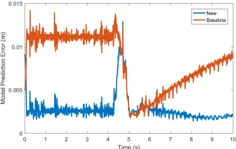
3.4 Projection process for points that are predicted to be in collision after movement. . . 20 3.5 RMS model prediction error for the simulated rope model accuracy

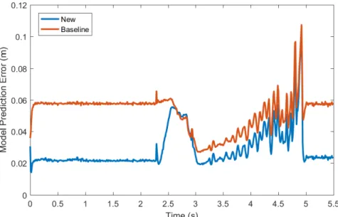
test. The gripper pulls the rope for the first 4.5 seconds, then turns for half a second, then moves in the opposite direction at the 5 second mark. . . 21 3.6 RMS model prediction error for the simulated cloth model accuracy

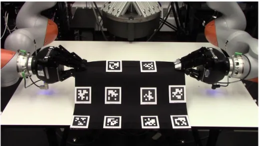
test. The grippers pull the cloth for the first 2.3 seconds, then turn for 0.63 seconds, then move in the opposite direction at the 2.93 second mark. At the 5 second mark the cloth is no longer folded. . . 22 3.7 Initial setup for the physical robot model accuracy experiment. . . . 23 3.8 RMS model prediction error for the physical cloth accuracy test. The

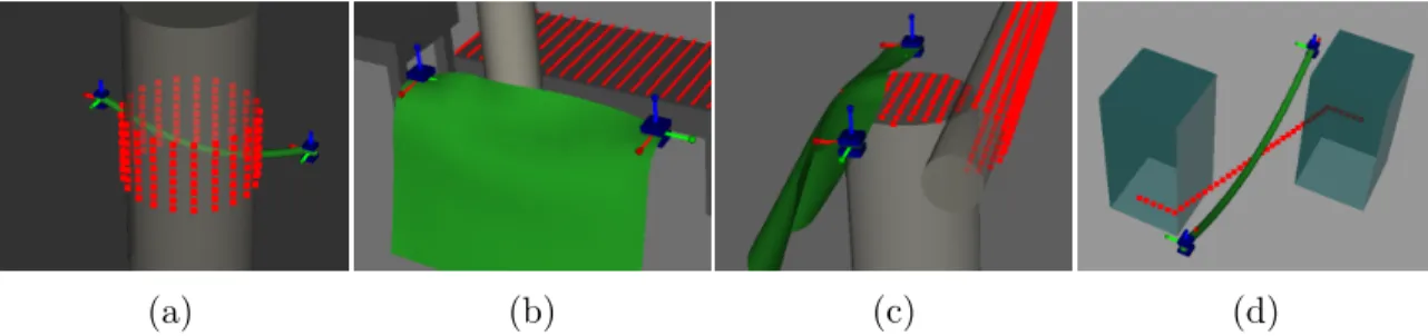
grippers pull the cloth toward the robot for the first 10 timesteps, upward for 5 timesteps, rotate for 15 timesteps, diagonally down and away for 9 timesteps, then directly away from the robot. . . 23 3.9 Initial state of the four experiments, where the red points act as

attractors for the deformable object. (a) Rope wrapping cylinder. (b) Cloth passing single pole. (c) Cloth covering two cylinders. (d) Rope matching zig-path . . . 24 4.1 Top Line: moving the point does not change the error, thus the

desired movement is zero, however, it is not important to achieve zero movement, thus Wd = 0. Bottom Line: error is at a local minimum;

(8)

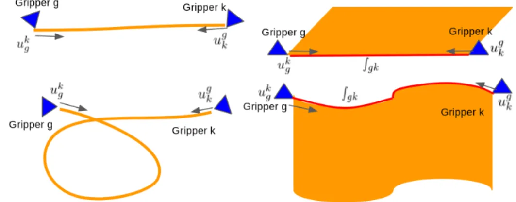
4.2 The arrows in gray show the direction of each stretching vector at the corresponding gripper with respect to the gripper pairqgandqk. Left:

stretching vectors on the rope when the rope is at rest (above) or is deformed (below). Right: stretching vectors on the cloth when the cloth is at rest (above) or is deformed (below). The red lines denote the geodesic connecting the corresponding pIg(qg,qk) and pIk(qg,qk) on the object. . . 33 4.3 Initial state of the four experiments, where the red points act as

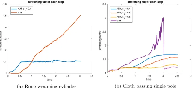
attractors for the deformable object. (a) Rope wrapping cylinder. (b) Cloth passing single pole. (c) Cloth covering two cylinders. (d) Rope matching zig-path . . . 36 4.4 (a) The red line shows theγof the benchmark and the blue line shows

the γ of the new controller with ss = 0.4 throughout the simulation.

(b) The purple line shows theγ of the benchmark, and the blue, red, and yellow lines each show theγ of the new controller withss= 0.4,

ss = 0.6, and ss = 0.8, respectively. . . 37

4.5 Cloth-covering-two-cylinder task start and end configurations. Both controllers are unable to make progress due to a local minima. . . . 37 4.6 Rope-matching-zig-path start and end configurations. Both

con-trollers are able to succeed at the task, bringing the rope into align-ment with the desired path. . . 38 4.7 Initial setup for the physical robot stretching avoidance test. . . 38 5.1 Sequence of snapshots showing the execution of the simulated

exper-iments using the KF-MANDB algorithm. The rope and cloth are shown in green, the grippers is shown in blue, and the target points are shown in red. The bottom row additionally shows ˙Pd as green

rays with red tips. . . 50 5.2 Experimental results for the rope-winding task. Top left: alignment

error for 10 trials for each MAB algorithm, and each model in the model set when used in isolation. UCB1-Normal, MANB, KF-MANDB lines overlap in the figure for all trials. Top right: Total regret averaged across 10 trials for each MAB algorithm with the minimum and maximum drawn in dashed lines. Bottom row: his-tograms of the number of times each model was selected by each MAB algorithm; UCB1-Normal (bl), KF-MANB (bm), KF-MANDB (br). . . 52 5.3 Experimental results for the table coverage task. See Figure 5.2 for

description. . . 53 5.4 Experimental results for the two-part coverage task. See Figure 5.2

(9)

6.1 Four example manipulation tasks for our framework. In the first two tasks, the objective is to cover the surface of the table (indicated by the red lines) with the cloth (shown in green). In the first task, the grippers (shown in blue) can freely move however the cloth is obstructed by a pillar. In the second task, the grippers must pass through a narrow passage before the table can be covered. In the third task, the robot must navigate a rope (shown in green in the top left corner) through a three-dimensional maze before covering the red points in the top right corner. The maze consists of top and bottom layers (purple and green, respectively). The rope starts in the bottom layer and must move to the target on the top layer through an opening (bottom left or bottom right). For the fourth task, the physical robot must move the cloth from the far side of an obstacle to the region marked in pink near the base of the robot. . . 56 6.2 Block diagram showing the major components of our framework. On

each cycle we use either the local controller (dotted purple arrows) or a planned path (dashed red arrows) to predict if the system will be deadlocked in the future, planning a new path is needed to avoid deadlock. . . 59 6.3 Motivating example for deadlock prediction. The local controller

moves the grippers on opposite sides of an obstacle, while the geodesic between the grippers (red line) cannot move past the pole, eventually leading to overstretch or tearing of the deformable object if the robot does not stop moving towards the goal. . . 60 6.4 Example of estimating the gross motion of the deformable object

for a prediction horizon Np = 10. The magenta lines start from

the points of the deformable object that are closest to the target points (according to the navigation function). These lines show the paths those points would follow to reach the target when following the navigation function. . . 64 6.5 Estimated gross motion of the deformable object (magenta lines) and

end effectors (blue spheres). The VEB (black lines) is forward prop-agated by tracking the end effector positions, changing to cyan lines when overstretch is predicted. . . 65 6.6 Left: q(2) _{is the nearest node to the} _brand _{in robot space, but it my be}

as far as Dmax,b away in the full configuration space. By considering

all nodes withinDmax,b in robot space, we ensure that any node (such

as b(1)_{) that is closer to} _brand _than _b(2) _{is selected as part of} _Vnear_, while nodes such as b(4) _{are excluded in order to avoid the expense} of calculating the full configuration space distance. Right: we then measure the distance in the full configuration space to all nodes that could possibly be the nearest to brand_{, returning} _b(1) _{as the nearest} node in the tree. . . 75

(10)

6.7 Example covering ball sequence for an example reference path with a distance along the path ofδs between each ball. Given that the path

is δq-robust, each ball is a subset of Qvalid. . . 76

6.8 Minimum domination region for a node bi, adapted from Li et al.

[1] Lemma 23. Samplingbrand _{in the shaded region guarantees that a} nodebnear ∈ Bδq(b

∗

k) is selected for propagation so that eitherb

near ₌_b

i

or Cost(bnear)<Cost(bi). . . 81

6.9 Sequence of snapshots showing the execution of the first experiment. The cloth is shown in green, the grippers are shown in blue, and the target points are shown as red lines. (1) The approximate in-tegration of the navigation functions from error reduction over Np

timesteps, shown in magenta, pull the cloth to opposite sides of the pillar. (2) A sequence of VEBs between the grippers is shown in black and teal, indicating the predicted gripper configuration over the prediction horizon as the local controller follows the navigation functions. The elastic band changes to teal as the predicted motion of the grippers moves the cloth into an infeasible configuration. (3 -5) The resulting plan by the RRT, shown in magenta and red, moves the system into a new neighbourhood. (6) Final system state when the task is finished by the local controller. . . 85 6.10 Sequence of snapshots showing the execution of the second

exper-iment. We use the same colors as the previous experiment (Fig-ure 6.9), but in this example instead of detecting fut(Fig-ure overstretch in panel (2), we detect that the system is stuck in a bad local mini-mum and unable to make progress. . . 86 6.11 Sequence of snapshots showing the execution of the third experiment.

The rope is shown in green starting in the top left corner, the grippers are shown in blue, and the target points are shown in red in the top right corner. The maze consists of top and bottom layers (green and purple, respectively). The rope starts in the bottom layer and must move to the target on the top layer through an opening (bottom left or bottom right). . . 88 6.12 Sequence of snapshots for the fourth experiment. We use the same

colors as the previous experiment (Figure 6.11), but in this example the local controller gets stuck twice, in panels 3 and 6. In panel 7 the global planner finds a new neighbourhood that is distinct from previously-tried neighbourhoods. . . 89 6.13 Cloth placemat task. The placemat starts on the far side of an

ob-stacle and must be aligned with the pink rectangle near the robot. . 92 6.14 Constraint and objective graph for Eq. (6.37). Note that not all

constraints are shown to avoid clutter; every estimated position has a constraint between itself and every other estimated position. . . . 93 6.15 Histogram of planning times across 100 trials for the cloth placemat

(11)

7.1 Top: a plan generated without using a classifier moves the rope under a hook and gets caught. Bottom: a plan generated with a classifier avoids this mistake, and reaches the goal. . . 99 7.2 An outline of our framework. First, we plan and execute many

con-trol sequences to gather a dataset of transitions. These transitions are labeled according to a function l and used to train a classifier which predicts whether a transition is reliable given the model reduc-tion. This classifier is used to bias the planner away from unreliable transitions. . . 101 7.3 Circles represent variables and boxes represent functions. Orange:

variables defining the tth transition. Red path: reduced dynamics prediction; Blue path: rollout result. . . 103 7.4 Illustration of desired prediction from a classifier. Dotted triangles

indicate ˆb1s from differentub0 inputs. Green: Classifier predicts these transitions are Reliable. Red: Classifier predicts these transitions areUnreliable. Note that the line betweenb0 and ˆb1 is collision-free for all examples shown. . . 104 7.5 Illustration of the effect of information loss on the predictability of

a transition. In both scenarios states with different velocities reduce to the same b0. Left: A case where rolling out the same ub from different initial velocities (blue) produces the same ˜b1 values, since the controller is robust to initial velocity in this case. Right: A case where rolling out the sameub _{with different initial velocities produces}

different ˜b1 values. At high initial velocity (c) the controller cannot turn before reaching the obstacle. . . 105 7.6 Left: Plan generated using the learned classifier to go from [−₂pi,0,0]

to [pi₂,0,0]. The plan avoids transitions which move the arm toward a horizontal position and successfully completes the task. Center: Plan generated without the classifier. The plan takes the arm to the horizontal position where it fails due to the torque limit. Right: Number of successes as success threshold β varies . . . 108 7.7 Input to the VoxNet classifier is a 3-channel voxel grid, where white

is the local environment, red is the pre-transition band, and blue is the post transition band. Positions outside the bounds of the envi-ronment are marked as occupied in the local envienvi-ronment channel. . 111 7.8 The rope is shown in green, with the grippers shown in blue. The

target area for the grippers is shown in red. Walls with narrow slits for the grippers are shown in purple. Hooks and other obstacles are shown in dark cyan. Left: Simple Hook; Center Left: Multi Hook; Center Right: Complex Hook; Right: Engine Assembly . . . 111

(12)

LIST OF TABLES

Table

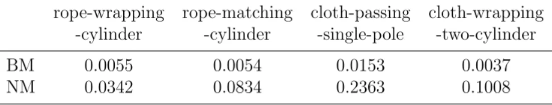
3.1 Top two rows: Mean computation time (ms) per model prediction for a given gripper motion. BT: Bullet simulator; CDR: constrained directional rigidity. Bottom row: Mean number of times the model was evaluated when executing the controller in Section 4.4. . . 24 4.1 Mean computation time (s) to compute the gripper motion for a given

state. BM: stretching avoidance controller; NM: stretching constraint controller. . . 39 5.1 Controller parameters . . . 48 5.2 KF-MANB and KF-MANDB parameters . . . 48 5.3 Synthetic trial results showing total regret with standard deviation

in brackets for all bandit algorithms for 100 runs of each setup. . . . 49 6.1 Deadlock prediction parameters . . . 83 6.2 Distance and planner parameters . . . 84 6.3 Planning statistics for the first plan for each example task in

sim-ulation, averaged across 100 trials. Standard deviation is shown in brackets. . . 90 6.4 Smoothing statistics for the first plan for each example task in

sim-ulation, averaged across 100 trials. Standard deviation is shown in brackets. . . 90 6.5 Local controller and deadlock prediction avg. computation time per

iteration for each type of deformable object, averaged across all trials. 91 6.6 Average computation time to compute the effect of a gripper motion. 91 6.7 Planning statistics for the cloth placemat example, averaged across

100 trials. Standard deviation is shown in brackets. . . 94 6.8 Smoothing statistics for the cloth placemat example, averaged across

100 trials. Standard deviation is shown in brackets. . . 94 7.1 Planning statistics, averaged over 30 trials . . . 114

(13)

ABSTRACT

This dissertation is motivated by two research questions: (1) How can robots perform a broad range of useful tasks with deformable objects without a time con-suming modelling or data collection phase? and (2) How can robots take advantage of information learned while manipulating deformable objects?

To address the first question, I propose a framework for deformable object manip-ulation that interleaves planning and control, enabling complex manipmanip-ulation tasks without relying on high-fidelity modeling or simulation. Each part of the framework uses a different representation of the deformable object that is well suited for the specific requirements of each component. The key idea behind these techniques is that we do not need to explicitly model and control every part of the deformable object, instead relying on the object’s natural compliance in many situations.

For the second question, I consider the two major components of my framework and examine what can cause failure in each. The goal then is to learn from experience gathered while performing tasks in order to avoid making the same mistake again and again. To this end I formulate the controller’s task as a Multi-Armed Bandit problem, enabling the controller to choose models based on the current circumstances. For the planner, I present a method to learn when we can rely on the robot’s model of the deformable object, enabling the planner to avoid generating plans that are infeasible. This framework is demonstrated in simulation with free floating grippers as well as on a 16 DoF physical robot, where reachability and dual-arm constraints make the tasks more difficult.

(14)

CHAPTER I

Introduction

In the 1950s and 1960s George Devol, Joseph Engleberger, and many others be-gan developing machines that were programmable manipulators of objects. Indus-trial manufacturers, in a desire to reduce labour costs, improve quality, and reduce delivery times were early adopters of this technology. These industrial robots were programmed to perform highly repetitive manipulation of various rigid objects in fixed environments. Key to the robot’s success are the specific program instructions derived from previously measured and calculated features of the real-world objects under manipulation in a fixed environment. The pervasive use of industrial robots performing flawlessly around the globe in factories performing tasks like medical lab-oratory testing, automobile assembling, or electronics circuit board manufacturing demonstrate the success of programmable manipulators of objects. Complexity has increased, dexterity has improved, and a given robot may be capable of more than one task or can be applied to a different, but previously known size of object or in a different, fully described environment; but, the vast majority of the modeling and planning remains a human creation and is merely programmed into the robot in advance. The industrial robot certainly does not learn.

Indeed, 35 years ago, Michael Brady [2] argued that “Since robotics is the field concerned with the connection of perception to action, Artificial Intelligence must have a central role in Robotics if the connection is to be intelligent.” Since then, there have been great strides made developing robots with intelligence; one promi-nent example of this is the self-driving automobile. Like industrial manipulators, a self-driving automobile knows much about its own dimensions and physics but it is constantly relying on computation-intensive processes for intelligence. The robot’s task is achievable because the environment being modeled is rigid, the automobile’s dynamics are known, and advancements in computing speed have soared, making it possible for the robot to execute a very large, but finite, number of calculations

(15)

quickly enough for secure and accurate control. Brady went on to say, “Robotics challenges AI by forcing it to deal with real objects in the real world.” As true as that statement certainly is for robots such as self-driving automobiles, it is all the more true for robots that manipulate deformable objects possessing an infinite num-ber of degrees of freedom and the inherently incomplete description of the object in all of its possible arrangements. An interesting example of a robot that manipulates deformable objects in current use is the da Vinci surgical robot, well known for its YouTube video demonstrating it stitching a grape back together with thread. Its relevance to this paper is simple: The surgical robot does not learn, plan, or control anything directly; those computationally intensive tasks are performed by a human who controls the robot’s manipulating tools. The only way an argument could be made for declaring this surgical robot a learning, autonomous robot would be to as-sume that it ships from the factory, complete with a human operator who is deemed one of its components. Computational intensity is one of it’s biggest hurdles. The computational challenge posed by modeling, planning, and control for deformable objects will be addressed in this dissertation; and, we describe a framework that we successfully used to obtain measurable improvements against that challenge.

Traditional motion planning techniques such as A*, probabilistic roadmaps, and rapidly-exploring random trees were designed with rigid body motion in mind. In this framework contact with the environment is explicitly disallowed. In order to manipulate an object a typical approach is to build a model of the object being grasped; this model is then used to ensure that the object does not collide with anything during a particular motion. In contrast, when working with deformable objects, interaction with the environment is common (and often required), with the deformable object complying to the environment rather than colliding with it. This raises the question “How accurate do our models need to be?” There are a broad range of deformable object manipulation tasks that robots have performed without highly accurate models ranging from surgical applications [3] to knot-tying [4]. While these methods have some success they rely on either a hand designed sequence of actions (or controllers), or a time-consuming data collection phase.

To address these limitations, this dissertation is motivated by two key research questions: (1) How can robots perform a broad range of tasks with deformable objects without high-fidelity models and simulation? and (2) How can robots take advantage of information learned while manipulating deformable objects? By answering these questions we can take a step towards a household robot that is capable of performing a broad range of tasks without any additional training, and can improve its ability

(16)

to perform the specific tasks that it commonly encounters.

Examples of deformable object manipulation range from domestic tasks like fold-ing clothes to time and safety critical tasks such as robotic surgery. One of the challenges in planning for deformable object manipulation is the high number of de-grees of freedom involved; even approximating the configuration of a piece of cloth in 3D with a 4 × 4 grid results in a 48 degree of freedom configuration space. In addition, the dynamics of the deformable object are difficult to model [5]; even with high-fidelity modeling and simulation, planning for an individual task can take hours [6]. Local controllers on the other hand are able to very efficiently generate motion, however, they are only able to successfully complete a task when the initial configura-tion is in the “attracconfigura-tion basin” of the goal [7, 8]. We propose combining the strengths of global planning with the strengths of local control while mitigating the weakness of each; we propose a framework for interleaving planning and control which uses global planning to generate gross motion of the deformable object, and a local controller to refine the configuration of the deformable object within the local neighborhood. By separating planning from control we are able to use different representations of the deformable object, each suited to efficient computation for their respective roles.

Two key ideas allow this framework to reliably perform tasks without a time-consuming modelling or data collection phase. First, we do not need to explicitly model and control every part of the deformable object, instead relying on the object’s natural compliance in many situations. By doing so we drastically reduce the need for model fidelity, enabling the use of model approximations that do not need to be highly accurate. Second, our framework does not assume that the local controller or global planner are infallible. Instead, we assume that mistakes will be made, and implement learning algorithms designed to avoid making the same mistake again. To this end I formulate the controller’s task as a Multi-Armed Bandit problem, enabling the controller to chose models based on the current circumstances. For planning we present a planning formulation that explicitly exposes the challenge of planning with model approximations, as well as a method for learning when we can and cannot rely on a model approximation during planning.

This dissertation makes seven contributions towards answering these research questions:

• We introduce a more accurate geometric model of how the direction of gripper motion and obstacles affect deformable objects.

(17)

being overstretched by the robot as part of a local controller, allowing for the use of less accurate models without risking tearing the deformable object. • We formulate the task of the local controller as a Multi-Armed Bandit problem,

with each arm representing a model of the deformable object.

• We introduce a manipulation framework that interleaves planning and control, choosing each when most useful.

• We present a global motion planner to generate gross motion of the deformable object, and provide a proof of probabilistic completeness for our planner, which is valid despite the fact that our system is underactuated and we do not have a steering function.

• We introduce a novel formulation of planning in reduced state spaces.

• We propose a method for improving the performance of the global planner as mistakes are made due to model approximations, enabling the planner to learn from experience.

(18)

CHAPTER II

Related Work

Robotic manipulation of deformable objects has been studied in many contexts ranging from surgery to industrial manipulation (see [9, 10, 11] for surveys). Below we discuss the most relevant methods to the work presented in this dissertation, starting with methods of modelling and simulating deformable objects. We then discuss visual servoing and other local control methods for performing deformable object manipulation tasks. Next we discuss related work for model selection and using multiple models for control. We then describe work relevant to combining local controllers and global planners for accomplishing tasks. We conclude with related work in motion planning for deformable objects and ways to consider topology in planning.

2.1 Modelling Deformable Objects

Much work in deformable object manipulation relies on simulating an accurate model of the object being manipulated. Motivated by applications in computer graphics and surgical training, many methods have been developed for simulating string-like objects [12, 13] and cloth-like objects [14, 15]. The most common simu-lation methods use Mass-Spring models [16, 5], which are generally not accurate for large deformations [17], and Finite-Element (FEM) models [18, 19, 20]. FEM-based methods are widely used and physically well-founded, but they can be unstable when subject to contact constraints, which are especially important in this work. They also require significant tuning and are very sensitive to the discretization of the object. Furthermore, such models require knowledge of the physical properties of the object, such as it’s Young’s modulus and friction parameters, which we do not assume are known.

(19)

Also, we seek a model that can be evaluated very quickly inside an optimal con-trol framework, and Finite-element models, while accurate, can be computationally-expensive to simulate. While methods have been developed to track objects using FEM in real-time [21], a controller may need to evaluate the model many times to find an appropriate command, requiring speeds faster than real-time. Specialized models have also been developed, e.g., [22] and [23] focus on elastic rods that are not in contact. We seek a model that works well with rope-like and cloth-like materials that can deform as a result of contact. Finally, researchers have also investigated automatic modeling of deformable objects [24, 25]. However, these methods rely on a time-consuming training phase for each object to be modeled, which we would like to avoid.

Our work is complementary to methods that adapt the model of the object during manipulation [26, 27, 28]. Our model can serve as an initial guess and a reference for such methods so that the online adaptation process does not diverge too far from a reasonable model as a result of perception or modeling error. Our modelling methods build on the idea of diminishing rigidity Jacobians [7] by improving the model by considering the effects of the direction of motion and static obstacles that the deformable object interacts with.

2.2 Local Control for Manipulation Tasks

Given a model such as those above, researchers have investigated various control methods to manipulate deformable objects. Model-based visual servoing approaches bypass planning entirely, and instead use a local controller to determine how to move the robot end-effector for a given task [29, 30, 31]. Other approaches [7, 26, 32, 27] bypass the need for an explicit deformable object model, instead using approximations of the Jacobian to drive the deformable object to the attractor of the starting state. More recent work by Hu et al. [28] has enabled the use of Gaussian process regression while controlling a deformable object. Our work builds on Berenson [7], capturing overstretching and obstacle avoidance into control constraints that are more effective at preventing damage to the deformable object.

2.3 Using Multiple Models

In order to accomplish a given manipulation task, we need to determine which type of model to use at the current time to compute the next velocity command, as

(20)

well as how to set the model parameters. Frequently this selection is done manually, however, there are methods designed to make these determinations automatically. Machine learning techniques such as [33, 34] rely on supervised training data in order to intelligently search for the best regression or classification model. These methods are able to estimate the accuracy of each model as training data is processed, pruning models from the training that are unlikely to converge or otherwise outperform models that are kept. These methods are designed for large datasets rather than an online setting where we may not have any training dataa priori. While it may be possible to adjust these methods to consider model utility instead of model accuracy, it is unclear how to acquire the needed training data for the task at hand without having already performed the task. The most directly applicable methods come from the Multi-Armed Bandit (MAB) literature [35, 36, 37]. In this framework there are multiple actions we can take, each of which provides us with some reward according to an unknown probability distribution. The problem then is to determine which action to take (which arm to pull) at each time step in order to maximize reward.

The MAB approach is well-studied for problems where the reward distributions are stationary; i.e. the distributions do not change over time [36, 38]. This is not the case for deformable object manipulation; consider the situation where the object is far away from the goal versus the object being at the goal. In the first case there is a possibility of an action moving the object closer to the goal and thus achieving a positive reward; however, in the second case any motion would, at best, give zero reward. In the contextual bandits [39, 40] variation of the MAB problem, additional contextual information or features are observed at each timestep, which can be used to determine which arm to pull. Typical solutions map the current features to estimates of the expected reward for each arm using regressions techniques or other metric-space analysis. In order to use contextual bandits for a given task a set of features would need to be engineered, however it is not clear what features to use.

Recent work [41] on non-stationary MAB problems offer promising results that utilize independent Kalman filters as the basis for the estimation of a non-stationary reward distribution for each arm. This algorithm (KF-MANB) provides a Bayesian estimate of the reward distribution at each timestep, assuming that the reward is normally distributed. KF-MANB then performs Thompson sampling [38] to select which arm to pull, choosing each in proportion to the belief that it is the optimal arm. We build on this approach in this paper to produce a method that also accounts for dependencies between arms by approximating the coupling between arms at each timestep.

(21)

For the tasks we address, the reward distributions are both non-stationary as well as dependent. Because all arms are operating on the same physical system, pulling one arm both gives us information about the distributions over other arms, as well as changing the future reward distributions of all arms. While work has been done on dependent bandits [42, 39], we are not aware of any work addressing the com-bination of non-stationary and dependent bandits using a regret-based formulation. Our method for model selection is inspired by KF-MANB, however we directly use coupling between models in order to form a joint reward distribution over all models. This enables a pull of a single arm to provide information about all arms, and thus we spend less time exploring the model space and more time exploiting useful models to perform the manipulation task.

2.4 Motion Planning for Deformable Objects

Motion planning for manipulation of deformable objects is an active area of re-search [10]. Saha et al. [43] present a Probabilistic Roadmap (PRM) [44] that plans for knot-tying tasks with rope. Rodriguez and Amato [45] study motion planning in fully deformable simulation environments. Their method, based on Rapidly-exploring Random Trees (RRTs) [46], applies forces directly to an object to move it through narrow spaces while using the simulator to compute the resulting deformations. Frank et al. [47] presented a method that pre-computes deformation simulations in a given environment to enable fast multi-query planning. Other sampling-based approaches have also been proposed [48, 49, 50, 51, 52, 53]. However, all the above methods either disallow contact with the environment or rely on potentially time-consuming physical simulation of the deformable object, which is often very sensitive to phys-ical and computational parameters that may be difficult to determine. In contrast our method uses simplified models for control and motion planning with far lower computational cost.

Our planning method has some similarity to topological [54, 55] and tethered robot [56, 57] planning techniques; these methods use the topological structure of the space to define homotopy classes, either as a direct planning goal, or as a way to help inform planning in the case of tethered robots. Planning for some deformable objects, in particular rope or string, can be viewed as an extension of the tethered robot case where the base of the tether can move. This extension, however, requires a very different approach to homotopy than is commonly used, particularly when working in three-dimensional space instead of a planar environment. In our work we usevisiblity

(22)

deformations from [54] as a way to encode homotopy-like classes of configurations. Previous approaches to proving probabilistic completeness for efficient planning of underactuated systems rely on the existence of a steering function to move the system from one region of the state space to another, or choosing controls at random [58, 59, 60, 1]. For deformable objects, a computationally-efficient steering function is not available, and using random controls can lead to prohibitively long planning times. Roussel et al. [53] bypass this challenge by analyzing completeness in the submanifold of quasi-static contact-free configurations of a extensible elastic rods. In contrast, we show that our method is probabilistically complete even when contact between the deformable object and obstacles is considered along the path. Note that it is especially important to allow contact at the goal configuration of the object to achieve coverage tasks. Li et al. [1] present an efficient asymptotically-optimal planner which does not need a steering function, however, they do rely on the existence of a contact free trajectory where every point in the trajectory is in the interior of the valid configuration space. Our proof of probabilistic completeness is based on Li et al. [1], but we allow for the deformable object to be in contact with obstacles along a given trajectory.

2.5 Interleaving Planning and Control for Deformable

Ob-ject Manipulation

The use of a local controller is not considered in the above methods, instead relying on a global planner (and thus implicitly the accuracy of the simulator) to generate a path that completes the entire task. In contrast, our framework combines the strengths of global planning with the strengths of local control in order to perform tasks.

Park et al. [61] considered interleaving planning and control for arm reaching tasks in rigid unknown environments. In their method, they assume an initially unknown environment in which they plan a path to a specific end-effector position. This path is then followed by a local controller until the task is complete, or the local controller gets stuck. If the local controller gets stuck, then a new path is planned and the cycle repeats. In contrast, our controller is performing the task directly rather than following a planned reference trajectory, incorporating deadlock prediction into the execution loop, while our global planner is planning for both the robot motion as well as the deformable object stretching constraint.

(23)

object modelling challenges entirely by using offline demonstrations to teach the robot specific manipulation tasks [4, 62]; however, when a new task is attempted a new training set needs to be generated. In our application we are interested in a way to manipulate a deformable object without a high-fidelity model or training set available

a priori. For instance, imagine a robot encountering a new piece of clothing for a new task. While it may have models for previously-seen clothes or training sets for previous tasks, there is no guarantee that those models or training sets are appropriate for the new task.

2.6 Learning for Planning in Reduced State Spaces

In terms of applying machine learning to control and planning, prior work has primarily used learned dynamics models for control [63, 64, 65, 66, 67]. Recent work [68] has also explored planning in a learned reduced space, but they do not consider the error in a reduced model’s prediction when planning. Visual Planning and Acting (VPA) [69] learns a latent transition model based on visual input for planning. This work uses on a classifier to prune infeasible transitions during planning. However, despite this classifier, only 15% of generated plans were visually plausible, with only 20% of the visually plausible plans being executable. When considering machine learning methods in this dissertation we do not focus on learning a reduction but rather on creating a framework that can be used to overcome limitations in a given model reduction.

(24)

CHAPTER III

Deformable Object Modelling

One of the key challenges in manipulating deformable objects is the inherent difficulty of modeling and simulating them. While there has been some progress towards online modeling of deformable objects [24, 25] these methods rely on a time-consuming training phase for each object to be modeled. This training phase typically consists of probing the deformable object with test forces in various configurations, and then fitting model parameters to the generated data. While this process can generate useful models, the time it takes to generate a model for each task can be prohibitive for some applications. Of particular interest are Jacobian-based models; in these models we assume that there is some function F : SE(3)G _→

RN which

maps a configuration of G robot grippers q ∈ SE(3)G _{to a parameterization of the}

deformable object P ∈_RN_{, where} _N _{is the dimensionality of the parameterization of}

the deformable object. These models are then linearized by calculating the Jacobian of F: P =F(q) ∂P ∂t = ∂F(q) ∂q ∂q ∂t ˙ P =J(q) ˙q . (3.1)

Computation of an exact Jacobian J(q) at a given configuration q is often compu-tationally intractable and requires high-fidelity models anbd simulators, so instead approximations are frequently used.

In this chapter we discuss a diminishing-rigidity based approximation first intro-duced by Berenson [7] and extensions of this model. The diminishing-rigidity model assumes that points on the deformable object that are near a gripper move “almost rigidly” with respect to the gripper while points that are further away move “less

(25)

rigidly”. In addition to this Jacobian-based model, we also introduce a non-linear modification of the diminishing-rigidity Jacobian which more accurately captures the effect of the direction of gripper motion and obstacles.

3.1 Definitions

Let the robot be represented by a set ofGgrippers with configurationq∈SE(3)G_.

We assume that the robot configuration can be measured exactly; in this work we assume the robot to be a set of free floating grippers; in practice we can track the motion of these with inverse kinematics on robot arms (see Sec 4.3.2.2 for an imple-mentation). We use the Lie algebra [70] ofSE(3) to represent robot gripper velocities. This is the tangent space of SE(3), denoted as se(3). The velocity of a single gripper g is then ˙qg =

h

v_gT ω_gT

iT

∈se(3) wherevg andωg are the translational and rotational

components of the gripper velocity. We define the velocity of the entire robot to be ˙

q = hq˙T₁ . . . q˙T_G

iT

∈ se(3)G. We define the inner product of two gripper velocities ˙

q1,q2˙ ∈se(3) to be

hq1,˙ q2˙ i=vTv2+cωT₁ω2 , (3.2) where c > 0 is scaling factor relating rotational and translational velocities. This defines the se(3) norm

kq˙gk2se(3) =hq˙g,q˙gi . (3.3)

Let the configuration of a deformable object be a set ofP points with configuration P =hpT

1 . . . pTP

iT

∈_R3P_{. We assume that we have a method of sensing}_P_{. Let} _D

be a symmetricP ×P matrix whereDij is the the geodesic distance (see Figure 3.1)

between pi and pj when the deformable object is in its “natural” or “relaxed” state.

To measure the norm of a deformable object velocity ˙P =

h ˙ pT 1 . . . p˙TP iT ∈_R3P _we

will use a weighted Euclidean seminorm kPk˙ 2 W = P X i=1 wip˙iTp˙i = ˙PT diag (W) ˙P (3.4) where W = hw1 . . . wP iT

∈ _RP _{is a set of non-negative weights. The rest of the}

environment is denoted O and is assumed to be both static, and known exactly. The current state of the deformable object is a function of the current gripper pose P, the history of gripper motions that have been applied Qhist_{, the object’s initial}

(26)

Figure 3.1: Euclidean distance measures length of the shortest path betweenpi andpj

in_R3 _{(gold). Geodesic distance measures the length of the shortest path, constrained} to stay within the deformable object (red).

configuration P0, and the obstacles in the environment O:

P =F(q, Qhist,P0,O) . (3.5) Let a deformation model φ be defined as a function which takes as input the system configuration, gripper velocities, and obstacle configuration to a deformable object and returns a deformable object velocity:

˙

P =φ(q,q,˙ P,O) . (3.6)

For brevity this will frequently be shortened to ˙P =φ( ˙q).

For Jacobian based models, we take the time derivative of Eq. (3.5) to get dP dt = ∂F ∂q ∂q ∂t + ∂F ∂Qhist ∂Qhist ∂t + ∂F ∂P0 ∂P0 ∂t + ∂F ∂O ∂O ∂t . (3.7)

Only the first term is non-zero, thus ˙

P = ∂F(q, Q hist_,_P

0,O)

∂q q˙=J(q,q,˙ P,O) ˙q. (3.8) Note that Qhist _and _P

0 are needed in F to compute the current state of the object, but if we can sense P directly (as we assume), then Qhist _and _P

0 are not needed to compute the Jacobian J. Thus for Jacobian based models Eq. (3.8) directly defines the deformation modelφ

(27)

3.2 Diminishing Rigidity Jacobian

The key assumption used by this method [7] is diminishing rigidity: the closer a gripper is to a particular part of the deformable object, the more that part of the object moves in the same way that the gripper does (i.e. more “rigidly”). The further away a given point on the object is, the less rigidly it behaves; the less it moves when the gripper moves. In this section we refine Berenson’s method by redefining J_i,grot and introducing an extra parameter. This results in two parameters ktrans ≥ 0 and krot _≥ _{0 which control how the translational and rotational rigidity scales with} distance. Small values entail very rigid objects such as steel cable; high values entail very deformable objects such as fine string.

For every pointiand every gripperg we construct a JacobianJrigid_{(i, g) such that} if pi was rigidly attached to the gripper qg then

˙

pi =Ji,grigidq˙g =

h

Jtrans

i,g Ji,grot

i

˙

qg . (3.10)

We then modify this Jacobian to account for the effects of diminishing rigidity. Let the indices of the set of points grasped by gripperg beGg ⊆ {1, . . . , P}. Letc(i, g) be

the index of the point with minimal relaxed geodesic distance to pi among the ones

grasped by gripper g:

c(i, g) = argmin

j∈Gg

Dij . (3.11)

Then the translational rigidity of point i with respect to gripperg is defined as w_i,gtrans =e−ktransDic(i,g) _(3.12) and the rotational rigidity is defined as

w_i,grot=e−krotDic(i,g)_. _(3.13) To construct an approximate Jacobian ˜J(i, g) for a single point and a single gripper we combine the rigid Jacobians with their respective rigidity values

˜

J(i, g) =hwtrans

i,g Ji,gtrans wroti,gJi,grot

i

(28)

and then combine the results into a single matrix ˜ J(q,P) =        ˜ J(1,1) J(1,˜ 2) . . . J(1, G)˜ ˜ J(2,1) . .. .. . ˜ J(P,1)        . (3.15)

3.3 Constrained Directional Rigidity

While the diminishing rigidity Jacobian method has been used to do practical manipulation tasks with a deformable object [7], we observe that this rigidity does not only diminish as the distance from the gripper increases. Instead, it is a function of a larger set of variables derived from the configuration of the object. First, the rigidity also depends on the direction of gripper motion. Figure 3.2 shows an example of an object’sdirectional rigidity. In addition capturing the effects of directional rigidity, in this section we seek to address contact with the environment, increasing the accuracy of the approximation.

Figure 3.2: An illustrative example of directional rigidity. Left: The rope moves almost rigidly when dragging it by one end to the left. Right: The rope deforms when pulling it on the right in the opposite direction.

3.3.1 Model Overview

In Section 3.2, J is assumed to be independent of ˙q and O, yielding ∂F ∂q =

J(q, Qhist_,_P

0) = J(q,P), which is analogous to a rigid-body Jacobian. While these assumptions allow a linear relationship between ˙q and ˙P, and thus computational convenience, they are not accurate in many situations (see Figure 3.2 for an exam-ple). In this section we augment the definition of J to include effects from ˙q and

(29)

O:

˙

P =J(q,q,˙ P,O) ˙q =φ(q,q,˙ P,O) . (3.16) We now describe how J is approximated, focusing on how it accounts for direc-tional rigidity (using ˙q) and how it enforces obstacle penetration constraints (using O).

3.3.2 Directional Rigidity

We build on the idea proposed by Berenson [7], which approximates J based on the observation that the deformable object behaves rigidly near points grasped by the robot grippers. [7] encoded this effect through a simple function that only considered the distance of a point from the the nearest gripper. However, we find that we can exploit geometric information in the object’s configuration to better predict the object’s motion when we use a more complex model. We have observed that the key features of the deformable object configuration for predicting its motion are its deformability (which is determined by its material properties) and where it is slack. The deformation influences the transmission of the force from the grippers, i.e., the more stretchable the object, the more it will stretch when force is applied. However, when a region of the object is taut, regardless of how stretchable it is, it will move as if it were rigidly connected to a gripper (e.g. imagine a rope held taut by two grippers). We also must take into account that points are not influenced equally by different grippers; i.e., grippers farther away contribute less to the motion of a point than those closer to it.

To incorporate the above effects into our model, we define the following variables, which can be derived from q,q, and˙ P:

• Dij: the geodesic distance (a scalar) between points pi and pj on the surface of

the object.

• vij: the vector starting at a point pi and ending at the point pj, as shown in

Figure 3.3.

• qg: the configuration of gripper g.

• q˙g: the velocity of gripper g.

Furthermore, let c(i, g) be the index of the point with the minimal geodesic dis-tance to pi among the ones grasped by the g’th gripper. We address the notion of

(30)

Figure 3.3: The length of the the red segment on the rope is the geodesic distance Dij. vij is the vector showing the relative position of pj with respect topi.

the rigidity as a function ofDic(i,g),vic(i,g), and ˙qg. For each point i and gripperg we

compute

˜

J(i, g) =θi,g

h

wtrans

i,g Ji,gtrans wroti,gJi,grot

i

w_i,gtrans =wtrans(Dic(i,g), vic(i,g),q˙g)

w_i,grot =wrot(Dic(i,g))

(3.17)

wtrans _and_wrot _{are the corresponding translational and rotational diminishing rigidity} factors defined by pi and gripper g (discussed below).

Our goal is to encode the directional rigidity of the object motion into wtrans and wrot and use θi,g to describe the influence of gripper g on pi. Intuitively, wtrans

should decrease with the increasing geodesic Dic(i,g) distance between pi and pc(i,g). This is because the deformation of the region betweenpi and pc(i,g) will attenuate the transmitted force of the gripper’s motion unless the object is taut. Since the effects onwrot

i,g from ˙qg and vic(i,g) are not as clear or significant as Dic(i,g), we keep wi,grot as a

function of Dic(i,g), where 1. wrot

i,g ranges between 0 and 1.

2. w_i,grot decreases as Dic(i,g) increases. We give the definition of w_i,grot below.

From observation, we find two key reasons related to the slackness of the object that induce the diminishing rigidity effect for translation motion, and we aim to encode these factors into wtrans

i,g . The first case is that the moving direction of ˙qg

makes the region on the object between pi and pc(i,g) less taut. The second case is that this region is already slack. wtrans

i,g is thus a product of two terms:

(31)

where αi,g addresses the effect in the first case (motion reducing tension), and βi,g

addresses the effect in the second case (object slackness). Both αi,g and βi,g are

functions of some of qg,q˙g, pi, or variables derived from these.

Forpion the object, we findαi,gis greatly impacted byvic(i,g)andvg. Decomposing

vg into vgrad, the component in the direction of vic(i,g), and vgperp, the component

perpendicular tovic(i,g). We observed that ifvgrad is in the opposite direction tovic(i,g), then it is more likely to make the intervening region slacker and thus reduce the transmission of force from the gripper to pi. Moreover, if vgrad and vic(i,g) are in the same direction when the object is not already slack, pi can move almost rigidly with

˙

qg. Figure 3.2 shows an example of the impact of this alignment. Based on these

observations, we design the functionαi,g =α(vic(i,g),q˙g) with the following properties:

1. α(vic(i,g),q˙g) ranges between 0 and 1.

2. α(vic(i,g),q˙g)> α(vjc(j,g),q˙g) if vic(i,g), vg >vjc(j,g), vg

and Dic(i,g) =Djc(i,g). 3. α(vic(i,g),q˙g)> α(vjc(j,g),q˙g) if vic(i,g), vg =vjc(j,g), vg

and Dic(i,g) > Djc(i,g). We give the definition of α(vic(i,g),q˙g) below.

As mentioned above, βi,g depends on the current slackness of the intervening

re-gion. Without other external forces applied on the object, the pulling force applied by the robot will tend to unwind or unfold the object eventually (we do not consider cases where the object is tied into knots). For this reason, the part of the interven-ing region on the object that is not already spread out is less likely to move rigidly with gripperg. One indicator that can address this property is the ratio between the Euclidean distance between pi and pc(i,g), and the geodesic distance Dic(i,g) between them. We denote ri,g =

||vic(i,g)||

Dic(i,g) to be this ratio. A larger ri,g indicates a tauter inter-vening region. A tauter interinter-vening region is more likely to result in ˙pi moving more

rigidly. Thus we can design the function βi,g =β(ri,g) with the following properties:

1. β(ri,g) ranges between 0 and 1.

2. β(ri,g) = 1 if ri,g = 1.

3. β(ri,g)> β(rj,g) ifri,g >rj,g

Finally, θi,g, which captures the influence of gripper g on pi should have the

fol-lowing property (wherek is the index of a different gripper on the robot): 1. θi,g ranges between 0 and 1.

(32)

2. θi,g < θi,k if Dic(i,g) > Dic(i,k). 3. PG

m=1θi,m = 1.

Through experimentation, we obtained good results with the following functions: α(vic(i,g),q˙g) = ek

dir_D_ic(i,g)(_cos

∠(vic(i,g),vg)−1) β(ri,g) = _kv ic(i,g)k Dic(i,g) kdist

wrot_i,g =e−krotDic(i,g) θi,g = xg PG m=0xm xm = min{Dic(i,1), . . . , Dic(i,G)} Dm (3.19)

where kdir_, _kdist_{, and} _krot _{are non-negative parameters. Specifically, a larger} _kdir indicates a greater impact on the diminishing in the rigidity from the motion reducing tension. A larger kdist indicates a greater impact on the diminishing in the rigidity from the slackness of the object in the current state. A larger krot indicates a faster decrease in rotational rigidity as the distance from pi to the gripper increases.

3.3.2.1 Obstacle Penetration Constraints

By combining the contributions of each individual gripper using the model devel-oped above, we get a prediction of a point’s movement from

˜ pi = h J(i,1) . . . J(i, G) i ˙ q =Ji(q,q,˙ P) ˙q (3.20)

However, at this stage, we haven’t taken into account the effect from the obstacles O. Thus the predicted ˜pi can move pi into an obstacle.

When the prediction of pi enters the obstacle, we project any penetration by the

predicted ˜pi into the tangent space of the obstacle surface (Figure 3.4). Letdi <kp˜ik

be the distance to collision in direction ˜pi from point pi; let λi = kpd˜iik; let ni be the unit surface normal of the obstacle in contact; and let Ni = (I3×3 −~ni~n+i ). Then to

account for obstacles we compute ˜ Ji(q,q,˙ P,O) =    (λi+ (1−λi)Ni)Ji(q,q,˙ P) if pi+ ˜pi in collision Ji(q,q,˙ P) otherwise (3.21)

(33)

𝑝_𝑖 ෨ሶ𝑝 = 𝐽_𝑖𝑑𝑟 _{𝑞, ሶ𝑞, 𝒫 ሶ𝑞} Φi 𝑞, ሶ𝑞, 𝒫, 𝒪 = ሶ𝑝i

Figure 3.4: Projection process for points that are predicted to be in collision after movement.

To generateJ for all the points and grippers we computeJi(q,q,˙ P) for eachpi. These

matrices are modified using penetration constraints to get Ji(q,q,˙ P,O). These

ma-trices are then stacked to obtain J(q,q,˙ P,O). Finally, we arrive at our approximate model: φ(q,q,˙ P,O) = J(q,q,˙ P,O) ˙q.

3.4 Results

Our goal for the constrained directional rigidity model is to improve the accuracy of the deformable object motion model (for use in the controller in Section 4.4), while maintaining reasonable computation speed. Our benchmark model is the diminishing rigidity model described in Section 3.2. To evaluate our method we perform exper-iments in simulation and on a physical robot. The simulator used is Bullet physics [71], however, we emphasize that our method has no knowledge of the simulation parameters or simulation methods used therein. The simulator is used as a “black-box,” mainly to stand in for a perception system and to allow us to do repeatable experiments. The physical robot consists of two KUKA iiwa 7DoF arms with Robotiq 3-finger hands.

We ran experiments with scenarios involving both cloth and rope. The parameters we used for the benchmark method (Section 3.2) are its default best value found in [7]: ktrans =krot = 10 for rope and ktrans = krot = 14 for cloth. The parameters for the new model (Section 3.3) are set as kdir = 4, kdist = 10, krot = 20 for the new model. All experiments were run on a i7-8700K 3.7 GHz CPU with 32 GB of RAM. A video showing the experiments can be found at https://www.youtube.com/watch? v=Y-wPsPdQVgg.

(34)

3.4.1 Simulation Environment Model Accuracy Results

We evaluated model accuracy by pulling the rope in a straight line along the di-rection of the rope, then turning the gripper and pulling back towards the rope as shown in Figure 3.2. As shown in Figure 3.5, our new model is a better approxima-tion of the true moapproxima-tion when the gripper is pulling the rope. When the gripper is turning, both the baseline and the new model produce comparable error, but when the gripper starts pulling again (this time in the opposite direction), the new model is a significantly better approximation.

We also evaluated model accuracy by pulling the cloth in a similar fashion; pulling the cloth one way, turning the grippers, and then pulling in the opposite direction. As shown in Figure 3.6, our new model is a better approximation of the true motion when the grippers are pulling the cloth. As in the rope test, when rotating the grippers both models produce comparable error. While the cloth is folded on itself both models produce noisy results, but when the cloth lies flat again, the new model achieves lower error.

Figure 3.5: RMS model prediction error for the simulated rope model accuracy test. The gripper pulls the rope for the first 4.5 seconds, then turns for half a second, then moves in the opposite direction at the 5 second mark.

(35)

Figure 3.6: RMS model prediction error for the simulated cloth model accuracy test. The grippers pull the cloth for the first 2.3 seconds, then turn for 0.63 seconds, then move in the opposite direction at the 2.93 second mark. At the 5 second mark the cloth is no longer folded.

3.4.2 Physical Robot Experiments

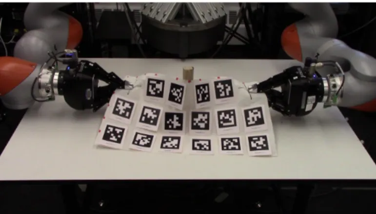
To evaluate our new model on a physical system, we set up an experiment with a cloth-like object manipulated by two 7DoF KUKA iiwa arms (Figure 3.7). To sense the position of the cloth, we use the AprilTags [72] and IAI Kinect2 [73] libraries. We use the same parameters as we used for simulated experiments. This test, which eval-uates model accuracy, uses a motion profile similar to the simulation accuracy tests (Figure 3.8). Similar to the simulation results, the new model improves performance when dragging the cloth (first and last sections of Figure 3.8), and is comparable during rotational motion and when the cloth is resting on edge perpendicular to the table (see video).

(36)

Figure 3.7: Initial setup for the physical robot model accuracy experiment.

Figure 3.8: RMS model prediction error for the physical cloth accuracy test. The grippers pull the cloth toward the robot for the first 10 timesteps, upward for 5 timesteps, rotate for 15 timesteps, diagonally down and away for 9 timesteps, then directly away from the robot.

(37)

3.4.3 Computation Time

To verify the practicality of our method, we gathered data comparing its com-putation time to the benchmark’s and to using the Bullet simulator for a variety of tasks (see Figure 3.9 and Section 4.5). Table 3.1 shows a comparison between the average time needed to evaluate the new model and the time needed to simulate a gripper motion with the Bullet simulator. Note that the amount of time required for the simulator to converge to a stable estimate depends on many conditions, includ-ing what object is beinclud-ing simulated. Through experimentation we determined that 4 simulation steps were adequate for rope and 10 for cloth. Comparing the time needed to do this simulation to the time needed to evaluate our model, we see that the new model is indeed faster by at least an order of magnitude, in some cases by two orders of magnitude, confirming that, despite being slower than the diminishing rigidity model, our method still outperforms the simulator in terms of computation time. This is particularly important given the average number of times a model is evaluated in a control loop.

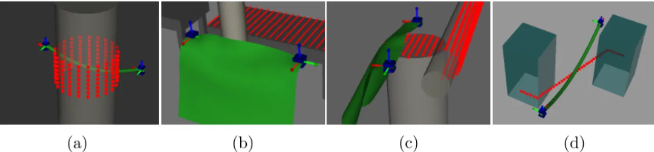
(a) (b) (c) (d)

Figure 3.9: Initial state of the four experiments, where the red points act as attractors for the deformable object. (a) Rope wrapping cylinder. (b) Cloth passing single pole. (c) Cloth covering two cylinders. (d) Rope matching zig-path

Table 3.1: Top two rows: Mean computation time (ms) per model prediction for a given gripper motion. BT: Bullet simulator; CDR: constrained directional rigidity. Bottom row: Mean number of times the model was evaluated when executing the controller in Section 4.4. rope-wrapping -cylinder rope-matching -cylinder cloth-passing -single-pole cloth-wrapping -two-cylinder BT 0.686 0.571 19.29 3.680 CDR 0.029 0.014 1.172 0.339 # evals 50.72 143.5 83.81 63.32

(38)

CHAPTER IV

Local Control

The previous chapter presented multiple models that approximate the effects of gripper motion on the deformable object. Next we introduce controllers that use these models as part of our framework for performing a broad range of tasks.

The role of the local controller is not to perform the whole task, but rather to refine the configuration of the deformable object locally. For our local controller we use a controller of the form introduced in [7] and [8]. These controllers locally minimize error while avoiding robot collision and excessive stretching of the deformable object. We present two different methods for addressing overstretch in sections 4.3 and 4.4. Both of these controllers rely on the same method for computing the direction to move the deformable object in order to reduce task error.

4.1 Problem Statement

We define a task based on a set ofT target pointsT ∈_R3T_{, a function}_ρ(T_,_P₎_≥_0,

which measures the alignment error between P and T, and a termination function Ω(T,P) which indicates if the task is finished. The methods we present in this chapter are local, i.e. at each time t they choose an incremental movement ˙qt which reduces

the alignment error as much as possible at time t+ 1: min

˙

qt

ρ(T,Pt+1) (4.1)

where Pt+1 is the result of executing ˙qt for one unit of time. ˙qt must also be feasible,

i.e. it should not bring the grippers into collision with obstacles and should not cause the object to stretch excessively.

(39)

4.2 Reducing Task Error

We build on previous work [7], splitting the desired deformable object movement into two parts: an error correction part and a stretching correction part. When defining the direction we want to move the deformable object to minimize error we calculate two values: which direction to move the deformable object points ˙Pe and

the importance of moving each deformable object point We. This is analogous to

computing the gradient of error, as well as an “importance factor” for each part of the gradient. We need these weights to be able to differentiate between points of the object where the error function is a plateau versus points where the error function is at a local minimum (Figure 4.1). Typically this is achieved using a Hessian, however our error function does not have a second derivative at many points.

Figure 4.1: Top Line: moving the point does not change the error, thus the desired movement is zero, however, it is not important to achieve zero movement, thus Wd=

0. Bottom Line: error is at a local minimum; thus moving the point increases error. In order to calculate ˙PeandWe, we start by defining a workspace navigation

func-tion for each target point Tk ∈ T towards Tk using Dijkstra’s algorithm. This gives

us the shortest collision-free path between any point in the workspace and the target point, as well as the distance travelled along that path. Using these distances, at ev-ery timestep for evev-ery target pointTk, we recalculate which point on the deformable

object pi is closest (Alg. 1). The directions each navigation function indicates are

added together to define the overall direction to manipulate a point (Alg. 2 line 5). For the importance factorsWe,i, we take only the largest distance thatpi would have

to move as a way to mitigate discretization effects (Alg. 2 line 6).

4.3 Stretching Avoidance Controller

An outline of how this controller functions is shown in Alg. 3; first, we calculate the error reduction direction and weight as discussed in the previous section (Lines 2 and 3). These error reduction terms are then combined with stretching avoidance terms ˙Ps, Ws to define the desired manipulation direction and importance weights

(40)

Algorithm 1 CalculateCorrespondences(P,T) 1: P_C = [∅]₁×P 2: for k ∈ {1,2, . . . , T} do 3: i←argmin_j∈{1,2,...,P}dDijkstras(Tk, pj) 4: d←dDijkstras(Tk, pi) 5: P_C[i]← {PC[i]∪(k, d)} 6: end for 7: return PC Algorithm 2 FollowNavigationFunction(P,PC) 1: P˙_e ←03P×1 2: We ←0P×1 3: for i∈ {1,2, . . . , P}do 4: for (k, d)∈ PC[i] do

5: p˙e,i ←p˙e,i+ DijkstrasNextStep(pi, k)

6: We,i ←max(We,i, d)

7: end for

8: end for

9: return P˙e, We

˙

Pd, Wd at each timestep (Lines 3 and 3). We then find the best robot motion to

achieve the desired deformable object motion, while preventing collision between the robot and obstacles (Line 5).

Algorithm 3 StretchingAvoidanceController(q,P,T) 1: P_C ← CalculateCorrespondences(P,T) 2: P˙e, We ← FollowNavigationFunction(P,PC) 3: P˙_s, Ws ← StretchingCorrection(P) 4: P˙_d, Wd← CombineTerms( ˙Pe, We,P˙s, Ws) 5: q˙cmd ← FindBestRobotMotion(q,P,P˙d, Wd) 4.3.1 Stretching Correction

Our algorithm for stretching correction is similar to that found in [7], with the addition of a weighting term ks, and a change in how we combine error correction

and stretching correction. We use the StretchingCorrection() function (Alg. 4) to compute ˙Ps and Ws based on a task-defined stretching threshold Ws ≥ 0. First we

compute the distance between every two points on the object and store the result in E. We then compare E to D which contains the relaxed lengths between every pair of points. If any two neighbouring points are stretched by more than a factor