Lehigh University
Lehigh Preserve
Theses and Dissertations
2017
Limited Memory Steepest Descent Methods for
Nonlinear Optimization
Wei Guo
Lehigh UniversityFollow this and additional works at:
http://preserve.lehigh.edu/etd
Part of the
Industrial Engineering Commons
This Dissertation is brought to you for free and open access by Lehigh Preserve. It has been accepted for inclusion in Theses and Dissertations by an authorized administrator of Lehigh Preserve. For more information, please [email protected].
Recommended Citation
Guo, Wei, "Limited Memory Steepest Descent Methods for Nonlinear Optimization" (2017).Theses and Dissertations. 2621. http://preserve.lehigh.edu/etd/2621
Limited Memory Steepest Descent Methods
for Nonlinear Optimization
by
Wei Guo
Presented to the Graduate and Research Committee of Lehigh University
in Candidacy for the Degree of Doctor of Philosophy
in
Industrial and Systems Engineering
Lehigh University May 2017
c
Copyright by Wei Guo 2017 All Rights Reserved
Approved and recommended for acceptance as a dissertation in partial fulfillment of the requirements for the degree of Doctor of Philosophy.
Date
Dr. Frank E. Curtis, Dissertation Director
Accepted Date
Committee Members:
Dr. Frank E. Curtis, Committee Chair Dr. Yu-Hong Dai
Dr. Daniel P. Robinson Dr. Katya Scheinberg Dr. Martin Tak´aˇc
Acknowledgements
I would like to thank first, and above all, my academic advisor, Professor Frank E. Curtis. It is my honor and privilege to have had him as my advisor. His extraodinary expertise, vision, and patience have guided me during my PhD study, especially his knowledgable insights on how to conduct meaningful and influential research, how to overcome various difficulties and challenges along the way, as well as how to work more efficiently and make good use of time. Besides his professional knowledge and thoughts, I have also received valuable suggestions on how to improve my technical writing skills and polish my commu-nication and presentation skills, which not only have benefitted me in the past years, but also will make my future career more successful and fruitful.
I also thank the remaining members of my dissertation committee — Professor Yu-Hong Dai, Professor Daniel P. Robinson, Professor Katya Scheinberg, and Professor Martin Tak´aˇc. Professor Yu-Hong Dai’s pioneering explorations and deep understanding in non-linear optimization have inspired the work in my dissertation a lot. Professor Daniel P. Robinson has made thoughtful suggestions and comments on our papers. Professor Katya Scheinberg has explained her knowledge and understanding in topics of optimization and machine learning through the courses she taught. Professor Martin Tak´aˇc has selflessly shared with me many of his helpful experiences and has given me guidance on research topic selections as well as presentation strategies. I also appreciate Professor Frank E. Curtis and Yu-Hong Dai for providing valuable suggestions and comments on my disser-tation.
I am also grateful to many people around me, including those warm-hearted aunts and uncles from the church and my close friends, who have played an important part of my
life and have helped me without hesitation when I am in need. Finally, most of all, I owe my deepest gratitude to my parents and grandparents. I could never have gone this far without their unconditional love, support, and encouragement.
Contents
Acknowledgements iv List of Tables x List of Figures xi Abstract 1 1 Introduction 32 Background and Literature Review 8
2.1 Convex Analysis . . . 9
2.1.1 Convexity . . . 9
2.1.2 Lipschitz Continuity . . . 9
2.1.3 Strong Convexity . . . 10
2.2 (Numerical) Linear Algebra . . . 10
2.2.1 Symmetric Positive Definite (SPD) Matrix . . . 10
2.2.2 Krylov Subspace and Krylov Sequence . . . 11
2.2.3 Rayleigh Quotient and (Harmonic) Ritz Value . . . 11
2.2.4 Lanczos Method . . . 13
2.2.5 QR Factorization . . . 14
2.2.6 Cholesky Factorization . . . 15
2.3 Basic Optimization Theory . . . 15
2.3.2 Optimality Condition . . . 17
2.3.3 Rates of Convergence . . . 18
2.3.4 Basic Iterations . . . 19
2.4 Steepest Descent Methods . . . 20
2.4.1 Introduction . . . 20
2.4.2 Krylov Sequence Generated from Steepest Descent Methods . . . 21
2.5 Barzilai-Borwein Methods . . . 22
2.6 Convergence Results . . . 23
2.7 Line Search Techniques . . . 24
2.7.1 Monotone Line Search . . . 24
2.7.2 Nonmonotone Line Search . . . 24
2.7.3 Summary . . . 26
2.8 Barzilai-Borwein Methods Variants . . . 27
2.8.1 Alternative Step (AS) Gradient Method . . . 27
2.8.2 Cyclic BB (CBB) Method . . . 28
2.8.3 Alternate Minimization (AM) Method . . . 29
2.8.4 Adaptive BB (ABB) Method . . . 30
2.8.5 Cubic Interpolation Model . . . 31
2.8.6 Modified Secant Equation Model . . . 32
2.8.7 Alternative Modified Secant Equation Model . . . 33
2.8.8 Other Stepsizes and Models . . . 33
2.9 Fletcher’s Limited Memory Steepest Descent (LMSD) Method . . . 34
2.10 Stochastic Gradient (SG) Methods . . . 36
2.10.1 Introduction . . . 36
2.10.2 Stochastic Gradient (SG) Methods . . . 37
3 R-Linear Convergence of Limited Memory Steepest Descent 39 3.1 Introduction . . . 39
3.2 Fundamentals . . . 42
3.2.2 Limited memory steepest descent (LMSD) method . . . 43
3.2.3 Finite Termination Property of LMSD . . . 46
3.3 R-Linear Convergence Rate of LMSD . . . 48
3.3.1 Known Convergence Properties of LMSD . . . 48
3.3.2 R-Linear Convergence Rate of LMSD for Arbitrary m∈[n] . . . 49
3.4 Numerical Demonstrations . . . 62
3.5 LMSD with Harmonic Ritz Values . . . 68
3.6 Conclusion . . . 70
4 Handling Nonpositive Curvature in a Limited Memory Steepest Descent Method 71 4.1 Introduction . . . 72
4.2 Literature Review . . . 75
4.2.1 Barzilai-Borwein Methods . . . 75
4.2.2 Fletcher’s limited memory steepest descent (LMSD) method . . . . 77
4.3 Algorithm Descriptions . . . 78
4.3.1 An algorithm that stores information from one previous iteration . . 78
4.3.2 An algorithm that stores information fromm≥1 previous iteration(s) 85 4.4 Implementation . . . 95
4.5 Numerical Experiments . . . 96
4.6 Conclusion . . . 105
5 A Limited Memory Stochastic Gradient Method 106 5.1 Introduction . . . 107
5.2 Barzilai-Borwein Stochastic Gradient (BBSG) Method . . . 109
5.2.1 Motivation . . . 109
5.2.2 Algorithm Description . . . 109
5.3 Limited Memory Stochastic Gradient (LMSG) Method . . . 111
5.3.1 Algorithm Description . . . 111
5.4 Numerical Experiments . . . 118 5.4.1 Implementation . . . 118 5.4.2 Numerical Results . . . 120 5.5 Conclusion . . . 122 6 Conclusion 124 Biography 132
List of Tables
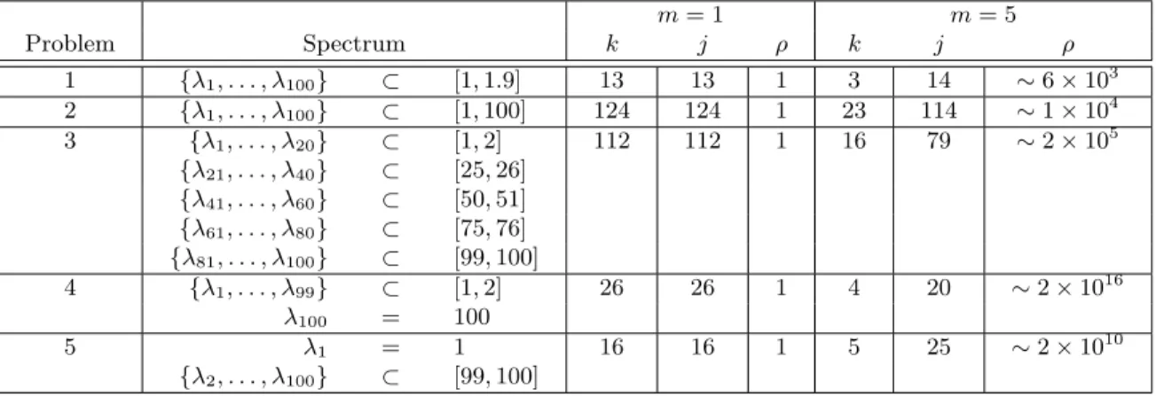
3.1 Spectra ofAfor five test problems along with outer and (total) inner itera-tion counts required by Algorithm LMSD and maximum value of the ratio
kR−1k k/(kgk,1k−1) observed during the run of Algorithm LMSD. For each
spectrum, a set of eigenvalues in an interval indicates that the eigenvalues
are evenly distributed within that interval. . . 63
4.1 Results form= 1 . . . 102
4.2 Results form= 3 . . . 103
4.3 Results form= 5 . . . 104
5.1 Dataset Description . . . 119
List of Figures
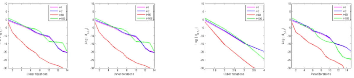
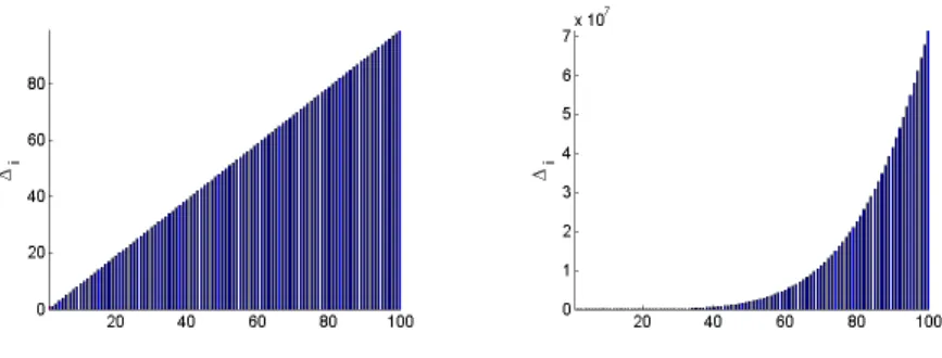
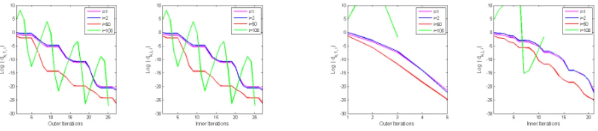
2.1 Global and local minima . . . 17 2.2 Stationary Point . . . 18 3.1 Weights in (3.10) for problem 1 with history lengthm= 1 (left two plots)
andm= 5 (right two plots). . . 65 3.2 Constants in (3.17) for problem 1 with history lengthm= 1 (left plot) and
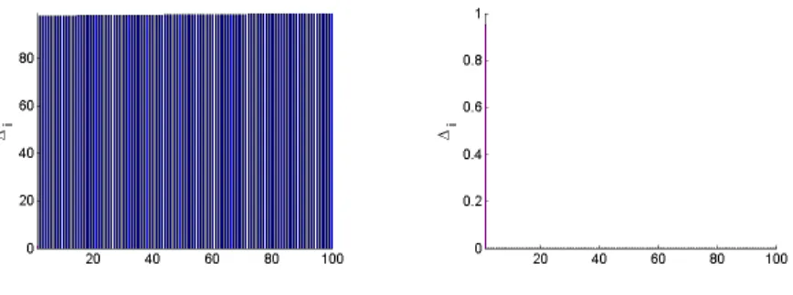
m= 5 (right plot). . . 65 3.3 Weights in (3.10) for problem 2 with history lengthm= 1 (left two plots)
andm= 5 (right two plots). . . 65 3.4 Constants in (3.17) for problem 2 with history lengthm= 1 (left plot) and
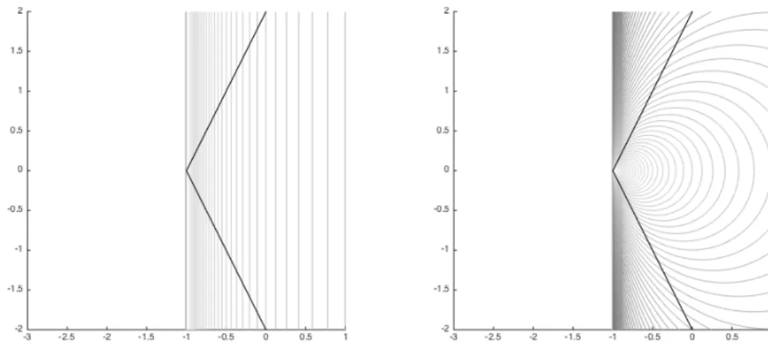
m= 5 (right plot). . . 66 3.5 Weights in (3.10) for problem 3 with history lengthm= 1 (left two plots)
andm= 5 (right two plots). . . 66 3.6 Constants in (3.17) for problem 3 with history lengthm= 1 (left plot) and
m= 5 (right plot). . . 66 3.7 Weights in (3.10) for problem 4 with history lengthm= 1 (left two plots)
andm= 5 (right two plots). . . 67 3.8 Constants in (3.17) for problem 4 with history lengthm= 1 (left plot) and
m= 5 (right plot). . . 67 3.9 Weights in (3.10) for problem 5 with history lengthm= 1 (left two plots)
3.10 Constants in (3.17) for problem 5 with history lengthm= 1 (left plot) and
m= 5 (right plot). . . 68
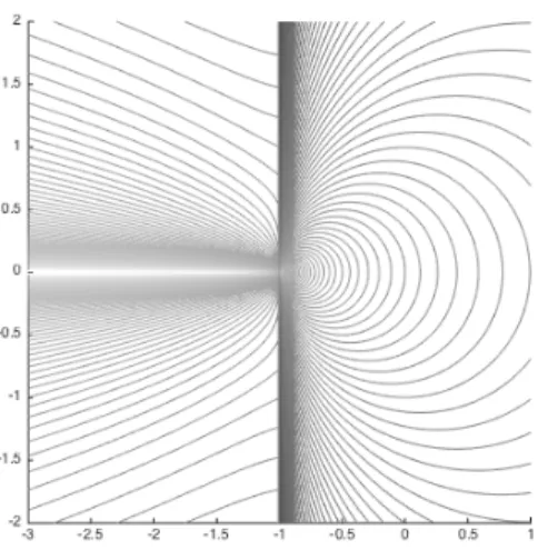
4.1 Illustration of the stepsizes computed, as a function of the gradientgk, in an algorithm in whichsTkyk >0 implies αk ←1/qk (left) versus one in which sTkyk >0 impliesαk ←1/qˆk (right). In both cases, sTkyk<0 implies αk is set to a constant; hence, no contour lines appear in the left half of each plot. 77 4.2 Illustration of the stepsizes computed, as a function of the current gradient gk, by Algorithm 5. . . 85
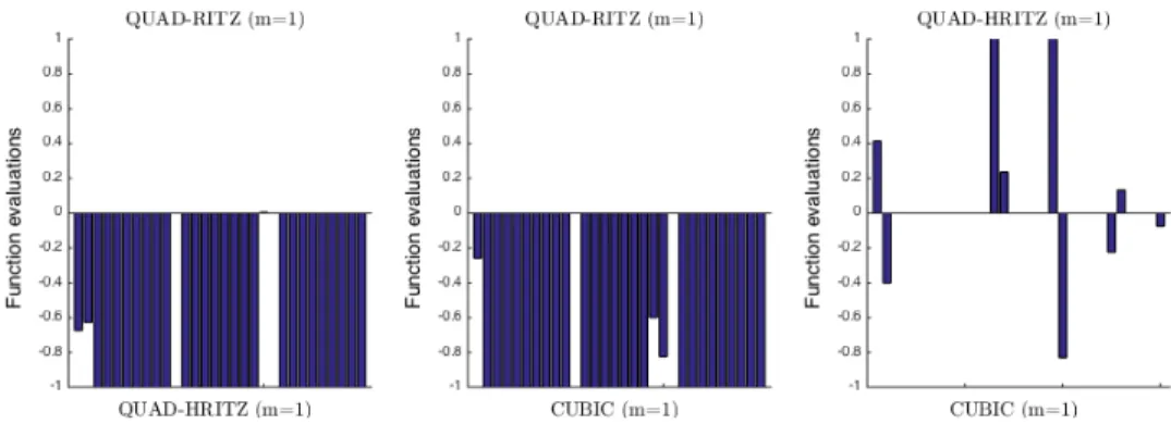
4.3 Outperforming factors for function evaluations withm= 1. . . 98
4.4 Outperforming factors for gradient evaluations withm= 1. . . 98
4.5 Outperforming factors for function evaluations withm= 3. . . 99
4.6 Outperforming factors for gradient evaluations withm= 3. . . 99
4.7 Outperforming factors for function evaluations withm= 5. . . 99
4.8 Outperforming factors for gradient evaluations withm= 5. . . 100
4.9 Outperforming factors for function evaluations forcubicform∈ {1,3,5}. . 100
4.10 Outperforming factors for gradient evaluations forcubicform∈ {1,3,5}. . 101
5.1 Stepsize and average function value for “a1a” (left two plots) and “aus-tralian” (right two plots). . . 121
5.2 Stepsize and average function value for “diabetes” (left two plots) and “ger-man.numer” (right two plots). . . 121
5.3 Stepsize and average function value for “heart” (left two plots) and “made-lon” (right two plots). . . 122
5.4 Stepsize and average function value for “splice” (left two plots) and “svmguide3” (right two plots). . . 122
Abstract
This dissertation concerns the development of limited memory steepest descent (LMSD) methods for solving unconstrained nonlinear optimization problems. In particular, we fo-cus on the class of LMSD methods recently proposed by Fletcher, which he has shown to be competitive with well-known quasi-Newton methods such as L-BFGS. However, in the design of such methods, much work remains to be done. First of all, Fletcher only showed a convergence result for LMSD methods when minimizing strongly convex quadratics, but no convergence rate result. In addition, his method mainly focused on minimizing strongly convex quadratics and general convex objectives, while when it comes to nonconvex ob-jectives, open questions remain about how to effectively deal with nonpositive curvature. Furthermore, Fletcher’s method relies on having access to exact gradients, which can be a limitation when computing exact gradients is too expensive. The focus of this dissertation is the design and analysis of algorithms intended to solve these issues.
In the first part of the new results in this dissertation, a convergence rate result for an LMSD method is proved. For context, we note that a basic LMSD method is an extension of the Barzilai-Borwein “two-point stepsize” strategy for steepest descent methods for solv-ing unconstrained optimization problems. It is known that the Barzilai-Borwein strategy yields a method with an R-linear rate of convergence when it is employed to minimize a strongly convex quadratic. Our contribution is to extend this analysis for LMSD, also for strongly convex quadratics. In particular, it is shown that, under reasonable assumptions, the method is R-linearly convergent for any choice of the history length parameter. The results of numerical experiments are also provided to illustrate behaviors of the method that are revealed through the theoretical analysis.
The second part proposes an LMSD method for solving unconstrained nonconvex opti-mization problems. As a steepest descent method, the step computation in each iteration only requires the evaluation of a gradient of the objective function and the calculation of a scalar stepsize. When employed to solve certain convex problems, our method reduces to a variant of LMSD method proposed by Fletcher, which means that, when the history length parameter is set to one, it reduces to a steepest descent method inspired by that proposed by Barzilai and Borwein. However, our method is novel in that we propose new algorithmic features for cases when nonpositive curvature is encountered. That is, our method is particularly suited for solving nonconvex problems. With a nonmonotone line search, we ensure global convergence for a variant of our method. We also illustrate with numerical experiments that our approach often yields superior performance when employed to solve nonconvex problems.
In the third part, we propose a limited memory stochastic gradient (LMSG) method for solving optimization problems arising in machine learning. As a start, we focus on prob-lems that are strongly convex. When the dataset is too large such that the computation of full gradients is too expensive, our method computes stepsizes and iterates based on (mini-batch) stochastic gradients. Although in stochastic gradient (SG) methods, a best-tuned fixed stepsize or diminishing stepsize is most widely used, it can be inefficient in practice. Our method adopts a cubic model and always guarantees a positive meaningful stepsize, even when nonpositive curvature is encountered (which can happen when using stochastic gradients, even when the problem is convex). Our approach is based on the LMSD method with cubic regularization proposed in the second part of this dissertation. With a projection of stepsizes, we ensure convergence to a neighborhood of the optimal solution when the interval is fixed and convergence to the optimal solution when the in-terval is diminishing. We also illustrate with numerical experiments that our approach can outperform an SG method with a fixed stepsize.
Chapter 1
Introduction
Mathematical optimization, where one models a real-world problem to minimize an ob-jective function over a set of variables that might need to satisfy certain constraints, has been a formal subject of research for decades and plays a significant role in many areas of engineering and applied mathematics. It arises in an abundant number of applications in multiple areas, including machine learning [7,48], control [32,30,51], compressed sensing [20, 9, 19], image processing [31,36], robust optimization [4], finance [25,37], optics [6], distance geometry [23], and many others. There are a variety of well-developed algorithm classes for solving optimization problems built, e.g., on steepest descent or (quasi-)Newton methodologies.
Optimization problems can be very large in size. In particular, one manner in which an optimization problem can be large is if it involves a large number of variables, say in the millions or more. For problems of such sizes, popular algorithms such as Newton’s method—a second-order method—might not be efficient for the following reasons.
• Second order derivatives (i.e., Hessian matrices) are expensive to compute.
• There may not be large enough space to store the Hessian matrices, even if they can be computed.
• They involve solving linear systems of equations, which can have high cost.
when solving large-scale optimization problems. Steepest descent methods have multiple advantages.
• Function and gradient evaluations are relatively cheap.
• It is beneficial to “move quickly” compared with Newton’s methods.
• Steepest descent methods are easily generalized for solving constrained problems (in that they are not complicated, e.g., by indefinite Hessian matrices).
Besides the advantages mentioned above, we can also combine (limited memory) quasi-Newton ideas with steepest descent methods to arrive at effective methods such as L-BFGS [40]. By applying these strategies, we do not only make computation during each iteration cheap but also save a lot of storage cost.
There are also other ways that an optimization problem can be large. For example, in machine learning, optimization problems arise when one wants to minimize an objective defined by a given dataset. There is the number of “samples” composing the dataset, and there is the number of optimization variables, which is often equal to the number of “features” contained in each sample. A challenge in “big data” problems is that either or both of the following can be true:
• The number of features can be very large.
• The number of samples can be very large.
In some situations, when not only the number of features, but also the number of samples is very large, the design of optimization method is complicated by the fact that the computation of a “full” gradient can be very expensive. When this is the case, stochastic gradient (SG) and its variants have been the main approaches for solving such problems. For example, stochastic gradient methods are actively used in machine learning, including support vector machine [52], linear and logistic regression [50], deep neural networks [1]— well known supervised learning models [39] for prediction and classfication.
The goal in this dissertation is to conduct research on limited memory steepest descent (LMSD) methods for solving nonlinear optimization problems. In particular, the class of
algorithms we explore is based on the work of Fletcher in [22], which in turn can be seen as an extension of the Barzilai-Borwein “two-point stepsize” strategy for steepest descent methods for solving unconstrained optimization problems [2].The extension can be quantified using a so-called history length parameter, for which we use the letterm. A BB method corresponds tom= 1, whereas LMSD involves any integerm∈[1, n].
For BB methods, there are now well-known properties when it is employed to minimize an n-dimensional strongly convex quadratic objective function. Such objective functions are interesting in their own right, but one can argue that such analyses also characterize the behavior of the method in the neighborhood of a strong local minimizer of any smooth objective function. In the original work (i.e., [2]), it is shown that the method converges
R-superlinearly when n = 2. In [44], it is shown that the method converges from any starting point for any natural numbern, and in [15] it is shown that the method converges
R-linearly for any suchn. In [22], it is shown that the proposed LMSD method converges from any starting point when it is employed to minimize a strongly convex quadratic.
However, to the best of our knowledge, the convergence rate of the method form >1 has not yet been analyzed. Our first contribution is to show that Fletcher’s LMSD method converges R-linearly when employed to minimize such a function. Our analysis builds upon the analyses in [22] and [15]. We also present the results of numerical experiments that illustrate our convergence theory and demonstrate that the practical performance of LMSD can be even better than the theory suggests.
Once the rate of convergence properties of LMSD method for strongly convex quadrat-ics are analyzed, in the second part, we focus on designing efficient algorithms within a steepest descent framework for solving general unconstrained optimization problems whose objective functions are continuously differentiable. The motivation of the work in this part is that, when it comes to solving nonconvex problems—which are not rare in practice— many methods falter and do not exhibit the same level of performance as when convex problems are considered. This also happens to the original BB method and LMSD method, which drives us to explore some alternative approaches for handling nonconvex problems. The main contribution of the new methodology we devise is that it provides a novel
strategy for computing stepsizes when solving nonconvex optimization problems. In par-ticular, when nonpositive curvature (as defined later) is encountered, our method adopts a local cubic model of the objective function in order to determine a stepsize (for m= 1) or sequence of stepsizes (for m ≥1). As in the case of the original BB methods and the LMSD method of Fletcher, our basic algorithm does not enforce sufficient decrease in the objective in every iteration. However, as is commonly done for variants of BB methods, we remark that, with a nonmonotone line search, a variant of our algorithm attains global convergence guarantees under weak assumptions. Our method also readily adopts the con-vergence rates attainable by a BB or LMSD method if/when it reaches a neighborhood of the solution in which the objective is strictly convex.
The motivation of the work in the third part is to solve the type of problems with not only a very large number of features but also a very large number of samples such that the computation of full gradients is very expensive. We focus on designing algorithms of the stochastic gradient (SG) variety. However, one of the major challenges in stochastic gra-dient (SG) methods is how to choose an appropriate stepsize while running the algorithm. Since traditional line search techniques are not readily applied in stochastic optimization methods, the common practice in SG is either to tune a stepsize by hand, or to tune a diminishing stepsize sequence, which can be time consuming and inefficient in practice.
Our contribution in this part is that we extend the BB (m= 1) and LMSD methods (m≥1) adopting cubic models using full gradient proposed in the second part to Barzilai-Borwein stochastic gradient method with cubic regularization (BBSG) and limited memory stochastic gradient method with cubic regularization (LMSG). We compute meaningful positive stepsizes from BBSG when m = 1 or LMSG when m ≥1 instead of using fixed or diminishing stepsizes. We also prove convergence (rate) properties for LMSG with fixed interval projection and diminishing interval projection for strongly convex objectives under mild assumptions, respectively. Furthermore, we conduct numerical experiments for LMSG on solving logistic regression problems. The numerical results show that LMSG can outperform SG with a fixed stepsize.
some mathematical bakground, including convex analysis, (numerical) linear algebra and basic optimization theory. We follow this by introducing literature on gradient-based methods (full gradient) for optimization, including steepest descent (SD) methods, BB methods and LMSD methods, their variants for computing stepsizes together with their theoretical properties. Next, we discuss stochastic gradient (SG) methods. Chapter 3
illustrates the R-linear convergence rate of LMSD for strongly convex quadratics, which extends the convergence rate analysis of BB methods. In Chapter 4, we propose an LMSD method for solving unconstrained optimization problems, especially when nonpos-itive curvature is encountered. In Chapter5, we design BBSG and LMSG methods within a stochastic gradient (SG) framework to solve “big data” problems. Final remarks and comments on all of the methods in this dissertation are presented in Chapter6.
Chapter 2
Background and Literature
Review
In this chapter, we first cover background on convex analysis, some fundamental (nu-merical) linear algebra and basic optimization theory. With this understanding of math-ematical background, we will introduce our first method, steepest descent (SD), which belongs to the class of gradient-based methods. This is followed by a literature review on Barzilai-Borwein (BB) methods, including algorithm descriptions and theoretical con-vergence results. Next, we will show how to incorporate line search techniques to BB methods as well as some BB methods variants. Followed by BB methods, we discuss lim-ited memory steepest descent (LMSD) methods, a generalization of BB methods. Finally, unlike all the methods mentioned above which apply full gradient during each iteration, we will explain in detail the methods that use a porportion of the full gradient, namely stochastic gradient (SG) methods.
We always assume matrixA(used in this chapter) is symmetric and thus all its eigen-values, λ1 ≤λ2≤ · · · ≤λn, are real.
2.1
Convex Analysis
In this Chapter, we provide some basic definitions and properties related to (strong) convexity and Lipschitz continuity.
2.1.1 Convexity
A real-valued functionf :Rn→R is convex if we have
f(αx+ (1−α)y)≤αf(x) + (1−α)f(y) for all (x, y)∈Rn×Rn andα∈[0,1]. (2.1) A functionf is strictly convex if forx6=yinequality (2.1) holds strictly. A convex function has the following properties.
• (Continuity) If f is convex, then it is continuous.
• (First order condition) If f is continuously differentiable, then we have
f(y)≥f(x) +∇f(x)T(y−x) for all (x, y)∈Rn×Rn. • (Monotone mapping) f is differentiable and convex if and only if
(∇f(x)− ∇f(y))T(x−y)≥0 for all (x, y)∈Rn×Rn.
2.1.2 Lipschitz Continuity
A function f :Rn→R is Lipschitz continuous if there exists a scalar L >0 such that
||f(x)−f(y)||2≤L||x−y||2 for all (x, y)∈Rn×Rn. (2.2)
Here are some properties related to Lipschitz continuity.
• f is convex if and only if L2xTx−f(x) is convex.
• (Quadratic upper bound) Suppose ∇f is Lipschitz continuous with parameter L, then convexity of g means that we can derive this upper bound forf:
f(y)≤f(x) +∇f(x)T(y−x) +L
2||y−x||
2
2 for all (x, y)∈Rn×Rn. (2.3)
2.1.3 Strong Convexity
A functionf :Rn→R is strongly convex with parameterσ >0 iff(x)−σ2xTxis convex.
A strongly convex function has the following properties.
• (First order condition)
f(y)≥f(x) +∇f(x)T(y−x) +σ
2||y−x||
2
2 for all (x, y)∈Rn×Rn. (2.4) • If f is strongly convex andx∗ is the unique minimizer, then
σ 2||x−x∗|| 2 2≤f(x)−f(x∗)≤ 1 2σ||∇f(x)|| 2 2 for all x∈Rn. (2.5)
2.2
(Numerical) Linear Algebra
2.2.1 Symmetric Positive Definite (SPD) Matrix
A symmetric matrix A ∈ Rn×n is positive definite (A 0) if and only if for all x ∈ Rn
and x6= 0, we have
xTAx >0.
Here are some basic properties of symmetric positive definite matrices.
• All A’s eigenvalues are real and positive.
0< λ1≤λ2 ≤ · · · ≤λn.
• A−1 exists and is also symmetric positive definite (A−1 0).
• The diagonal elements of matrix A are positive,aii>0.
• Eigenvalue decomposition.
There exists n×n orthogonal matrix U ∈ Rn×n, where UTU = U UT = I and
diagonal matrix Λ, such that
UTAU = Λ.
where Λ contains all eigenvalues of A.
• (Quadratic forms) A strongly convex quadratic functionf :Rn→ R can be
formu-lated asxTAxwherex is the column vector and Ais symmetric positive definite. 2.2.2 Krylov Subspace and Krylov Sequence
In linear algebra, the order m (m ≤ n) Krylov subspace generated by A ∈ Rn×n and a
vectorg∈Rnis the linear subspace spanned by the images of gunder the firstm powers
of A (starting fromA0 =I), that is,
Km(A, g) = span {g, Ag, A2g,· · · , Am−1g}.
And Aig, i= 0,1, · · · , m−1, the basis of Krylov subspace, are called Krylov sequence
initiated from g. More properties related to Krylov sequence will be discussed in steepest descent methods, i.e., Chapter2.4.2below.
2.2.3 Rayleigh Quotient and (Harmonic) Ritz Value For the m-dimensional Krylov subspace
starting from
q1= g ||g||,
we can generate orthonormal basis Q= {q1, q2, · · ·, qm} for Krylov subspace Km(A, g),
where Q∈Rn×m is orthogonal matrix and QTQ=I.
Sometimes the eigenvalues of matrixA∈Rn×ncan be expensive to compute especially
whennis very large, one basic idea is to formulate a smaller dimensional matrixT ∈Rm×m
and compute its m eigenvalues as approximations of the originalneigenvalues. A typical way is to project matrix A to them dimensional subspaceKm(A, g), i.e.
T =QTAQ,
and compute the m eigenvalues of matrixT.
When m = 1, Q =q1 ∈ Rn×1 with ||q1||22 = 1, the matrix T becomes a number, we
define this number as Rayleigh quotient R(A, q1), where R(A, q1) =q1TAq1.
The more general definition of Rayleigh quotient is
R(A, q1) = q
T
1Aq1 q1Tq1 .
with arbitrary q1∈Rn×1. In addition, the range of R(A, q1) is λ1≤R(A, q1)≤λn.
When we have general m ≥1 and obtain matrix T ∈Rm×m, we define m eigenvalues of
matrix T, i.e.
θm≤θm−1≤ · · · ≤θ1,
as Ritz values of matrix A, where
We also define meigenvalues of matrix (P−1T)−1, i.e.,
µm≤µm−1≤ · · · ≤µ1,
as harmonic Ritz values of matrix A, where
P =QTA2Q.
We haveT as a tridiagonal matrix and P as a pentadiagonal matrix when A is sym-metric. Here is the contrast of the computation of Ritz values and harmonic Ritz values. We write Θ =diag(θi), Ξ =diag(µi) and have the following eigensystems
(QTAQ)X= (QTQ)XΘ.
If we were to include an extraAin the innerproducts ofQTQandQTAQ, we would obtain a generalized eigensystem
(QTA2Q)X= (QTAQ)XΞ.
There are also alternative ways of computing matrices bothTandP whenAis unavailable, which will be explained in detail in Chapter 4.2.2.
Here is also a well known theorem revealing important interlacing relations between the eigenvalues of T, i.e. Ritz values and the eigenvalues of A. The theorem is known as the Cauchy Interlacing Theorem.
Theorem 2.2.1. The eigenvalues ofT (=QTAQ where QTQ=I) satisfy
θj ∈[λm+1−j, λn+1−j] for all j∈[m].
2.2.4 Lanczos Method
A well known method of computing matrixT from matrixAis the Lanczos method. Here is the algorithm framework.
Algorithm 1 Lanczos Method 1: input q1 ← ||gg||, q0 ←0, β1←0 2: for j= 1,2· · · , m−1do 3: wj0 ←Aqj 4: αj ←w0jqj 5: wj ←wj0 −αjqj−βjqj−1 6: βj+1← ||wj|| 7: qj+1← βj+1wj 8: end for 9: wm←Aqm 10: αm←w0mqm
From Lanczos method, we can getT ∈Rm×m, where
T = α1 β2 0 β2 α2 β3 β3 α3 . .. . .. . .. βm−1 βm−1 αm−1 βm 0 βm αm . 2.2.5 QR Factorization
Any real square matrix A∈Rn×n (not necessarily symmetric) may be decomposed as
A=QR,
whereQ is an orthogonal matrix (QTQ=I) andR is an upper triangular matrix. IfA is invertible, then the factorization is unique if we require that the diagonal elements of R
be positive.
More generally, we can factor an A ∈ Rn×m, with n ≥ m, as the product of an
(n−m) rows of an n×m upper triangular matrix consist entirely of zeros, it is often useful to partition R, or both R and Q:
A=QR=Q R1 0 = [Q1, Q2] R1 0 =Q1R1,
where R1 ∈ Rm×m is an upper triangular matrix, 0 ∈ R(n−m)×m is a zero matrix, Q1 ∈
Rn×m,Q2∈Rn×(n−m), andQ1 and Q2 both have orthogonal columns.
2.2.6 Cholesky Factorization
When A∈Rn×n is symmetric positive definite, we have
A=LLT,
where L∈Rn×n is a lower triangular matrix.
A closely related variant of the classical Cholesky decomposition is the LDL decom-position,
A=LDLT,
where L ∈ Rn×n is a lower triangular matrix and D ∈ Rn×n is a diagonal matrix. This
decomposition is related to the classical Cholesky decomposition, of the form LLT A=LDLT =LD12D 1 2TLT = (LD 1 2)(LD 1 2)T.
2.3
Basic Optimization Theory
Now that we have reviewed some knowledge of (numerical) linear algebra, we introduce some basic optimization theory focusing on unconstrained optimization. Consider the unconstrained optimization problem
min
x∈Rn
In this chapter, we discuss situations whenf :Rn→R is continuously differentiable (i.e.,
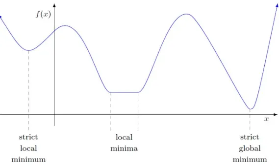
f ∈ C), or convex (with, perhaps,f /∈ C) and f is bounded below. 2.3.1 Global and Local Minima
Ideal minima are those that minimize a function globally over its domain.
Definition 2.3.1 (Global minimum). A vector x∗ is a global minimum of f if
f(x∗)≤f(x) for all x∈Rn.
Commonly, however, we are satisfied with a weaker form of minimum.
Definition 2.3.2 (Local minimum). A vector x∗ is a local minimum of f if there exists
>0 such that
f(x∗)≤f(x) for all x∈B(x∗, ) :={x∈Rn:kx−x∗k2 ≤}.
We also characterize certain types of global and/or local minima:
• x∗ is a strict global/local minimizer if the inequality holds strictly for x6=x∗.
• x∗ is an isolated global/local minimizer if, for some 0 > 0, it is the only local minimizer in the neighborhood B(x∗, 0).
An isolated minimum is a strict minimum, but (typically only for some pathological ex-amples) the reverse is not always true.
Figure 2.1: Global and local minima
A special fact in convex optimization is that all local minima are global minima.
Theorem 2.3.3. If f :Rn→Ris convex, then a local minimum off is a global minimum
of f. If f is strictly convex, then there exists at most one global minimum of f.
Unfortunately, for nonconvex optimization, the conditions in the definitions of global and local minima are not entirely useful, we rarely have global information about f, and so have no way to verify if a point is a global minimizer. Thus, in nonconvex optimization, we often focus on finding a local minimizer. Using calculus, we can derive local optimality conditions that aid in determining if a point is a local minimizer.
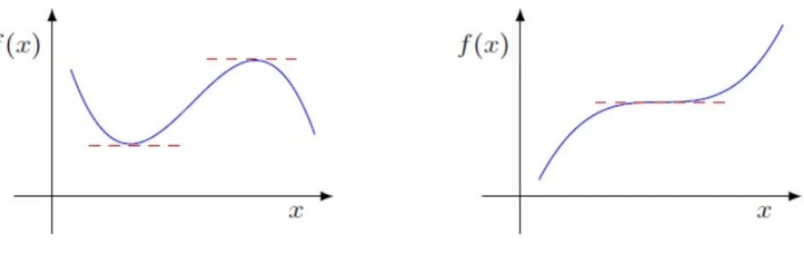
2.3.2 Optimality Condition
Theorem 2.3.4 (First-order necessary condition). If f ∈ C and x∗ is a local minimizer
of f, then ∇f(x∗) = 0.
We can limit our search to points where ∇f(x∗) = 0. However, ∇f(x∗) = 0 does not imply that we have a local minimizer.
Figure 2.2: Stationary Point
Definition 2.3.5 (Stationary point). A point x ∈ Rn is a stationary point for f ∈ C if
∇f(x) = 0.
2.3.3 Rates of Convergence
There are two types of rates of convergence of sequences, one prefixed byQ(for “quotient”) and the other prefixed by R (for “root”). Let{xk} ⊆Rn be a sequence that converges to
{x∗} ⊆Rn and let|| · ||be a vector norm on
Rn. There are different rates of convergence.
• The convergence of {xk} tox∗ isQ-sublinear if
lim
k→∞=
||xk+1−x∗|| ||xk−x∗|| = 1.
• The convergence of {xk} tox∗ isQ-linear if there existsc∈(0,1) such that
||xk+1−x∗|| ||xk−x∗||
≤c,
for all sufficiently large k. The constant cindicates the rate of linear convergence.
• The convergence of {xk} tox∗ isQ-superlinear if lim
k→∞=
||xk+1−x∗|| ||xk−x∗|| = 0.
It is easily seen that any sequence that converges Q-superlinearly also converges
We now distinguish between various types of Q-superlinear convergence.
• The convergence of {xk} tox∗ isQ-quadratic if there exists c >0 such that
||xk+1−x∗|| ||xk−x∗||2
≤c,
for all sufficiently large k.
• The Q-order of convergence of{xk} tox∗ isp >1 if there exists c >0 such that
||xk+1−x∗|| ||xk−x∗||p ≤c,
for all sufficiently large k. This leads to the definitions of Q-cubic (p = 3) and
Q-quartic (p= 4) convergence.
The above definitions only focus on the sequences decreasing monotonically, however, they do not cover the situation when certain sequences converge reasonably quickly but approach the limit point nonmonotonically. For such cases, we define a slightly weaker form of convergence known as R-order convergence. If{k}converges to 0 and
||xk−x∗|| ≤k for all k, (2.7)
then the R-order of convergence of {xk} to x∗ is said to be that of the Q-order of con-vergence of {k} to 0. If {k} converges Q-sublinearly to 0 and (2.7) holds, then {xk}
converges R-sublinearly to x∗; if {k} converges Q-linearly to 0 and (2.7) holds, {xk}
converges R-linearly tox∗; and so on. 2.3.4 Basic Iterations
Typically, we apply iterative methods for solving optimization problems, where the basic iterations have the form
In (2.8), xk is the current iteration point (at kth iteration), in order to reach the next
iteration point xk+1 (at (k+ 1)th iteration), we need two quantities: • Search direction dk, which direction to go.
• Stepsize αk, how far to go.
There are various ways of selecting each search direction and stepsize. For the choice of search direction, we mainly focus on negative gradient direction, where
dk=−gk. (2.9)
More will be discussed in Chapter 2.4. And for the computation of stepsize, we will introduce two well-known methods in Chapter2.5and2.9. For the purpose of guaranteeing algorithm convergence, sometimes a line search is also carried out to modify the original stepsize at each iteration, which will be explained in detail in Chapter 2.7.
We can also definesk+1:=αkdk as the step and thus
xk+1 =xk+sk+1, (2.10)
this notation is frequently used in Chapter 2.5.
2.4
Steepest Descent Methods
Following the discussion of some basic optimization theory, we will introduce one of the simplest and most widely used techniques for solving unconstrained nonlinear optimization problems, which is steepest descent (SD).
2.4.1 Introduction
First, let us consider unconstrained optimization problem 2.6. The simplest gradient-based method for solving this problem is a steepest descent method, which is the term we
use to describe any iterative method of the form
xk+1 ←xk−αkgk for all k∈N. (2.11)
Here, x0 ∈ Rn is a given initial point and, for all k ∈ N, the scalar αk > 0 is the kth
stepsize. In the classical steepest descent method of Cauchy, each stepsize is obtained by an exact line search (see [10]), i.e., assuming f is bounded below along the ray from xk
along −gk, one sets
αk ∈arg min
α≥0f(xk−αgk).
However, in modern variants of steepest descent, alternative stepsizes that are cheaper to compute are employed to reduce per-iteration (and typically overall) computational costs.
Algorithm 2 Steepest Descent Framework
1: input x0 ∈Rn 2: for k= 0,1,2· · · do 3: computegk← ∇f(xk) 4: choose αk∈(0,∞) 5: setxk+1←xk−αkgk 6: end for
2.4.2 Krylov Sequence Generated from Steepest Descent Methods Here is a property related to Krylov sequences. Given a strongly convex quadratic function with SPD matrix A, suppose we generate the consecutive iteration sequence
{xk−m, xk−m+1,· · ·, xk−1}by steepest descent methods and store the corresponding
gra-dients in a matrix G, where
At xk, the displacement of the current iterate xk from any back value xk−m lies in the
span of the Krylov sequence initiated from gk−m, where
xk−xk−m = span{gk−m, Agk−m, A2gk−m,· · · , Am−1gk−m}.
Followed by this, multiplying by A and noting thatgk=Axk−b, we also have
gk−gk−m = span{Agk−m, A2gk−m, A3gk−m,· · ·, Amgk−m}.
2.5
Barzilai-Borwein Methods
The “two-point stepsize” method proposed by Barzilai and Borwein has two variants, which differ only in the formulas used to compute the stepsizes. We derive these formulas simultaneously now for reference. During iteration k ∈ N+ := {1,2, . . .}, defining the displacement vectors
sk:=xk−xk−1 and yk:=gk−gk−1, (2.12)
the classical secant equation is given byHksk =ykwhereHk represents an approximation
of the Hessian of f at xk. In quasi-Newton methods of the Broyden class (such as the
BFGS method (see [8,21, 24,47])), a Hessian approximationHk0 is chosen such that
the secant equation is satisfied and the kth search direction is set as −Hk−1gk (see [41]).
However, the key idea in BB methods is to maintain a steepest descent framework by approximating the Hessian by a scalar multiple of the identity matrix in such a way that the secant equation is only satisfied in a least-squares sense. In particular, consider
min q∈R 1 2k(qI)sk−ykk 2 2 and min ˆ q∈R 1 2ksk−(ˆq −1I)y kk22. Assuming thatsT
kyk >0 (which is guaranteed, e.g., whensk6= 0 andf is strictly convex),
the solutions of these one-dimensional problems are, respectively,
qk:= s T kyk sTksk and ˆqk:= yT kyk sTkyk . (2.13)
That is, qkI and ˆqkI represent simple approximations of the Hessian of f along the line
segment [xk−1, xk], meaning that if one minimizes the quadratic model of f at xk along
−gk given by
f(xk−αgk)≈fk−αkgkk22+12α 2q
kkgkk22,
respectively forqk =qkandqk= ˆqk, then one obtains two potential values for the stepsize
αk, namely ¯ αk:= sTksk sTkyk and ˆαk:= sTkyk yTkyk . (2.14) (Further discussion on the difference between these stepsizes and their corresponding Hes-sian approximations is given in Chapter4.3.1.) Overall, the main idea in such an approach is to employ a two-point approximation to the secant equation in order to construct a sim-ple approximation of the Hessian of f atxk, which in turn leads to a quadratic model of
f atxk that can be minimized to determine the stepsize αk.
2.6
Convergence Results
BB methods and enhancements to them have been a subject of research for over two decades. In their original work (see [2]), Barzilai and Borwein proved that either of their two stepsize choices leads to global convergence and an R-superlinear local convergence rate when (2.11) is applied to minimize a two-dimensional strictly convex quadratic. Ray-dan (see [44]) extended these results to prove that such methods are globally convergent when applied to minimize any finite-dimensional strictly convex quadratic. Dai and Liao (see [15]) also extended these results to show that, on such problems, BB methods attain an R-linear rate of convergence. In general, however, in order to have a globally conver-gent algorithm for solving general nonlinear objective functions, one typically employs a line search approach. We consider such methods in Chapter2.7.
2.7
Line Search Techniques
An interesting feature of BB methods, even when applied to minimize strictly convex quadratics, is that they are not guaranteed to yield monotonic decreases in the objective function or a stationarity measure for problem (2.6). That is, when they converge to a minimizer off, neither the sequence of function values {fk}nor the sequence of gradient norms {kgkk} is guaranteed to decrease monotonically. Hence, a variety of extensions of the original BB methods have been designed that ensure convergence when minimizing general continuously differentiable objective functions by incorporating well-established line search techniques.
2.7.1 Monotone Line Search
A line search is a common strategy for ensuring global convergence for an optimization algorithm. For example, in our context of solving problem (2.6), a well-known line search strategy is to computeαk satisfying the following pair of so-called Wolfe conditions; here,
g : Rn → Rn is the gradient function of f, dk represents the search direction in each
iteration, and γ and ξ are user-specified parameters:
f(xk+αkdk)≤fk+γαkgkTdk, γ ∈(0,1),
g(xk+αkdk)Tdk≥ξgkTdk, ξ ∈(γ,1).
Another common approach is to use the first of these two conditions, known as the suffi-cient decrease or Armijo condition, in the context of a backtracking line search.
2.7.2 Nonmonotone Line Search
In the context of BB methods, one typically tries to avoid having to modify the BB stepsizes by employing a nonmonotone line search such as the one proposed by Grippo, Lampariello, and Lucidi (see [29]). The condition used in this strategy has the form
f(xk+αkdk)≤ max
0≤j≤mf(xk−j) +γαkg T
wheremis a nonnegative integer. Clearly, this condition has a similar form as the Armijo condition, except that the function value at the current iterate is replaced by the largest function value at the most recent m iterates. By employing such a condition, the ob-jective function values are not forced to decrease monotonically, though it can be shown that the sequence of function values defined by the most recent m values does decrease monotonically, which can be used to ensure global convergence.
Raydan (see [45]) proposed a globally convergent BB method (GBB) using this non-monotone line search for general nonlinear objecive function and showed some significant reduction in the number of line searches and also in the number of gradient evaluations.
More recently, another nonmonotone line search was proposed by Zhang and Hager (see [56]), which requires decreases in a moving average of successive function values. In this approach, the stepsize αk is chosen to satisfy the condition
f(xk+αkdk)≤Ck+γαkgTkdk, γ ∈(0,1),
where Ck is defined by the recursions
Qk+1=ηkQk+ 1, withQ0 = 1, Ck+1=
ηkQkCk+f(xk+1) Qk+1
, withC0=f(x0),
whereηk∈[ηmin, ηmax]⊂[0,∞) is a parameter that controls the degree of
nonmonotonic-ity. If ηk= 0 for each k, then the line search is the usual monotone Armijo line search. If
ηk= 1 for each k, thenCk=Ak, whereAk= k+11 Pki=0f(xi).
With this nonmonotone line search and some suitable assumptions, we can have global convergence results as described in Theorem 2.2 of [56].
Theorem 2.7.1. Suppose f(x) is bounded from below and the searching direction dk at
kth iteration satisfies
gTkdk≤ −c1||gk||2,
||dk|| ≤c2||gk||,
assume that ∇f is Lipschitz continuous, with Lipschitz constant L, on the level set
L={x∈Rn: f(x)≤f(x0)}.
Let L denote the collection of x ∈ Rn whose distance to L is at most µdmax, (µ > 0), wheredmax= supk||dk||. If the Armijo conditions are used, we assume that∇f is Lipschitz
continuous, with Lipschitz constant L, onL. Then the iteatesxk by the nonmonotone line
search algorithm have the property that
lim inf
k→∞ kgkk2 = 0. Moreover, if ηmax ∈[0,1), then
lim
k→∞kgkk2= 0.
Hence, every convergent subsequence of the iterates approaches a point x∗, where
∇f(x∗) = 0.
2.7.3 Summary
Overall, a typical line search strategy involves a condition of the form
f(xk+αkdk)≤fkr+γαkgkTdk, γ ∈(0,1),
where fkr is a reference function value. If fkr = +∞, there is no line search. If fkr =fk,
then the above reduces to the condition in a (monotone) Armijo line search. The two non-monotone line search strategies above can be derived by setting fkr = max0≤j≤mf(xk−j)
2.8
Barzilai-Borwein Methods Variants
In BB methods, Barzilai and Borwein proposed two quadratic models for convex quadratic functions and generated two types of stepsizes. These ideas have been extended in various ways with the goal of producing better stepsizes.
2.8.1 Alternative Step (AS) Gradient Method
Dai (see [13]) proposed some approaches alternatively using exact line searches (i.e., Cauchy stepsizes) and BB stepsizes in the iterative sequence known as alternate step (AS) gradient method to solve convex quadratic problems. The motivation is that when minimizing convex quadratics, the SD method produces zigzags and the zigzagging phe-nomenon will not occur if one of the two SD steps is replaced with a BB step. This motivates the consideration of the gradient method that chooses its stepsize as follows:
αk= αSDk , for oddk, αBBk , for evenk.
For convex quadratic case, we have
αSDk = g T kgk gT kAgk , αBBk =s T k−1sk−1 sT k−1yk−1 = g T k−1gk−1 gT k−1Agk−1 ,
from which we can see that
αSDk−1 =αkBB.
We can also consider
αmk+i= αSDmk+i, fori= 1,· · · , m−1, αBBmk+m, fori=m,
The theoretical and numerical analyses show that the AS method is a promising alter-native or even better than the BB method. A two-step (3−)-Q-superlinear convergence result ||gk+2|| =O(||gk||3−) is established for n = 2 and an R-linear convergence result
for the general case.
2.8.2 Cyclic BB (CBB) Method
Dai (see [13]) and Dai et al. (see [14]) also proposed the method of repeatedly using one BB stepsize in the next m (history length) steps, which is known as cyclic BB (CBB) method for solving unconstrained optimization problems. The motivation for the cyclic BB method comes from the superior performance of cyclic SD compared to the ordinary SD, where in cyclic SD, we have
αmk+i =αSDmk+1, fori= 1,· · · , m.
In fact, the AS method described in Chapter2.8.1is also a special case of cyclic SD with
m = 2, since for convex quadratic function, the BB step at iteration k is the SD step at iteration k−1.
Similarly, in cyclic BB method, we have
αmk+i =αBBmk+1, fori= 1,· · · , m.
CBB method is locally linearly convergent at a local minimizer with positive definite Hessian. Numerical evidence in Dai et al. (see [14]) indicates that when m > n/2 ≥ 3, where n is the problem dimension, CBB method is locally superlinearly convergent. In the special case m= 3 and n= 2, it is proved that the convergence rate is no better than linear.
The reason that the CBB approach is better than the BB gradient algorithm is that it requires less computation. In addition, like in the conjugate gradient method, there is also a quadratic termination result in gradient methods, for convex quadratic function with Hessian matrix A, if we have stepsize {α−11 ,· · · , α−1n } ={λ1,· · ·, λn}, which is the
set of all the eigenvalues of A, the steepest descent method gives the exact solution in at mostn+ 1 iterations. We will prove such a finite termination result in the next chapter.
From the numerical experiments in Dai (see [13]) and Dai et al. (see [14]), the stepsizes generated by the cyclic methods are usually closer to the inverse eigenvalues of A than those by the BB method.
Theoretically, under suitable assumptions, the Rayleigh quotient
gkT+lAgk+l
gT k+lgk+l
,
generated by the gradient method with constant stepsizes
xk+l=xk+l−1−αgk+l−1, l= 1,2,· · · ,
converges to some eigenvalue of the matrix A ifl→ ∞. Thus, it is reasonable to assume that repeated use of a BB stepsize leads to good approximations of eigenvalues of A.
An implementation of the CBB method combines a non-monotone line search and an adaptive choice for the cycle length m performs better than the existing BB gradient algorithm, while it is competitive with the well-known conjugate gradient algorithm. 2.8.3 Alternate Minimization (AM) Method
Dai and Yuan (see [16]) proposed alternate minimization method whose stepsizes alter-nately minimize the function value and the gradient norm along the line of steepest descent for convex quadratic function, where
αAMk = αM Gk = gTkAgk gT kA2gk, for odd k, αSDk = g T kgk gT kAgk , for even k.
The motivation of this method is that suppose the dimension of the problem is very large, so each algorithm can compute only a few iterations. Then one should prefer a monotonic algorithm to a nonmonotonic one (like BB method) since the objective is to minimize the
function. Therefore the question whether there also exists a monotonic gradient algorithm that is much faster than the SD method rises and one basic idea is to alternately minimize the gradient norm and the function value.
Dai et al. (see [57]) also modified this AM method as
αk= αkM G, if αM Gk αSD k > κ, αSD k , otherwise,
where κ∈(0,1) and close to 0.5.
For convex quadratics, the AM method is proved to beQ-superlinearly convergent in two dimensions, and Q-linearly convergent in any dimension. Numerical results suggest that the AM method is much better than the SD method and comparable with the BB and AS methods. It can also be extended to unconstrained optimization with a line search. 2.8.4 Adaptive BB (ABB) Method
Dai et al. (see [57]) and Yuan (see [55]) also proposed the alternative BB method which alternatively uses two BB stepsizes for convex quadratic function.
αk= αBBk 2, if αBB2k αBB1 k < κ, αBBk 1, otherwise,
where κ∈(0,1). Obviously we have
αBBk 1 =αSDk−1, αBBk 2=αM Gk−1.
Here is the intuition of this method, when we have
αBBk 2 αBB1 k = α M G k−1 αSD k−1 ≈0,
the MG methods performs poorly at point xk−1 and there is little reduction in ||g(x)||2,
then choose the smaller step-sizeαBBk 2, othwewise, choose the larger step-sizeαBBk 1. This is also similar to the trust-region approach, which uses a somewhat similar strategy while choosing the trust-region radius.
For convex quadratics, the ABB method is proved to be R-linearly convergent. Nu-merical results suggest that the ABB method is comparable and in general preferable to the BB, AS, and AM methods. Particularly, the ABB method is a good option if the coef-ficient matrix is very ill-conditioned and a high precision is required. And it outperforms the linear CG method when a low precision is required.
This method itself requires no line searches for general functions and therefore might be able to save a lot of computational work while solving unconstrained optimization problems. To ensure global convergence, we could combine the ABB method with the non-monotone line search.
2.8.5 Cubic Interpolation Model
Dai, Yuan, and Yuan (see [12]) employed higher-order models and proposed interpolation techniques to derive a few alternative stepsizes; they use interpolation to recover the original BB stepsizes and employ a cubic model to derive alternatives. Defining the model
f(xk+1−αsk)≈mk+1(α) :=fk+1−αgkT+1sk+12qkα2kskk22−16ckα 3ks
kk32,
they automatically have
mk+1(0) =fk+1 and ∇mk+1(0) =gTk+1sk,
and, in addition, consider the potential interpolation conditions
Enforcing one, the other, or both of these conditions to determine the pair (qk, ck), Dai,
Yuan, and Yuan recovered one of the basic BB stepsizes along with two alternative stepsize options:
αk=sTk−1sk−1/[2(fk−1−fk+gkTsk−1)],
αk=sTk−1sk−1/[6(fk−1−fk) + 4gkTsk−1+ 2gkT−1sk−1].
Their methods are also globalized by the line search of Grippo et al.. Numerical results suggest they require fewer numbers of function and gradient evaluations and perform better compared with some known algorithms.
2.8.6 Modified Secant Equation Model
There has also been recent work by Xiao, Wang, and Wang (see [53]) that proposed alter-native stepsizes using an alteralter-native secant equation motivated by better approximating
Bksk. They use the formula
Bksk−1 = ˜yk−1=yk−1+ ˜γsk−1, ˜ γ = 3(gk+gk−1) Ts k−1+ 6(fk−1−fk) ||sk−1||2 . and Bksk−1 =yk−1 =yk−1+γsk−1, γ = (gk+gk−1) Ts k−1+ 2(fk−1−fk) ||sk−1||2 .
They derived two new stepsize formulae ˜ αk = sTk−1y˜k−1 ˜ yTk−1y˜k−1 , αk = sTk−1yk−1 yT k−1yk−1 .
Together with nonmonotone line search by Zhang and Hager (see [56]), they showed these proposed methods are globally convergent as well as efficient numerical results.
2.8.7 Alternative Modified Secant Equation Model
There is recent work by Kafaki and Fatemi (see [33]) that modifies a BB stepsize using a similar strategy as the modified BFGS method proposed by Li and Fukushima (see [35]) for general nonlinear functions. In particular, they modify the BB stepsize αk =
sT k−1sk−1 sT
k−1yk−1
when there is a negative curvature (sTk−1yk−1<0). The method is: Bksk−1=yk−1, yk−1 =yk−1+hk−1||gk−1||rsk−1, where we have r >0 andhk−1 =C+ max{− sTk1yk−1 ksk−1k2 ,0}kgk−1k−r,
with some constant C. We observe thatsT
k−1yk−1 >0 regardless of the sign of sTk−1yk−1. This method solves
the negative curvature issue by using the modified BB step
αk =
sTk−1sk−1 sTk−1yk−1 .
Together with nonmonotone line search, it is globally convergent and the numerical ex-periments illustrate good performances.
2.8.8 Other Stepsizes and Models
Besides the above stepsizes and models, Yuan (see [54]) proposed the incorporation of Cauchy stepsizes into the iterative process to improve the efficiency of the algorithm, a technique later extended by De Asmundis, Serafino, and Toraldo (see [17]), motivated by work in [18] with their collaborator Riccio in a monotone gradient scheme. There has also been work by Biglari and Solimanpur (see [5]) that proposes alternative stepsizes derived by fourth-order interpolation models. These articles employ the nonmonotone line search of Zhang and Hager.
2.9
Fletcher’s Limited Memory Steepest Descent (LMSD)
Method
The foundation of Fletcher’s method is a strategy for attaining finite convergence when minimizing a convex quadratic function. Fletcher’s LMSD method represents an alterative to the original BB methods that is entirely different than those described in Chapter 2.5. Rather than attempt to compute a better stepsize based on information that can be ex-tracted only from the previous iteration, his approach involves the storage and exploitation of information from m previous iterations, with which a sequence of m stepsizes—to be employed in the subsequent m iterations—are computed. To be more precise, consider iteration k ≥ m for some user-specified integer parameter m ≥ 1 and suppose that a matrix of gradients (computed at previous iterates), namely
Gk :=
gk−m · · · gk−1
, (2.15) is available. The key idea underlying Fletcher’s proposed method is that, in the case of minimizing the quadratic function 12xTAxfor someA0, a reasonable set of stepsizes can be obtained by computing the reciprocals of the eigenvalues of the symmetric tridiagonal matrix
Tk:=QTkAQk,
where Qk is the orthogonal matrix obtained in the (thin) QR-factorization of the matrix
Gk (see [26, Theorem 5.2.2]). In fact, if one has m = n, then choosing stepsizes in this
manner leads to finite termination of the algorithm in n steps. We formalize this result as the following theorem.
Theorem 2.9.1 (Finite Termination of an LMSD method for minimizing 12xTAx from
an arbitrary starting point with m=n). Suppose the matrix Ahas n distinct eigenvalues
0< λ1< λ2 <· · ·< λn.
Furthermore, the matrix Tk can be obtained without access to the matrixA, such as
through the partially extended Cholesky factorization GTk[Gk gk] =RTk[Rk rk] to obtain
Tk=
Rk rk
JkR−1k , (2.16)
where Rk is the upper triangular matrix obtained in the (thin) QR-factorization of Gk
(meaning that it is the upper triangular Cholesky factor ofGTkGk(see [26, Theorem 5.2.2]))
and Jk:= α−1k−m −α−1k−m . .. . .. α−1k−1 −α−1k−1 . (2.17)
Exploiting this latter representation, Fletcher extends his approach to the minimization of general objective functions. In particular, by storingGk and computingTk in a manner
similar to (2.16), he outlines a “Ritz Sweep” algorithm that, in his experiments, performs as well as the well-known L-BFGS method (see Nocedal [40]). In this extension to a more general setting (i.e., nonquadratic functions), Fletcher incorporates line searches and other features to overcome certain issues that may arise and to promote convergence. Some of his procedures are discussed below, but the reader should refer to his article for a more complete discussion.
It should be noted that in the case of minimizing a strictly convex quadratic and with m= 1, the formula (2.16) yields Tk =qk (recall (2.13)), which reveals that choosing
stepsizes as the reciprocals of the eigenvalues ofTkcorresponds to the first BB alternative.
Fletcher also remarks that a similar strategy can be designed corresponding to the second BB stepsize. In particular, defining
Rk rk 0 ρk T Rk rk 0 ρk
as the Cholesky factorization of Gk gk T Gk gk ,
he defines the corresponding pentadiagonal matrix Pk :=R−kTJkT Rk rk 0 ρk T Rk rk 0 ρk JkR −1 k . (2.18)
He explains that, in the case of minimizing a strictly convex quadratic function, ap-propriate stepsizes are given by the eigenvalues of Pk−1Tk; in particular, with m = 1,
the formulas (2.16) and (2.18) yield Pk−1Tk = ˆαk (recall (2.14)). While he refers to the
eigenvalues of Tk as Ritz values, he refers to the reciprocals of the eigenvalues of Pk−1Tk
as harmonic Ritz values [42].
2.10
Stochastic Gradient (SG) Methods
2.10.1 Introduction
When it comes to optimization methods for machine learning, the goal is to minimize the sum of cost functions over samples from a finite training set, which has the form
min x∈RnF(x) := 1 n n X i=1 fi(x), (2.19)
where n is the sample size, and each fi : Rd → R is the cost function corresponding to
thei-th sample data. If the objective is prediction, a classical example is linear regression and the cost function is least squares
fi(x) := (aTix−bi)2,
whereai ∈Rdandbi ∈Rare the data samples associated with a linear regression problem.
If the objective is classification, two important examples are logistic regression and support vector machine (SVM). As for logistic regression, the cost function has the form
While for squared hinge loss SVM, we can have the following as cost function
fi(x) = ([1−biaTi x]+)2,
where ai ∈ Rd and bi ∈ {−1,1} in logistic regression and SVM models are the data
samples associated with a binary classification problem. Note that unlike Chapter 2.9, in Chapter 2.10, we use nto refer to sample size anddfor problem size.
2.10.2 Stochastic Gradient (SG) Methods
The optimization methods for solving problem (2.19) fall into two broad categories as explained in [7]. We refer to them as batch and stochastic. The methods introduced previously (including BB methods, LMSD methods, etc.) all employ a full gradient dur-ing each iteration, which are considered as batch / full gradient methods, they use the iterations of the form
xk+1 ←xk− αk n n X i=1 ∇fi(xk), (2.20)
where αk is a positive stepsize on iterationk.
A key challenge arising in (2.19) is that the number of data points n (also known as training examples) can be extremely large such that computing of ∇F(x) for given x
can be very expensive. That triggers the methods which belong to the other category, i.e., stochastic gradient (SG) methods (prototype described in [46]). Stochastic gradient (SG) methods and their variants have been the main approaches for solving (2.19). The iterations of stochastic gradient (SG) methods are defined as
xk+1 ←xk−αk∇fik(xk), (2.21)
where ik is randomly chosen from{1,· · ·, n} and αk is a positive stepsize on iteration k.
Algorithm 3 Stochastic Gradient (SG) Framework
1: input x0 ∈Rn
2: for kinN do
3: randomly choose an indexik from {1,· · ·, n}
4: compute a stochastic gradient ∇fik(xk)
5: choose αk∈(0,∞)
6: setxk+1←xk−αk∇fik(xk)
7: end for
The rate of convergence of a batch gradient method is faster than a basic stochastic method. If F(x) is strongly convex, then the batch method iterates defined by (2.20) has R-linear convergence rate and the SG iterates defined by (2.21) satisfy the sublinear convergence property if each ik is drawn uniformly from {1,· · ·, n}, while on the other
side, the per-iteration cost of (2.20) is more expensive than the one of (2.21). We combine the best properties of both approaches. Instead of employing information from one sample point or whole sample points per iteration, one can employ a mini-batch approach in which a small subset of samples, call it Sk ⊆ {1,· · · , n}, is chosen randomly in each iteration,
leading to xk+1 ←xk− αk |Sk| X i∈Sk ∇fi(xk). (2.22)
Such an approach falls under the framework set out by [46].
As for stepsizes in stochastic gradient (SG) methods, people usually use a best-tuned fixed stepsize αk = C, or a diminishing stepsize, for example αk = 1/(k+ 1). For a
strongly convex function, SG with fixed stepsize will converge to a neighborhood of the optimal solution, SG with diminishing stepsize will converge to the optimal solution.
Chapter 3
R
-Linear Convergence of Limited
Memory Steepest Descent
The limited memory steepest descent method (LMSD) proposed by Fletcher is an exten-sion of the Barzilai-Borwein “two-point stepsize” strategy for steepest descent methods for solving unconstrained optimization problems. It is known that the Barzilai-Borwein strategy yields a method with an R-linear rate of convergence when it is employed to minimize a strongly convex quadratic. This part extends this analysis for LMSD, also for strongly convex quadratics. In particular, it is shown that, under reasonable assumptions, the method is R-linearly convergent for any choice of the history length parameter. The results of numerical experiments are also provided to illustrate behaviors of the method that are revealed through the theoretical analysis.
3.1
Introduction
For solving unconstrained nonlinear optimization problems, one of the simplest and most widely used techniques issteepest descent (SD). This refers to any strategy in which, from any solution estimate, a productive step is obtained by moving some distance along the negative gradient of the objective function, i.e., the direction along which function descent is steepest.
While SD methods have been studied for over a century and employed in numerical software for decades, a unique and powerful instance came about relatively recently in the work by [2], where a “two-point stepsize” strategy is proposed and analyzed. The resulting SD method, commonly referred to as the BB method, represents an effective alternative to other SD methods that employ an exact or inexact line search when computing the stepsize in each iteration.
The theoretical properties of the BB method are now well-known when it is employed to minimize an n-dimensional strongly convex quadratic objective function. Such objective functions are interesting in their own right, but one can argue that such analyses also characterize the behavior of the method in the neighborhood of a strong local minimizer of any smooth objective function. In the original work (i.e., [2]), it is shown that the method converges R-superlinearly when n = 2. In [44], it is shown that the method converges from any starting point for any natural number n, and in [15] it is shown that the method convergesR-linearly for any suchn.
In each iteration of the BB method, the stepsize is determined by a computation in-volving the displacement in the gradient of the objective observed between the current iterate and the previous iterate. As shown in [22], this idea can be extended to a limited memory steepest descent (LMSD) method in which asequence ofm stepsizes is computed using the displacements in the gradient over the previousm steps. This extension can be motivated by the observation that these displacements lie in a Krylov subspace determined by a gradient previously computed in the algorithm, which in turn yields a computation-ally efficient strategy for computing m distinct eigenvalue estimates of the Hessian (i.e., matrix of second derivatives) of the objective function. The reciprocals of these eigenvalue estimates represent reasonable stepsize choices. Indeed, if the eigenvalues are computed exactly, then the algorithm terminates in a finite number of iterations; e.g., see [34], [22], and §3.2.
In [22], it is shown that the proposed LMSD method converges from any starting point when it is employed to minimize a strongly convex quadratic function. However, to the best of our knowledge, the convergence rate of the method for m > 1 has not yet been