MULTIVARIATE KERNEL DENSITY DERIVATIVE ESTIMATOR
DANIEL J. HENDERSON AND CHRISTOPHER F. PARMETER
Abstract. This note derives the general form of the approximate mean integrated squared error for theq-variate,νth-order kernel densityrthderivative estimator. This formula allows for normal reference rule-of-thumb bandwidths to be derived. We give tables for some of the most common cases in the literature.
JEL Classification: C1 (General), C13 (Estimation), C14 (Semiparametric and nonparametric methods).
1. Introduction
The general order kernel density derivative estimator for multivariate data is of general interest. Cha´con, Duong & Wand (2010) derive the basic asymptotic properties of this estimator using a multivariate kernel with bandwidth matrix H. They explicitly consider exact mean integrated square error (MISE) properties for this estimator both assuming the matrix form of H and the common applied setting of a product kernel with a vector of bandwidths h (in this case H is diagonal). They are able to obtain a closed form expression for a normal scale bandwidth matrix for density derivative estimators. Here we discuss this general setting as well but also consider the kernel order. Our focus resides with approximate mean integrated squared error (AMISE) as this quantity is useful for deriving parametric reference rule-of-thumb bandwidths that are useful when beginning analysis prior to more computationally expensive data driven methods such as least-squares cross-validation.
These of-thumb constants are important since in economics it appears that a standard rule-of-thumb mechanism is deployed even in settings where these constants are not directly linked to the estimator being used. For example in the np package (Hayfield & Racine 2008) in R (R
Date: September 30, 2011.
Key words and phrases. Derivative Estimation, Smoothing, AMISE.
Daniel J. Henderson, Department of Economics, State University of New York, Binghamton, NY 13902-6000, (607) 777-4480, Fax: (607) 777-2681, e-mail: [email protected].
Christopher F. Parmeter, Department of Economics, University of Miami, Coral Gables, FL 33124, (305) 284-4397, Fax: (305) 284-2985, e-mail: [email protected].
Development Core Team 2008) when one selects the normal-reference option in the npudensbw
command (to generate bandwidths for the multivariate kernel density estimator), theqbandwidths are constructed as 1.06∗σˆjn−1/(4+q) where ˆσj is the standard deviation of thejth variable andq is
the dimensionality of the density. The 1.06 scale is the appropriate normal reference rule-of-thumb bandwidth if one is using a second order Gaussian kernel in the univariate setting. This is trouble-some in three aspects. First, if one uses any kernel other than the second order Gaussian kernel in the univariate setting this scale factor is inappropriate. Second, if one uses any kernel order other than the second order Gaussian kernel in the univariate setting this scale factor is inappropriate. And third, if one uses any kernel (even the second order Gaussian kernel) in the multivariate setting this scale factor is inappropriate. See Silverman (1986, Table 4.1) and Epanechnikov (1969) for further details.
Li & Racine (2006, pg. 26) suggest generalizing the 2nd order Gaussian kernel bandwidth normal reference rule-of-thumb bandwidth of 1.06ˆσxn−1/5to the multivariate setting using 1.06ˆσxjn
−1/(4+q)
forj= 1, . . . , q. Similarly, Li, Perrigne & Vuong (2002) use a rule of thumb bandwidth designed for the univariate case with a product kernel (but for the Triweight kernel). Silverman (1986, pg. 87) notes that “... it will often be appropriate to use a slightly smaller value” rather than using the one dimensional normal reference rule-of-thumb bandwidth in the multidimensional case. Indeed, our results show that the normal reference rule-of-thumb bandwidths in higher dimensional settings for 2nd order kernels produces smaller scaling factors than those that are commonplace in univariate work.
It is important to note that normal reference rule-of-thumb scale factors are irrelevant when performing data-driven bandwidth selection (which we advocate wholeheartedly). They are also not optimal (in the AMISE sense) when the assumed density differs from the true density. However, rule-of-thumb bandwidths are commonly used when no data driven methods exist for a particular estimator (as in Li et al. 2002), are used in applied work as a benchmark, or are used in simulation studies to avoid computationally expensive Monte Carlo analysis. As noted by Silverman (1986, pg. 87), these rule-of-thumb bandwidths“... give a quick and easy choice of at least an initial value of the window width.” Thus, developing the appropriate scaling factors for a variety of kernels and kernel orders for q-dimensions has practical merit. Our general formula will allow easy derivation
of a normal reference rule-of-thumb bandwidth for general derivative settings as well given that closed form solutions for the derivatives of a standard multivariate normal are easily obtained.
2. Estimator
The general νth-order kernel estimator for a q-variate density derivative estimator will require precise notation prior to the discussion of the estimator. For this we will follow Masry (1996). Let the vectorr = (r1, r2, . . . , rq) and define
r! =r1!× · · · ×rq!, |r|= q X s=1 rs, xr =xr11 × · · · ×x rq q .
For taking Taylor expansions and multivariate partial derivatives we also use the notation
X 0≤|r|≤ν = ν X |r|=0 |r| X r1=0 · · · |r| X rq=0 , g(r)(x) = ∂ rg(x) ∂r1x 1· · ·∂rqxq ,
for a given functiong(·). We define the Taylor expansion of total orderp ofg(z) around the point u to be g(z)≈ X 0≤|r|≤p 1 r!g (r)(x) x=u(z−u) r.
For a univariate kernelkν(u) we say thatkν(·) is aνth-order kernel if R
kν(u)du= 1, R
ujkν(u)du=
0 for j= 1, . . . , ν−1 andR
uνkν(u)du=κν(kν)<∞. We define the roughness of a function g(x)
asR(g) =R
g(x)2dx.
The νth-order, multivariate kernel density estimator of the rth derivative of the density of x (f(x)) is defined as (1) fˆ(r)(x) =n−1 n X i=1 Kν,h(r)(xi−x),
where the product kernel is defined as
(2) Kν,h(r)(xi−x) = q Y s=1 h−1s k(rs) ν xis−xs hs .
If the same univariate kernel is used for each of theq variables then we have R Kν,h(r) = Z Kν,h(r)(u)2du= Z · · · Z q Y s=1 h−(2+2s rs)k(2rs) ν (u/hs) ! du1· · ·duq =h−(2+2r) q Y s=1 R k(rs) ν . Forr = (0, . . . ,0),R Kν,h(r) =h−2R(kν)q.
To derive a normal reference rule-of-thumb bandwidth we need to derive the asymptotic mean integrated squared error (AMISE) which requires derivation of the bias and variance of ˆf(r)(x). For the derivations that follow we will assume thatx is distributediid.
2.1. Approximate Mean Intergrated Square Error. The bias of ourq-variate,νth-order kernel densityrth derivative estimator presented in (1) is
(3) Bias n ˆ f(r)(x) o =E h ˆ f(r)(x) i −f(r)(x)≈ κν(kν) ν! q X s=1 hνsf(rs+ν)(x),
while the variance is
(4) V arhfˆ(r)(x)i≈ f(r)(x)RKν(r)(u) n−1h(1+2r) = f(r)(x) q Q s=1 R k(rs) ν (u) n−1h(1+2r) .
Combing our results in (3) and (4) we can produce the approximate mean integrated squared error (AMISE) for our q-variate,νth-order kernel densityrth derivative estimator:
AM ISEnfˆ(r)(x)o= Z Biasnfˆ(r)(x)o2dx+ Z V arhfˆ(r)(x)idx = Z κ ν(kν) ν! q X s=1 hνsf(rs+ν)(x) !2 dx+ q Q s=1 R k(rs) ν (u) n−1h(1+2r) = κ 2 ν(kν) (ν!)2 Z q X s=1 hνsf(rs+ν)(x) !2 dx+ q Q s=1 Rk(rs) ν (u) n−1h(1+2r) . (5)
It should be clear from (5) that a closed form solution for our vector of optimal bandwidths is not obtainable in closed form solution for q > 1. Equation (5) is the general form for the q-variate, νth-order kernel density rth derivative estimator, i.e. it holds for any νth-order kernel and any derivative order.
2.2. Derivation of Optimal Bandwidth. To derive a general form for the optimal bandwidths we assume thath1=· · ·=hq=h. In this case we have
AM ISE n ˆ f(r)(x) o = κ 2 ν(kν)h2νR ∇(ν)f(r) (ν!)2 + q Q s=1 Rk(rs) ν (u) n−1hq+2|r| ,
where we have used the notation ∇(ν)f(r) = Pq s=1
f(rs+ν)(x). Differentiating AM ISE with respect toh to find the optimal bandwidth produces
(6) hopt = (ν!)2(q+ 2|r|) q Q s=1 R k(rs) ν (u) (2ν)κ2 ν(kν)R ∇(ν)f(r) 1 2ν+2|r|+q n −1 2ν+2|r|+q.
To determine a reference rule-of-thumb bandwidth we act as though we havea priori knowledge off(x). For follow the standard convention and use the normal family forf(x). Using the properties of normal probability density functions we have that forr = (0, . . . ,0)
R∇(ν)φI(x) =qφ(22Iν)(0) +q(q−1)φ2(νI+ν0)(0) =q (2π)−q/2(2ν)!!2−ν+q2 +q(q−1) (2π)−q/2(ν!!)22−ν+q2 = q πq/22ν+q (2ν)!! + (q−1)(ν!!)2,
where φI(·) represents the multivariate normal variance-covariance matrix. The double factorial
notation is defined as (2ν)!! = (2ν−1)· · ·5·3·1 (commonly known as the odd factorial). Whenν = 2 we have the well known result that R ∇(2)φ
I(x)
= (2√π)−q (1/2)q+ (1/4)q2 (see Silverman 1986, pg. 86). Using this definition forR ∇(ν)f(r)
inside of (6) yields (7) hopt= " πq/22ν+q−1(ν!)2R(kν)q νκ2 ν(kν) [(2ν)!! + (q−1)(ν!!)2] # 1 2ν+q n−2ν+q1 =C(k ν)n− 1 2ν+q.
For ν = 2 and using the Gaussian kernel we know thatR(kν) = (2 √ π)−1 and κ2ν(kν) = 1.In this setting we have C(k2(u)) = 4 2 +q 1 4+q .
This is the same as equation 6.41 (pp. 152) in Scott (1992). There appears to be a typo in Table 4.1 of Silverman (1986) whereC(k2(u)) is given as [4/(2d+ 1)]1/(d+4) and this typo is repeated in
Pagan & Ullah (1999).
Given that we assumed our parametric reference family was the q-variate standard normal, we rescale each of our bandwidths by the variables standard deviation to obtain the normal reference rule-of-thumb bandwidths for the q-dimensional setting. These bandwidths are of the form
(8) hROTj =C(kν)ˆσjn−
1 2ν+q.
3. Illustration
We derive normal reference rule-of-thumb bandwidths for the class of kernels defined as
(9) ks(u) =
(2s+ 1)!! 2s+1s! (1−u
2)s1{|u| ≤1}.
This class of kernels contains many of the most common kernels deployed in empirical work, in-cluding the Epanechnikov (s= 1) and the Gaussian kernel (s=∞). For the class of polynomial kernels of orders, aνth-order s-kernel can be constructed as (Hansen 2005, Theorem1)
kν,s(u) =Bν/2,s(u)ks(u),
where Bν/2,s(u) = 3 2 ν/2−1 3 2 +s ν/2−1 (s+ 1)ν/2−1 ν/2−1 X j=0 (−1)j 12 +s+ν/2jx2j j!(ν/2−1−j)! 32 j .
The notation (a)n = Γ(Γ(a+a)n) is Pochhamer’s symbol, where Γ(a) =
∞
R
0
ta−1e−tdt. See Wand & Schucany (1990, Theorem 2.1) for a similar expression for higher order Gaussian kernels. In what follows we will dispense with thesnotation of the kernel as our key results will be independent of the choice of kernel.
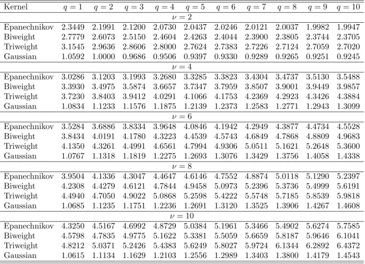
Table 1 provides the normal reference rule-of-thumb constants (C(kν) in (8)) for the νth-order
q-variate kernel density estimator (r = (0, . . . ,0)). The Biweight kernel corresponds to s= 2 and the Triweight kernel tos= 3 in ourspolynomial kernel family in (9). We point out several striking features. First, in the common setting of a second order kernel (ν= 2) the rule-of-thumb constants are decreasing as q increases. Scott (1992) notes that these reach a minimum when q = 11. The
ν = 2 case is the only one he considers. When ν >2,we see that the rule-of-thumb constants are increasing in the dimensionality of the problem. The basic idea behind this is given that higher-order kernels reduce bias, larger bandwidths are needed to minimize AMISE. However, note that the increase is not uniform over ν. For example, the optimal bandwidth for q = 2 and ν = 6 for the Gaussian kernel is 1.1318 and the rule-of-thumb bandwidth for that same kernel with ν = 8 is 1.1235. There appears to be an interplay between the roughness and variance which goes into calculating the rule-of-thumb bandwidth.
Table 1. Normal reference rule-of-thumb constants (C(kν)) for the multivariate
νth order kernel density estimator.
Kernel q= 1 q = 2 q= 3 q = 4 q= 5 q= 6 q = 7 q= 8 q = 9 q= 10 ν= 2 Epanechnikov 2.3449 2.1991 2.1200 2.0730 2.0437 2.0246 2.0121 2.0037 1.9982 1.9947 Biweight 2.7779 2.6073 2.5150 2.4604 2.4263 2.4044 2.3900 2.3805 2.3744 2.3705 Triweight 3.1545 2.9636 2.8606 2.8000 2.7624 2.7383 2.7226 2.7124 2.7059 2.7020 Gaussian 1.0592 1.0000 0.9686 0.9506 0.9397 0.9330 0.9289 0.9265 0.9251 0.9245 ν= 4 Epanechnikov 3.0286 3.1203 3.1993 3.2680 3.3285 3.3823 3.4304 3.4737 3.5130 3.5488 Biweight 3.3930 3.4975 3.5874 3.6657 3.7347 3.7959 3.8507 3.9001 3.9449 3.9857 Triweight 3.7230 3.8403 3.9412 4.0291 4.1066 4.1753 4.2369 4.2923 4.3426 4.3884 Gaussian 1.0834 1.1233 1.1576 1.1875 1.2139 1.2373 1.2583 1.2771 1.2943 1.3099 ν= 6 Epanechnikov 3.5284 3.6886 3.8334 3.9648 4.0846 4.1942 4.2949 4.3877 4.4734 4.5528 Biweight 3.8434 4.0191 4.1780 4.3223 4.4539 4.5743 4.6849 4.7868 4.8809 4.9683 Triweight 4.1350 4.3261 4.4991 4.6561 4.7994 4.9306 5.0511 5.1621 5.2648 5.3600 Gaussian 1.0767 1.1318 1.1819 1.2275 1.2693 1.3076 1.3429 1.3756 1.4058 1.4338 ν= 8 Epanechnikov 3.9504 4.1336 4.3047 4.4647 4.6146 4.7552 4.8874 5.0118 5.1290 5.2397 Biweight 4.2308 4.4279 4.6121 4.7844 4.9458 5.0973 5.2396 5.3736 5.4999 5.6191 Triweight 4.4940 4.7050 4.9022 5.0868 5.2598 5.4222 5.5748 5.7185 5.8539 5.9818 Gaussian 1.0685 1.1235 1.1751 1.2236 1.2691 1.3120 1.3525 1.3906 1.4267 1.4608 ν= 10 Epanechnikov 4.3250 4.5167 4.6992 4.8729 5.0384 5.1961 5.3466 5.4902 5.6274 5.7585 Biweight 4.5798 4.7835 4.9775 5.1622 5.3381 5.5059 5.6659 5.8187 5.9646 6.1041 Triweight 4.8212 5.0371 5.2426 5.4383 5.6249 5.8027 5.9724 6.1344 6.2892 6.4372 Gaussian 1.0615 1.1134 1.1629 1.2103 1.2556 1.2989 1.3403 1.3800 1.4179 1.4543
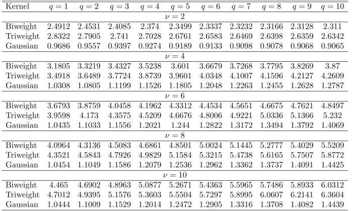
Table 2 provides the rule-of-thumb constants for the setting|r|= 1, which represents estimating a derivative of the multivariate kernel density estimator in a specific dimension. Here the normal
reference rule-of-thumb bandwidth can be shown to be (10) h|ROTr|=1= πq/22ν+q−1(ν!)2(q+ 2)R(kν)q−1R k(1)ν νκ2 ν(kν) [(2ν)!!(q+ν−1/2) + (q−1)2(ν!!)2] 1 2ν+2+q n−2ν+2+q1 .
We see exactly the same patterns for |r| = 1 as we did when |r| = 0. For 2nd order kernels the rule-of-thumb constants decrease for all kernels as the dimensionality increases while for higher order kernels the rule-of-thumb constants increase as the dimensionality increases. Note that Table 2 does not list rule-of-thumb constants for the class of Epanechnikov kernels as in this setting this kernel is not continuously differentiable over its support.
Table 2. Normal reference rule-of-thumb constants for the multivariate νth order kernel density derivative estimator for|r|= 1 provided in equation (10).
Kernel q = 1 q= 2 q = 3 q= 4 q= 5 q = 6 q= 7 q = 8 q = 9 q = 10 ν = 2 Biweight 2.4912 2.4531 2.4085 2.374 2.3499 2.3337 2.3232 2.3166 2.3128 2.311 Triweight 2.8322 2.7905 2.741 2.7028 2.6761 2.6583 2.6469 2.6398 2.6359 2.6342 Gaussian 0.9686 0.9557 0.9397 0.9274 0.9189 0.9133 0.9098 0.9078 0.9068 0.9065 ν = 4 Biweight 3.1805 3.3219 3.4327 3.5238 3.601 3.6679 3.7268 3.7795 3.8269 3.87 Triweight 3.4918 3.6489 3.7724 3.8739 3.9601 4.0348 4.1007 4.1596 4.2127 4.2609 Gaussian 1.0308 1.0805 1.1199 1.1526 1.1805 1.2048 1.2263 1.2455 1.2628 1.2787 ν = 6 Biweight 3.6793 3.8759 4.0458 4.1962 4.3312 4.4534 4.5651 4.6675 4.7621 4.8497 Triweight 3.9598 4.173 4.3575 4.5209 4.6676 4.8006 4.9221 5.0336 5.1366 5.232 Gaussian 1.0435 1.1033 1.1556 1.2021 1.244 1.2822 1.3172 1.3494 1.3792 1.4069 ν = 8 Biweight 4.0964 4.3136 4.5083 4.6861 4.8501 5.0024 5.1445 5.2777 5.4029 5.5209 Triweight 4.3521 4.5843 4.7926 4.9829 5.1584 5.3215 5.4738 5.6165 5.7507 5.8772 Gaussian 1.0454 1.1049 1.1586 1.2079 1.2536 1.2962 1.3362 1.3737 1.4091 1.4425 ν = 10 Biweight 4.465 4.6902 4.8963 5.0877 5.2671 5.4363 5.5965 5.7486 5.8933 6.0312 Triweight 4.7012 4.9395 5.1576 5.3603 5.5504 5.7297 5.8995 6.0607 6.2141 6.3604 Gaussian 1.0444 1.1009 1.1529 1.2014 1.2472 1.2905 1.3316 1.3708 1.4082 1.4439
References
Aldershof, B., Marron, J. S., Park, B. U. & Wand, M. P. (1995), ‘Facts about the Gaussian probability density function’,Applicable Analysis59(1), 289–306.
Cha´con, J. E., Duong, T. & Wand, M. P. (2010), Asymptotics for general multivariate kernel density derivative estimators. Working Paper.
Epanechnikov, V. A. (1969), ‘Nonparametric estimation of a multidimensional probability density’,Theory of Prob-ability and its Application14, 153–158.
Hansen, B. E. (2005), ‘Exact mean integrated squared error of higher order kernel estimators’,Econometric Theory
21, 1031–1057.
Hayfield, T. & Racine, J. S. (2008), ‘Nonparametric econometrics: The np package’,Journal of Statistical Software
27(5).
URL:http://www.jstatsoft.org/v27/i05/
Li, Q. & Racine, J. S. (2006),Nonparametric Econometrics: Theory and Practice, Princeton University Press, Prince-ton.
Li, T., Perrigne, I. & Vuong, Q. (2002), ‘Structural estimation of the affiliated private value auction model’,RAND Journal of Economics33, 171–193.
Masry, E. (1996), ‘Multivariate regression estimation: local polynomial fitting for time series’,Stochastic Processes and Their Applications65, 81–101.
Pagan, A. & Ullah, A. (1999),Nonparametric Econometrics, Cambridge University Press, Cambridge.
R Development Core Team (2008), R: A Language and Environment for Statistical Computing, R Foundation for Statistical Computing, Vienna, Austria. ISBN 3-900051-07-0.
URL:http://www.R-project.org
Scott, D. W. (1992),Multivariate density estimation: Theory, practice, and visualization, John Wiley and Sons, New York.
Silverman, B. W. (1986),Density estimation for statistics and data analysis, Chapman and Hall, New York. Wand, M. P. & Jones, M. C. (1993), ‘Comparison of smoothing parameterizations in bivariate kernel density
estima-tion’,Journal of the American Statistical Association88(422), 520–528.
Appendix A. Facts pertaining to the Gaussian probability density function
To obtain specific values for the normal reference rule-of-thumb bandwidths we need to invoke several properties of theq-variate normal probability density. The results presented here can either be found directly in Aldershof, Marron, Park & Wand (1995) and Wand & Jones (1993) or are straightforward extensions of their results.
The standard univariate normal probability density is defined as
φ(x) = (2π)−1e−(1/2)x2,
while the rth derivative of φ(x) is defined as
φ(r)(x) = (−1)rHr(x)φ(x),
whereHr(x) is the rth Hermite polynomial. The Hermite polynomials are defined as
Hr(x) =xHr−1(x)−(r−1)Hr−2(x), H0(x) = 1, H1(x) =x.
For the case where the random variable does not have unit variance the rescaling
φσ(x) =φ(x/σ)/σ
will be used. In this case therth derivative of φσ(x) is defined as
φ(σr)(x) =φ(r)(x/σ)/σr+1.
We will be interested in the rth derivative ofφσ(x) evaluated at 0. For this we have
φ(σr)(0) = (−1)r/2σ−(r+1)(2π)−1/2r!! forr even
and 0 otherwise.
In the multivariate setting we define the standardq-variate normal probability density as
φ(x) = q Y s=1 φ(xs) = (2π)−q/2e−(1/2)x 0x .
For Σ aq×q symmetric, positive definite matrix, we have
φΣ(x) =|Σ|−1/2φ(Σ−1/2x).
When Σ is diagonal with elementsσs2 we have
φΣ(x) =
q Y
s=1
φσs(xs).
Wand & Jones (1993, Theorem 2) show that for vectorsr= (r1, . . . , rq) and r0= (r10, . . . , rq0)
Z φ(Σr)(x)φ(r 0) Σ0 (x)dx=φ (r+r0) Σ+Σ0(0).
For the development of our normal reference rule we assume that Σ = Σ0 =Iq which yields Z φ(Ir) q (x)φ (r0) Iq (x)dx=φ (r+r0) 2Iq (0). Moreover, we have φ(2rI+r0) q (0) = q Y s=1 φ(√rs+rs0) 2 (0).
It is simple to check that whenr =r0 = (0, . . . ,0) we have
φ2Iq(0) =
q Y
s=1