Interactive visual exploration of overlapping similar structures for three-dimensional microscope images.

Author(s)

Nakao, Megumi; Takemoto, Shintaro; Sugiura, Tadao; Sawada,

Kazuaki; Kawakami, Ryosuke; Nemoto, Tomomi; Matsuda,

Tetsuya

Citation

BMC bioinformatics (2014), 15(1)

Issue Date

2014-12-19

URL

http://hdl.handle.net/2433/196840

Right

© 2014 Nakao et al.; licensee BioMed Central.

This is an Open Access article distributed under the terms of

the Creative Commons Attribution License

(http://creativecommons.org/licenses/by/4.0), which permits

unrestricted use, distribution, and reproduction in any medium,

provided the original work is properly credited. The Creative

Commons Public Domain Dedication waiver

(http://creativecommons.org/publicdomain/zero/1.0/) applies to

the data made available in this article, unless otherwise stated.

Type

Journal Article

Textversion

publisher

R E S E A R C H A R T I C L E

Open Access

Interactive visual exploration of overlapping

similar structures for three-dimensional

microscope images

Megumi Nakao

, Shintaro Takemoto

, Tadao Sugiura

, Kazuaki Sawada

, Ryosuke Kawakami

,

Tomomi Nemoto

and Tetsuya Matsuda

Abstract

Background:Recent advances in microscopy enable the acquisition of large numbers of tomographic images from living tissues. Three-dimensional microscope images are often displayed with volume rendering by adjusting the transfer functions. However, because the emissions from fluorescent materials and the optical properties based on point spread functions affect the imaging results, the intensity value can differ locally, even in the same structure. Further, images obtained from brain tissues contain a variety of neural structures such as dendrites and axons with complex crossings and overlapping linear structures. In these cases, the transfer functions previously used fail to optimize image generation, making it difficult to explore the connectivity of these tissues.

Results:This paper proposes an interactive visual exploration method by which the transfer functions are modified locally and interactively based on multidimensional features in the images. A direct editing interface is also provided to specify both the target region and structures with characteristic features, where all manual operations can be performed on the rendered image. This method is demonstrated using two-photon microscope images acquired from living mice, and is shown to be an effective method for interactive visual exploration of overlapping similar structures.

Conclusions:An interactive visualization method was introduced for local improvement of visualization by volume rendering in two-photon microscope images containing regions in which linear nerve structures crisscross in a complex manner. The proposed method is characterized by the localized multidimensional transfer function and interface where the parameters can be determined by the user to suit their particular visualization requirements.

Keywords:Interactive visualization, Multi-dimensional transfer functions, Neural structures, Microscopic images Background

Given the complex three-dimensional (3D) architecture of the brain, it is essential to explore the morphology and activity of neurons in all layers of the cortex. How-ever, this can often be challenging because the dendrites of cortical neurons are widely spread across several layers, including deeper layers that are difficult to ob-serve by confocal or light microscopy. The length of the dendrites can vary from 20 μm to 1 mm, and the width and branching of the dendrites depends on the distance from the soma. This suggests that spatial differences

in brain morphology relate to the functionality of the neuron, including characteristics of the dendrite and syn-aptic efficiency [1,2].

To understand the 3D structure of dendrites and the connectivity among neurons in the brain, in vivo im-aging and visualization have significant roles. Recently, the improved performance of microscopy systems has enabled the acquisition of large amounts of slice images from living tissues. In comparison with confocal or other optical microscopy systems, two-photon microscopy has an advantage in visualizing the morphology of neurons within deeper layers of a living mouse brain [3-6]. Be-cause the structures of tissues are stored as volume data, volume visualization techniques [7-9] are focused on the interactive exploration of the 3D images. When visualizing * Correspondence:[email protected]

†_{Equal contributors}

1

Graduate School of Informatics, Kyoto University, Yoshida Honmachi, Sakyo, Kyoto, Japan

Full list of author information is available at the end of the article

© 2015 Nakao et al.; licensee BioMed Central. This is an Open Access article distributed under the terms of the Creative Commons Attribution License (http://creativecommons.org/licenses/by/4.0), which permits unrestricted use, distribution, and reproduction in any medium, provided the original work is properly credited. The Creative Commons Public Domain Dedication waiver (http://creativecommons.org/publicdomain/zero/1.0/) applies to the data made available in this article, unless otherwise stated.

unknown features in the deeper layers of the brain, prior knowledge of the morphology of tissues [10,11] cannot be used. Furthermore, microscopic images are affected by op-tical characteristics such as scattering within tissues and the presence of image noise within the deeper regions of the images. Because large amounts of volume data are ob-tained through two-photon microscopy, there is a demand for efficient visualization of local internal structures and characteristic intensity distributions.

Direct volume rendering (DVR) has been widely used for visualizing volume data, where the rendered image is generated from the data by simulating optical properties such as radiation and absorption [12,13]. The user can interactively explore the micro-level structures included in the volume data while changing the camera parame-ters, modifying the transfer functions [14-16] or generat-ing the cross-section of the 3D images. Unlike the pattern recognition approach [17-19], visualization does not involve algorithm-based detection for specific ob-jects. In other words, the only aspects defined by the method are the transformations when visualizing the 3D image as a projection on the screen, and modifications of the visualization parameters and final judgments about the structures observed are left to the user.

The final quality of projections obtained with volume rendering depends significantly on the definition of the transfer functions (TFs). For this reason, the design of the TFs is regarded as an important area of research for volume visualization. Clinical tools commonly provide predefined TFs (TF presets) for efficiency in the clinical workflow. Recent studies have improved the TFs based on multidimensional feature values to visualize changes in texture and morphological characteristics included in the images [20-24]. Because the high degree of freedom in multidimensional TFs makes it difficult for users to obtain visualization results through manual parameter settings, a variety of user interfaces and automatic TF generation methods have been investigated [25-27]. In the case of visual exploration, there are many situations for which feature descriptors have not been formulated [28]. Some researchers have focused on this issue and have investigated methods for exploring high-dimensional feature space. Principal component analysis, independent component analysis, and clustering techniques are com-monly used for dimensionality reduction of the feature space [29,30].

In microscope images, the intensity value of voxels can differ locally, even within the same structure, be-cause emission of fluorescent materials and the optical properties based on point spread functions affect the im-aging results. Most previous TFs designed for clinical computed tomography (CT) and magnetic resonance imaging (MRI) images are not applicable to images that have specific areas with locally varying contrast. In

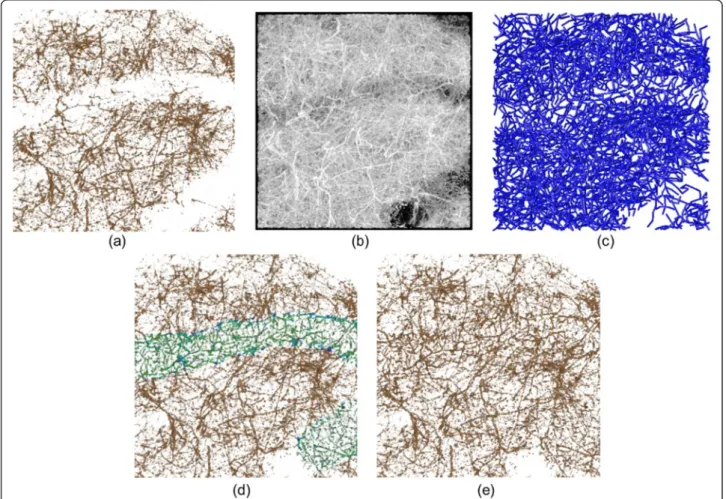
addition, images obtained from brain tissue contain a var-iety of neural structures such as dendrites and white matter, where similar line structures are overlapped or crisscrossed with some complexity (see Figure 1). Numer-ous minute or thin structures can be closely observed with optical scattering noise. In these cases, previous TFs often fail to optimize the visualization results, making it difficult to explore the connectivity of neurons because of their oc-clusions and geometric complexity. The main focus of this study, therefore, is to answer these issues in biological visualization, and to design an efficient visual exploration tool.

This paper proposes an interactive visual exploration method by which the TFs are modified locally and inter-actively based on multidimensional features of the images. This method will also provide a direct editing interface to specify both the target region and the structures with characteristic features, where all manual operations can be performed on the rendered image. Therefore, multidimen-sional features and interactive methods can be used for local improvement of the visualization results for overlap-ping structures. Despite the high dimensionality of the TFs, users only specify the structures of interest on the rendered image and control simple parameters to explore similar structures. The performance of the method is demonstrated using two-photon microscope images mea-sured from live mice. The experiments show that this method is effective for interactive visual exploration of overlapping similar structures.

Regarding related study in vessel visualization, the re-cent work by Kubisch et al. [31] summarizes problems and reviews of related work. Much recent work has fo-cused on multi-scale methods based on eigenvalue ana-lysis of the Hessian [18]. Using the vesselness measure, Lathen et al. [27] presented automatic tuning techniques by applying a locally shifted intensity to the TFs (called a TF shift) in the vessel visualization domain. In computed tomography angiography (CTA), which is analogous to microscope images, the intensity value of blood vessels partially decrease owing to the distribution deflection of the contrast medium. The advantage of this approach is to use the 1D TF presets that are popular in clinical applica-tions and are easily set up in a visualization workflow.

In this study, we consider an application of the TF shift technique to 3D microscope images. In biological visualization using two-photon or confocal microscope im-ages, however, the main focus is on neural structures that crisscross in a complex way with multiple overlaps. The deep layers of the brain tissue contain a variety of neural structures with complex shapes such as soma, dendrites, and white matter. Unlike the situation that exists in clinical CT or MRI images, however, numerous minute or thin structures are closely observed with optical scattering noise, which creates challenges for volume visualization. To our

knowledge there have been no reports on an interactive, visual exploration software and interface for overlapping similar neural structures in microscope images. This study proposes a new TF shift mechanism and interface that can efficiently use more general multidimensional feature values, while avoiding a complex TF design process. Methods

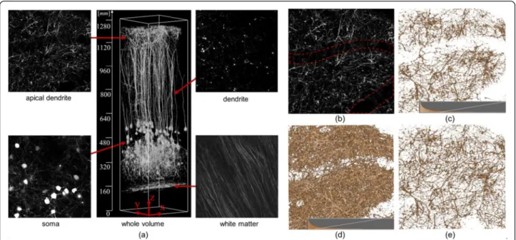
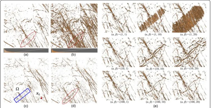
Figure 1 shows slice images that include structures with characteristic shapes measured from a live mouse using a two-photon microscope. The central image shows the results of visualization of the entire image data with an intensity-based 1D TF. Apical dendrites, dendrites, soma, and white matter, which are all parts of the neu-rons, are included in the images. In the apical dendritic region, linear structures run along thexyplane and each linear structure crisscrosses in a complex manner. The large linear shadow shown within the red frame in the middle of the image indicates blood vessels, because there is a tendency for a decrease in the intensity value of structures directly below blood vessels. In the den-dritic regions, linear structures with a high intensity value can be found along the z axis and, around these, linear structures with low intensity values exist in large quantities, though these structures are not visible. The soma can be identified as a spherical structure. In the white matter region, most of the linear structures run in the specific direction of thexyplane.

We will now discuss our goals toward visualization in the microscope images. Figure 1(b) is a tomographic

image of apical dendrites located near the brain surface. However, there is actually a large quantity of low lumi-nance neurons around the dendrites, making observa-tion of the dendrites difficult. Blood vessels with a diameter of ~30 voxels run within this data, and are seen as regions in which nerves do not exist. The low contrast area shadowed by the blood vessels is shown within the red frame in Figure 1(b). Figure 1(c) and (d) shows the volume visualization results obtained by a traditional intensity-based 1D TF. The histogram of the voxel and the opacity curve setting in the TF is inserted in the bottom of each figure. In Figure 1(c), it is not pos-sible to distinguish most of the structures with low in-tensity under the area of blood vessels. Figure 1(d) shows another visualization result obtained by adjusting the window level parameter of the TF to a lower level. In this figure, some structures can be observed in the low contrast area. However, because of a widening in the range of opaque intensity, surrounding dendric structures and optical noises can occlude the target structure, which fails to distinguish the connectivity of the three-dimensional neural networks. Figure 1(e) is a visualization result obtained by the method proposed in this study, which succeeds in distinguishing dendric structures and their connectivity under the blood ves-sels. Because the color/opacity outside the target area does not change, the target structures with low intensity as well as the other structures outside of the region of interest can be seen simultaneously without self-occlusion or noise enhancement.

Figure 1Visual exploration of overlapping neural structures. (a)An example of three-dimensional microscope images with a depth ~1.3 mm from the surface layer of the cortex.(b)Tomographic image of apical dendrites. The low contrast area shadowed by the blood vessels is shown within the red dashed lines. Volume visualization results obtained by(c) (d)a traditional intensity-based 1D TFs and(e)the proposed method, which succeeds in locally improving the visualization result.

Here, we describe a set of methods to achieve the above-mentioned local refinement of the rendered image. Because intensity values and contrast can differ locally in the target data of this study, the method developed by Lathen et al. for CTA images [27] is used as a basis for the local adjustment of TFs. To achieve automatic tuning of visualization results for linear structures, Lathen et al. employed thevesselnessmeasure as feature values. In our study, for visualization of various neural structures such as soma, dendrites, and apical dendrites with different fea-tures and sizes, we design a novel TF shift framework to address these multidimensional feature values. In addition, for efficient visualization of dendric structures that criss-cross in a complex manner, locally similar structures are selectively visualized by direct editing of the visualization results on the rendered image.

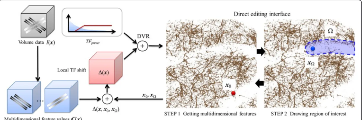
Flowcharts of the proposed method are shown in Figure 2. With the proposed method, a predefined 1D TF (TFpreset) is first prepared, and DVR of the target data is

conducted. The colored histogram with a linear graph at the bottom of Figure 1(c) and (d) is used as a TF set-ting interface, which is a common interface in medical visualization software. The user can change the color lookup table that maps the intensity to RGBA values on the histogram. Opacity values are defined using the linear graph or using free form curves manually drawn by the user. These configurations can be done by mouse oper-ation only. In addition to modifying TFs, users can obtain desired visualization results based on the rendered im-ages. Users can directly specify the structures of interest

Ω∈R3as visualization targets. During visualization work-flow, users input into the system one point of a structure (x0) similar to the structures of interest such thatx0∈R3, and the central coordinate of differentialΩ(xΩ). Our

sys-tem calculates the shift value (Δ) of the TF of all voxel

positions (x) within Ωon the basis of xΩand x0. Then,

the input for the TF is modified, and DVR is again proc-essed. If users are not satisfied with the rendering results, the TF can be modified again.

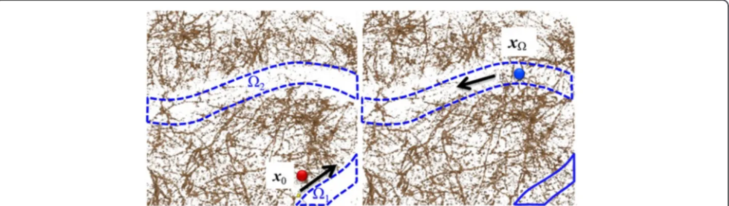
Figure 3 shows changes in visualization when x0 is fixed andΩis altered, along with the shift valueΔof the TF. In this case, the shape of the 3D pointer is a sphere, which works as a minimal ROI for the local TF shift. The radius of the pointer is changed by the user, and the time series input by dragging a mouse defines the total ROIΩ. Therefore, the shape of the ROI can be modified interactively and can be any form. By increasing the shift value of the TF in low-intensity voxels, if there is a simi-lar structure one can assume the visualization results to be the same, regardless of the intensity value. The TF configured by the user is stored in a file to be re-used by different users or the same user at different times. Be-cause the TFs consist of volumetric, spatially-varying scalar values, the file format can be the same as three-dimensional image format.

Localized multidimensional transfer function

This section describes details of the designed spatially varying TF based on multidimensional feature values. In a method similar to the approach used by Lathen et al. [27], our system uses a basic objective function based on the Eq. (1)

T Fðx; Ið Þx ;Δð Þx Þ ¼ T FpresetðIð Þ þx Δð Þx Þ; ð1Þ

where I is the intensity distribution of the volume data.

For selective visualization of a variety of structures contained in a microscope image, the design of the cal-culation formula of the shift valueΔof the TF becomes

Figure 2Flowchart and user interface of the proposed visualization framework.Multidimensional feature values of microscope images are addressed in visualization process with local TF shift. With the direct editing interface, the user can explore overlapping similar structures with spatially different contrast locally and interactively.

important. Specifically, unlike the previous TF shift technique based on the vesselness measure, multidimen-sional features are addressed in our framework. The fol-lowing section explains the concrete calculation formula ofΔ. In addition, to allow users to interactively input x0 andxΩinto the system, it is essential to develop a method

for inputting 3D coordinates on the rendering image. The calculation formula of Δ is designed to meet Conditions (A), (B), and (C), given as

(A) IfI(x) =I(x0), thenRGBA(x) =RGBA(x0).

(B) IfC(x)≈C(x0),RGBA(x)≈RGBA(x0).

(C) OnlyRGBA(x) changes within the regionΩnearxΩ.

In these conditions, the color/opacity value of pointx is expressed asRGBA(x), and the feature value of point

xis expressed asC(x)∈Rn.

Condition (A) is used to maintain the integrity of the cal-culation. In the proposed method, reference point x0 can also become a processing target. For the situation where there is no shift in the TF of the reference pointx0, Condi-tion (A) must be feasible. CondiCondi-tion (B) indicates that the color/opacity value of structures similar tox0changes. If the features are similar, even with structures of different lumi-nance, visualization can be achieved on the basis of the color/opacity value previously determined with TFpreset.

Condition (C) indicates that only the color/opacity value in the region Ω specified by the user changes. Visualization that maintains visibility can be achieved through spatial and local visualization when structures with multiple over-laps are not portrayed. To satisfy Condition (A), the shift function Δ(x, x0, xΩ) should have I(x0)−I(x) as a factor. Introducing the functiong(x,x0, xΩ) where (1≥g≥0),Δis determined as

Δðx;x0;xΩÞ ¼ðIð Þx0 −Ið Þx Þgðx;x0;xΩÞ: ð2Þ When g= 1, then Δ=I(x0)−I(x) and TFpreset becomes TFpreset(I(x0)). This means that the color/opacity value

RGBA(x) in x becomes the same as RGBA(x0) in x0. When g= 0, then Δ= 0, and the color/opacity value

RGBA(x) of x is unchanged. To achieve Condition (B), the dissimilarity of C(x) andC(x0) (dF(C(x),C(x0)) where

(dF> 0)) in the feature value space is calculated. A larger dFrelates to a greater difference in the features of

struc-tures in x and x0. The Mahalanobis distance and inner product can be used in the calculation ofdF. Equation (5)

shows cases in which the Mahalanobis distance dmah is

used in Eq. (3), and when the inner product ddot is used

in Eq. (4). dmahðC xð Þ;C x0ð ÞÞ ¼ ffiffiffiffiffiffiffiffiffiffiffiffiffiffiffiffiffiffiffiffiffiffiffiffiffiffiffiffiffiffiffiffiffiffiffiffiffiffiffiffiffiffiffiffiffiffiffiffiffiffiffiffiffiffiffiffiffiffiffiffiffiffiffiffiffiffiffi C xð Þ−C x0ð Þ ð ÞT_V−1_{ðC xð Þ−C x0ð ÞÞ} q ; ð3Þ ddotðC xð Þ;C xð Þ0 Þ ¼1−C xð Þ⋅C xð Þ0 ; ð4Þ where C(x) is the feature value vector at x and V is the covariance matrix between every feature value. To achieve Condition (C), the distance ofxand x_Ωis calcu-lated in the virtual space by the Euclidean distance

dE(x,xΩ) where (dE> 0). When considering the functiong

(x,x0,xΩ) that satisfies Conditions (B) and (C), g is first

defined, as with Eq. (5). Next, the function fF, which

changes in value according to the dissimilarity of features, and the functionfE, which determines the range of Ω, are

introduced as

gðx;x0;xΩÞ ¼fFðdFðx;x0ÞÞfEðdEðx;xΩÞÞ: ð5Þ

To satisfy 1≥g≥0,fFand fEmust each satisfy 1≥fF≥0

and 1≥fE ≥0. Function fF, which satisfies Condition (B),

and the sigmoid functionfE, which satisfies Condition (C),

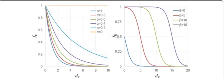
are shown in Eqs. (6) and (7), respectively. An outline of these functions is given in Figure 4. By using the sigmoid function infE, the visualization results at the boundaries of Ωcan be easily changed, and improvement in visualization quality can be expected.

f_Fð Þ ¼dF e−αdF; ð6Þ

Figure 3Interactive editing of the visualization results.By locally changing the shift value of the TF in the low-luminance area, similar structures with low intensity values can be visualized based on multidimensional features.

f_Eð Þ ¼dE 1

1þedE−β; ð7Þ where the configurable parametersα≥0 and β≥0 are introduced by the user. Parameter α is the sensitivity that determines the amount of the change in RGBA

dependent on the dissimilarity of the feature values. Parameter β is the radius that determines the size of regionΩ. The shift valueΔwhenfFand fE from Eqs. (2),

(6), and (7) are used is given as

Δðx;x0;xΩÞ ¼ðIð Þx0 −Ið Þx Þ e−αdF

1þedE−β: ð8Þ

Direct editing interface

In this section, we consider the method for directly in-putting the 3D coordinatesx0and xΩonto the rendered

image. With the volume rendering process, volume data are projected in the viewing direction νeye∈R

3

. As such, there are voxels drawn by the click point (xclick∈R2) of

the rendered image in the direction ofνeye, which

origi-nates from xclick. Among the quantity of voxels existing

in the direction of νeye, those close to the surface of the

structure are believed to be the voxels specified by the user and are estimated using degrees of transparency [32,33]. First, the volume data are searched from the

xclick point in the direction of νeye. During the search,

voxels are sampled at fixed intervals, xi. Next, the sum

Xn

i¼0αi of the opacity value (αi) of xiis calculated. The

value of αi is calculated using TF(x, I(x), Δ(x)), which

considersΔ. The voxel is acquired that is larger than a threshold opacity value (αth) predefined by

Xn

i¼0αi, and

these voxels are assumed to be those specified by the

user and are close to the surface of the structure that has been visualized to consider theΔ.

Results and discussion

We implement a sequence of algorithms using C++, OpenGL, GLSL (Open GL Shader Language), and the software package NVIDIA CUDA (Compute Unified Device Architecture). We apply the developed software to two-photon microscope images and verify the visualization of the characteristic structures and the intensity distri-bution included in the images with biological researchers. For the 3D microscope image and for visualization of its feature volume, we use the texture-based rendering scheme [13] to achieve high-speed volume rendering using the texture interpolation and synthesis functions of the graphics processing unit. For verification, we used three volume data sets taken from live, genetically modi-fied mice [4] using a Nikon two-photon microscope (A1MP+), wherein the neurons in the second and fifth layers of the mouse cortex are labeled by a green fluores-cent protein. The study was carried out in accordance with the recommendations in the Guidelines for the Care and Use of Laboratory Animals of the Animal Research Committee. The protocol was approved by the Committee on the Ethics of Animal Experiments. These data sets capture a tomogram with a depth ~1.4 mm from the surface layer of the cortex. The volume data have a size of 512 × 512 × 325 voxels, and the range of capture is 512 × 512 × 1300μm. Neurons are included within the image, and the direction from the deep part of the brain toward the brain surface is assigned as the posi-tive zaxis. Apical dendrites, dendrites, soma, and white matter exist in the positivez direction. To reduce noise,

Figure 4Two sub-functionsfFandfEdefined by the configurable parameters, where the parameterαis the sensitivity that determines the amount of the change in RGBA dependent on the dissimilarity of the feature values and parameterβis the radius of the current region ofΩ.

a median filter is applied for preprocessing the volume data.

For this experiment, the ratios of the eigenvalues λ1, λ2, and λ3of the Hessian matrix and the eigenvector e3 belonging to the third eigenvalue of the Hessian matrix are used to express the shape feature. The feature value λratio, which highlights linear structures, is calculated

fromλ1,λ2,andλ3based on

λratio¼ λ2=λλ12−=λλ13=λ1 0 λ1≤λ2≤λ3≤0 ð Þ λ1≤λ2≤0;λ3>0 ð Þ otherwise 8 < : ð9Þ

Voxels with large λ2/λ1 ratios are linear or spherical local structures, whereas those with large λ3/λ1 ratios are spherical local structures. As such, voxels with a large difference value for λ2/λ1−λ3/λ1 are linear local structures. In addition, linear structures with an intensity less than that of the background have positive values of λ1 and λ2, whereas those with an intensity greater than that of the background have negative λ1and λ2 values. Because the linear structures included in the target data of the present experiment have an intensity value greater than that of the background, λratio is prevented from

becoming increased (in voxels) with an intensity less than that of the background by using the conditions

λ1≤λ2≤λ3≤0 andλ1≤λ2≤0,λ3> 0. The feature value

e′3, which corrects the eigenvectore3, is given as

e0

3¼ e₀3 ð_ðλ_otherwise1≤λ2≤0_ÞÞ

ð10Þ

As with e′3 and λratio, and by using the condition

λ1≤λ2≤0, e′3 is prevented from having a value in voxels with an intensity less than that of the background.

White matter

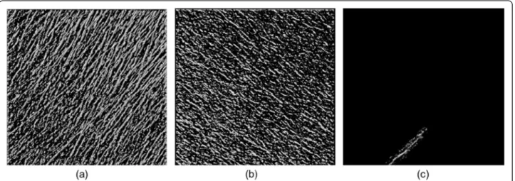
During the experiment, the region containing white mat-ter is trimmed, andνeyeat the time of rendering is set as

the−zdirection. Figure 5(a) and (b) shows visualization results with 1D TF presets. We are able to confirm that most of the linear structures are included within the image in the (x, y, z) = (1, 1, 0) direction, but linear structures in directions other than (1, 1, 0) also exist but cannot be visualized clearly. Here, the focus is on linear structures in the direction (1, −1, 0) within the red circle. In the visualization of Figure 5(a), many parts of the linear structures in the red frame have become transparent. In Figure 5(b), linear structures in the (1, 1, 0) direction occlude the structures within the red frame, making it difficult to distinguish them. We attempt to se-lectively visualize based on the orientation of the linear structures by using e′3 as the feature. Because e′3

Figure 5Interactive visual exploration for overlapping white matter structures.Visualization results obtained using(a)and(b)1D TF presets,(c)x0andΩset by the user,(d)the locally refined result and(e)effect of the configurable parametersαandβ, wherein the sensitivity

represents the local orientation of the structure, it is better to use the inner product rather than the distance when calculating the dissimilarity dF. The expression for dF in

this case is given as

dFðx;x0Þ ¼1−e03ð Þx ⋅e03ð Þx0 : ð11Þ The TFpreset used in Figure 5(a) is used for our

method, and the structure already visualized is indicated as a feature point. The x0andΩare set as shown in (c). The results of the interactive visual exploration with α= 10 and β= 6 are shown in (d). Compared with the visualization results obtained with 1D TF presets (Figure 5(a) and (b)), the results obtained with our method (Figure 5(d)) present the existence of structures within the red frame that are easily distinguished by users

We now qualitatively examine the process of visualization by the proposed method by first discussing the valid-ity of the calculated dF. The value of the feature at x0 is e′3(x0) = (−0.847, 0.527, 0.0650). The results of the visualization of all voxels having the dissimilarity of the feature withdF≤0.5 are shown in Figure 6(a). The

struc-tures visualized in (a) are those in which the angle with

e′3(x0) is within 60°. Figure 6(b) displays the vector

e′3⊥(x0), which is perpendicular to e′3(x0) in the xy plane, showing the visualization results of all voxels with

dF≤0.5, and structures in which the angle withe′3⊥(x0) is within 60° are visualized. By calculatingdFwith the feature

60°, we find that each linear structure in a different direc-tion can be separated. With the proposed method, the visualized area is limited by visualizing structures only within Ω after separating the visualization target struc-tures from other strucstruc-tures by usingdF. Figure 6(c) shows

the shiftΔof the TF when the proposed method is tested with α= 10 and β= 6. Structures around the computer

mouse cursor are visualized during the operation. Users can use the visualized structures as a guide and can inter-actively specify these structures targeted for visualization. We see that only TFs of the target structures can be modi-fied by using dFwithin the visualized region Ω.

Further-more, the average frames per second for visualization is 53, confirming that the proposed method is interactive in practice.

Next, we examine the effect of the sensitivity αand the radius βon the visualization results. The parameters are varied so thatα= 1, 10, and 100 andβ= 1, 10, and 20, and the results of visualization by combining each of these values are shown in Figure 5(e). Whenα= 1, structures are completely visualized except for the background; whenα= 10, linear structures in the (1, −1, 0) direction are visual-ized; and when α= 100, the visualization results are the same before and after the operation. When the focus is on visualizing similar structures of x0, a suitable parameter value forαwhich enables visualization of linear structures in the direction (1,−1, 0) isα= 10. Whenαis larger than this value, it is not possible to visualize targeted structures, and whenαis smaller than this value, structures outside of those targeted are visualized. Next, when β= 1, the visualization results before and after the operation are prac-tically unchanged. Whenβ= 10, both the target structures and surrounding structures are visualized, and whenβ= 20, structures corresponding to a wider range thanβ= 10 are visualized. Thus, to visualize the target structures only, it is best to use the smallest β possible. However, if β is too small, the function cannot be used as a guide when specify-ing the target structures. Conversely, although it is easy to specify target structures ifβis large, it is possible that struc-tures outside of those targeted may also be visualized.

As such, it is necessary to select suitable parameters based on user objectives and on the actual situation

Figure 6Three-dimensional TF shift distribution globally computed based on (a) the orientation of the structures, (b) vertically overlapping structures and (c) locally selected by the user.

when attempting to obtain good visualization results. Although the parameters are modulated based on a trial-and-error process, the following guidelines can be considered. Becauseαcontrols sensitivity of the features that are to be visualized, largeαvalues are first suitable to roughly visualize local structures with a variety of fea-tures, and then smaller values can be tried to strictly ex-tract the target features.βcontrols the size of the direct editing pointer that defines the minimal region of inter-est (ROI). Therefore,βcan be adjusted based on the size of the target structures. Largerβis useful when search-ing non-visualized, transparent structures existsearch-ing within the volume data. After visualizing a part of the target structure, a small βis useful for fine adjustment of the visualization results.

Dendrites

Next, we apply this method to the area with dendric structures. The eye direction (νeye) during volume

ren-dering is set as +z. Figure 7(a) shows volume rendering results obtained with 1D TFs, which fails to visualize thin dendric structures with lower intensities. Here, we focus on visual exploration of the local area A and B. Figure 7(b) is visualized using previous method, in which we modify the TFs of the area based on the vesselness

measure used by Lathen et al. [27] for the feature. Linear

structures of low intensity appear and run over the xy

plane around the dendrites, but only some of the struc-tures can be distinguished. Because all linear strucstruc-tures in the data are highlighted as shown in Figure 7(c), it is hard to present the endpoints of one linear structure in a form visible to the eye. By applying the proposed method to this dendritic region, we attempt to observe structures in detail. Equation (10) andλratioare used for

the feature to highlight the linear structures. The expres-sion used in this experiment is given:

dFðx;x0Þ ¼ 1 σ ffiffiffiffiffiffiffiffiffiffiffiffiffiffiffiffiffiffiffiffiffiffiffiffiffiffiffiffiffiffiffiffiffiffiffiffiffiffiffiffiffiffi λratioð Þx −λratioð Þx0 ð Þ2 q ð12Þ

where the quantityσis the standard deviation ofλratio.

The point of the linear structures is denoted asx0. To apply small modifications to the visualization results, we use (α,β) = (0.30, 6). By changing the specified region of

Ω, we interactively obtain the visualization result. First, clear structures are visualized among the linear structures when the dendrites within the area B are taken as the start-ing point. The proposed method enables the presentation of plural structures in forms distinguishable to the eye, which are difficult to observe in semitransparency with methods developed to date. In addition, when using the

vesselness measure based TF shift, many overlapping

Figure 7Comparison between the vessel measure based TF shift[27]and the proposed interactive exploration. (a)1D TF preset visualization,(b)close-up visualization of the area A and B shifted by the vesselness measure,(c)the TF shift applied to the area,(d)interactive editing results by the proposed framework for tracing specific dendric structures with lower intensity and(e)the TF shift.

structures are displayed simultaneously. However, the pro-posed method allows the structures of interest to be traced easily on the rendered image. Figure 7(d) shows the visualization results after interactive editing of the dendric structures. The TF shift is shown in Figure 7(e). Compar-ing the two methods, linear structures that are largely transparent and cannot be distinguished can be visualized using the proposed method.

Apical dendrites

Finally, a visualization experiment targeting the apical dendritic region is performed. We applied our data to the Vaa3D visualization software employing virtual fin-ger (VF) techniques [7,8] and compared the visualization results. We tried the visualization functions and the tra-cing tool in the Vaa3D software, and finally decided to focus on the two functions of MIP (maximum intensity projection) based direct volume rendering (DVR) and Vaa3D-Neuron2 auto-tracing for comparison with our local TF shift techniques. Our visualization targets are the dendric structures possessing a lower intensity located

under the blood vessels. Although there are linear dendric structures that cross the blood vessels in Figure 8(a), their connectivity and distribution are not clear with the 1D preset TF.

Figure 8(b) shows the MIP-based DVR results in the Vaa3D software. This rendering mode is effective for visualizing occluded vessels, and some neural structures can actually be observed in the lower intensity area. However, because of a widening in the range of opaque intensity, optical noise or unfocused surrounding struc-tures are also visualized globally, which can decrease the contrast between the neural structures and back-ground areas. This continues to make it difficult to clearly visualize connectivity of the neural structures. Figure 8(c) shows the Vaa3D-Neuron2 auto-tracing result with an auto-thresholding mode [8]. Neural structures are recon-structed as surface models by correcting imperfect parts in the traced areas. However, this function can yield many artifacts, especially around complex crossing structures with low-contrast intensity values. When higher threshold values are used, the artifacts can be reduced but

Figure 8Apical dendric region represented using (a) TF preset visualization, (b) MIP-based DVR, (c) surface reconstruction by neuron tracing, (d) TF shift applied to the low contrast area locally and interactively and (e) the improved DVR result, which clarifies the connectivity of neural structures.

reconstruction of the neural structures in low intensity area is not achieved. This results in a difference in the spatial density of neural structures in low-intensity areas and in other areas. We also note that the tracing result is represented using the reconstructed surface models. Lo-cally improved DVR is not achieved using only vessel tra-cing tools.

With the proposed method, the TF shift is applied to the low-intensity area locally and interactively. The pa-rameters used in this experiment are (α, β) = (0.45, 20). Figure 8(d) shows the spatial relationship between the TF shift applied to a low-intensity area and other dend-ric structures with high intensity. Figure 8(e) is the final rendering result, and the connectivity of the dendric structures can be viewed thanks to locally improved DVR images. Compared with (a), (b) and (c) of Figure 8, the visual appearance of the spatial density for vessel structures is corrected, which generates a more natural visualization result in (e). Thus, our approach can simul-taneously visualize regions that are below blood vessels without affecting regions that are not.

Discussion

So far, most interaction techniques [7,8,32] assume that the entire shapes of the target structures is first visual-ized in the screen. Then, by pinpointing a 3D position on the rendered image, the user can extract a part of the 3D structure to specify his/her ROI. However, microscopic images obtained from brain tissues some-times contain a variety of neural structures with com-plex crossings and overlapping linear structures. In these cases, even if the 3D location is specified, the tracing task is difficult and often fails to extract a single linear struc-ture because undesired surrounding strucstruc-tures are simul-taneously selected. In the developed software, we can start the tracing task on the partially-visualized struc-ture and can expand it to transparent regions with low-intensity areas where no structures are yet visualized (see Figure 3). In addition, thanks to the multidimen-sional TF, the user can limit the visible structures in a ro-bust way based upon a combination of 3D features such as direction, radius and textures (Figures 6, 7 and 8). The multidimensional TF design and its combination with the direct editing interface are main contributions of this work in biological visualization. In addition, three-dimensional images with scalar intensity values measured from electron microscopes and confocal microscopes as well as CT/MRI images can be applied to our software. We will further study practical application to other types of volume data

The automation of transfer function (TF) generation is a critical issue in volume rendering. Specifically, in bio-logical volume visualization, users often focus on over-lapped neural structures or internal structures occluded

by other surrounding tissues. When automatic TF tuning [26,27] is applied globally, many structures are simultan-eously visualized and some of these structures occlude the target structures. In Figure 7(c), because similar structures in the data are highlighted, it is difficult to present the endpoints of one linear structure in a visually distinguish-able form. Applying machine learning or clustering ap-proaches [28] are interesting methods to automate TF configuration, but they require prior knowledge to learn the target structures.

Knowledge exploration for newly-measured data is regarded as a user-dependent problem in many situations. The advantage of the interactive, manual TF configuration is that features of interest can be locally explored based on the user's preferences. This user-dependent localization of information visualization is an important factor to transfer the user's biological knowledge into the visualization sys-tem. Also, because the developed system does not require any time-consuming setup, it can provide a practical en-vironment for rapid visualization of the measured data. Combining the interactive localization with automatic TF tuning would be interesting and has the possibility of a more intelligent interface for volume visualization, and we would like to further study this on the semi-automatic framework.

Conclusions

In this study, a method is proposed for interactive and local improvement of visualization by volume rendering in two-photon microscope images containing regions in which linear nerve structures crisscross in a complex manner. For this method, multidimensional features and interactive methods are used for selectively visualizing structures. Users can specify the structures and regions of interest on the rendered image and only visualize similar structures in the regions of interest. The pro-posed method introduces the parametersαandβ, which are freely tuned by the user. The sensitivityαdetermines how easy it is to change visualization results by similarity, whereas the radiusβdetermines the size of the region of interest.

By applying the proposed method to an image of a mouse brain acquired by two-photon microscopy, we visualize white matter, dendrites, and apical dendrites in which we verify the proposed method in an experiment in the region containing white matter. The proposed method is characterized by multidimensional features and interactive methods that are effective for visualizing target structures. Furthermore, we investigate the effect of parameters α and β on the results of visualization, where we find that a large β is suitable for search pur-poses and a smallerβis effective for small modifications of the visualization results. Because the suitable values of α and β depend on the situation, the proposed

method promises that visualization can be implemented with flexibility, and that the parameters can be deter-mined by the user to suit their particular visualization requirements.

Availability of supporting data

The data sets supporting the results of this article are in-cluded within the article.

Competing interests

The authors declare that they have no competing interests.

Authors_’contributions

MN carried out design of the study, the implementation of the software and a part of the experiments. ST participated in the implementation of software, feature analysis and a part of the experiments. TS conceived of the study and participated in the measurement of the mouse brain data. KS carried out measurement of the mouse brain data. RK participated in development of the two-photon microscopy and evaluation of the software. TN participated in development of the two-photon microscopy and evaluation of the software. TM carried out design of the study and participated in its design and coordination. All authors read and approved the final manuscript.

Acknowledgements

This work was supported by Platform for Dynamic Approaches to Living System from the Ministry of Education, Culture, Sports, Science and Technology, Japan. This research was also supported by a Japan Society for the Promotion of Science (JSPS), Grant-in-Aid for Scientific Research for Young Scientists, Number 24680059.

Author details

1

Graduate School of Informatics, Kyoto University, Yoshida Honmachi, Sakyo, Kyoto, Japan.2_{Graduate School of Information Science, Nara Institute of}

Science and Technology, 8916-5, Takayama, Ikoma, Nara, Japan.3Graduate School of Information Science and Technology, Hokkaido University, Sapporo, Hokkaido, Japan.4Research Institute for Electronic Science, Hokkaido University, Sapporo, Japan.

Received: 30 July 2014 Accepted: 9 December 2014

References

1. Matsuzaki M, Honkura N, Ellis-Davies GC, Kasai H:Structural basis of long-term potentiation in single dendritic spines.Nature2004,

429:761–766.

2. Nicholson DA, Trana R, Katz Y, Kath WL, Spruston N, Geinisman Y:

Distance-dependent differences in synapse number and AMPA receptor expression in hippocampal CA1 pyramidal neurons.Neuron2006,

50:431–442.

3. Nakashiba T, Cushman JD, Pelkey KA, Renaudineau S, Buhl DL, McHugh TJ, Rodriguez Barrera V, Chittajallu R, Iwamoto KS, McBain CJ, Fanselow MS, Tonegawa S:Young dentate granule cells mediate pattern separation, whereas old granule cells facilitate pattern completion.Cell2012,

149:188–201.

4. Kawakami R, Sawada K, Sato A, Hibi T, Kozawa Y, Sato S Yokoyama H, Nemoto T:Visualizing hippocampal neurons with in vivo two-photon microscopy using a 1030 Nm picosecond pulse laser.

Sci Rep2013,3.

5. Pan F, Gan WB:Two-photon imaging of dendritic spine development in the mouse cortex.Dev Neurobiology2008,68:771–778.

6. Trachtenberg JT, Chen BE, Knott GW, Feng G, Sanes JR, Welker E, Svoboda K:Long-term in vivo imaging of experience-dependent synaptic plasticity in adult cortex.Nature2002,

420:788–794.

7. Peng H, Ruan Z, Long F, Simpson JH, Myers EW:V3D enables real-time 3D visualization and quantitative analysis of large-scale biological image data sets.Nature Biotec2010,28(4):348–353.

8. Peng H, Tang J, Xiao H, Bria A, Zhou J, Butler V, Zhou Z, Gonzalez-Bellido PT, Oh SW, Chen J, Mitra A, Tsien RW, Zeng H, Ascoli GA, Iannello G, Hawrylycz M,

Myers E, Long F:Virtual finger boosts three-dimensional imaging and microsurgery as well as terabyte volume image visualization and analysis.

Nat Commun2014,5. http://dx.doi.org/10.1038/ncomms5342

9. Wan Y, Otsuna H, Chien C, Hansen C:An interactive visualization tool for multi-channel confocal microscopy data in neurobiology research.IEEE Trans Visual Compute Graphics2009,15(6):1489–1496.

10. Heinmann T, Meinzer HP:Statistical shape models for 3D medical image segmentation: a review.Med Image Analysis2009,

13(4):543–563.

11. Guerrero R, Wolz R, Rueckert D:Laplacian eigenmaps manifold learning for landmark localization in brain MR images.Med Imaging Comput Comput-Assist Interven2011, 566-573

12. Levoy M:Efficient ray-tracing of volume data.ACM Trans Graphics1990,

9(3):256–261.

13. Cabral B, Cam N, Foran J:Accelerated volume rendering and tomographic reconstruction using texture mapping hardware.Proc. of Volume Visualization Symposium 1994, 91-98

14. Lum E, Ma K:Lighting transfer functions using gradient aligned sampling.IEEE Visualization 2004, 289-296

15. Kniss J, Kindleman G, Hanse C:Multidimensional transfer functions for interactive volume rendering.IEEE Trans Visual Comp Graphics2002,

8(3):270_–285.

16. Kindlemann G, Whitaker R, Tasdizen T, Moller T,Curvature-based transfer-function for direct volume rendering methods and applications.IEEE Visualization2003, 513-520

17. Frani AF, Nissen WJ, Vicken KL, Vergerver MA:Multiscale vessel enhancement filtering.Med Imaging Compute Computer Assisted Intervention1998,1496:130–137.

18. Sato Y, Westin C, Bhalerao A, Nakajima S, Shiraga N, Tamura S, Kikins R:

Tissue classification based on 3d local intensity structures for volume rendering.IEEE Trans Visual Comp Graph2000,6(2):160–180.

19. Shikata H, Kitaoka H, Sato Y, Johkou T:Quantitative evaluation of spatial distribution of line structure in the lung for computer-aided diagnosis of pulmonary nodules.Systems Comp Japan2003,34(9):58–70. 20. Praßni J, Ropinski T, Mensmann J, Hinrichs K:Shape-based transfer

functions for volume visualization.IEEE Pacific Visualization2010, 9-16

21. Caban J, Rheingans P:Texture-based transfer functions for direct volume rendering.IEEE Visual Comp Graph2008,14(6):1364–1371.

22. Sereda P, BartrolıA, Serlie I, Gerritsen F:Visualization of boundaries in volumetric data sets using LH histograms.IEEE Visual Comp Graph2006,

12(2):208–218.

23. Haidacher M, Patel D, Bruckner S, Kanitser A, Groller E:Volume visualization based on statistical transfer-function spaces.Proc. IEEE Pacific Visualization 2010, 17-24

24. Correa CD, Ma KL:Size-based transfer functions: a new volume exploration technique.IEEE Trans Visuali Comp Graph2008,

14(6):1387.

25. Wu Y, Qu H:Interactive transfer function design based on editing direct volume rendered images.IEEE Trans Visual Comp Graph2007,

13(5):1027_–1040.

26. Zhou J, Takatsuka M:Automatic transfer function generation using contour tree controlled residue flow model and color harmonics.IEEE Trans Visual Comp Graph2009,15(6):1481_–1488.

27. Läthén G, Lindholm S, Lenz R, Borga M:Automatic tuning of spatially varying transfer functions for blood vessel visualization.IEEE Trans Visual Comp Graph2012,18(12):2345_–2354.

28. Julia N, Maurer M, Mueller K:A high-dimensional feature clustering approach to support knowledge-assisted visualization.Comp Graph2009,

33(5):607–715.

29. Maciejewski R, Woo I, Chen W, Ebert D:Structuring feature space: a non-parametric method for volumetric transfer function generation.IEEE Trans Visual Comp Graph2009,15(6):1473–1480.

30. Chen M, Ebert D, Hagen H, Laramee RS, van Liere R, Ma K-L, Ribarsky W, Scheuermann G, Silver D:Data, information, and knowledge in visualization.IEEE Comp Graph and Anim2009,29(1):12–19. 31. Kubisch C, Glaer S, Neugebauer M, Preim B, Vessel visualization with

volume rendering, Visualization in Medicine and Life Sciences II (Springer).Mathematics Visualiz2012: 109-134

32. Imanishi K, Nakao M, Kioka M, Mori M, Yoshida M, Takahashi T, Minato K:

microendoscopic discectomy planning, Int.J Comp Ass Radiology Surgery

2010,5(5):461–469.

33. Nakao M, Kurebayashi K, Sugiura T, Sato T, Sawada K, Kawakami R, Nemoto T, Minato K, Matsuda T:Visualizing in vivo brain neural structures using volume rendered feature spaces.Comp in Biol Med

2014,53:85–93.

Submit your next manuscript to BioMed Central and take full advantage of:

• Convenient online submission • Thorough peer review

• No space constraints or color figure charges • Immediate publication on acceptance

• Inclusion in PubMed, CAS, Scopus and Google Scholar • Research which is freely available for redistribution

Submit your manuscript at www.biomedcentral.com/submit