1
Data Augmentation for Deep-Learning-Based
Electroencephalography
Elnaz Lashgari 1,2, Dehua Liang 1,2, Uri Maoz 1,2,3,4,5
1 Schmid College of Science and Technology, Chapman University
2 Institute for Interdisciplinary Brain and Behavioral Sciences, Chapman University
3 Crean College of Health and Behavioral Sciences, Chapman University
4Anderson School of Management, University of California Los Angeles
5Biology and Bioengineering, California Institute of Technology
E-mail: [email protected]
Highlights
• Data augmentation (DA) is increasingly used with deep learning (DL) on EEG
• It enhances decoding accuracy left unexplained by 29% on average on the datasets we review • We analyze which specific DA techniques appear to work best for which EEG tasks
• We tested various DA techniques on an open motor-imagery task and compared the accuracy gains to demonstrate the usefulness of DA for DL-based EEG analysis
• We propose guidelines for reporting parameters for different DA techniques
Abstract
-Background
Data augmentation (DA) has recently been demonstrated to achieve considerable performance gains for deep learning (DL)—increased accuracy and stability and reduced overfitting. Some electroencephalography (EEG) tasks suffer from low samples-to-features ratio, severely reducing DL effectiveness. DA with DL thus holds transformative promise for EEG processing, possibly like DL revolutionized computer vision, etc.
-New method
We review trends and approaches to DA for DL in EEG to address: Which DA approaches exist and are common for which EEG tasks? What input features are used? And, what kind of
accuracy gain can be expected?
-Results
DA for DL on EEG begun 5 years ago and is steadily used more. We grouped DA techniques (noise addition, generative adversarial networks, sliding windows, sampling, Fourier transform, recombination of segmentation, and others) and EEG tasks (into seizure detection, sleep stages, motor imagery, mental workload, emotion recognition, motor tasks, and visual tasks). DA efficacy across techniques varied considerably. Noise addition and sliding windows provided the highest accuracy boost; mental workload most benefitted from DA. Sliding window, noise addition, and sampling methods most common for seizure detection, mental workload, and sleep stages, respectively.
2
-Comparing with existing methods
Percent of decoding accuracy explained by DA beyond unaugmented accuracy varied between 8% for recombination of segmentation and 36% for noise addition and from 14% for motor imagery to 56% for mental workload—29% on average.
-Conclusions
DA increasingly used and considerably improved DL decoding accuracy on EEG. Additional publications—if adhering to our reporting guidelines—will facilitate more detailed analysis.
Keywords: Electroencephalography, Deep learning, Data augmentation, Review
1. Introduction
Electroencephalography (EEG) measures electric fluctuations in the brain. One use of EEG is to measure rhythmic oscillations, which reflect synchronized activity of substantial populations of neurons. Changes in these rhythmic oscillations during cognitive tasks correlate with task conditions, including perceptual, cognitive, motor, emotional, and other functional processes. This renders such task monitoring tractable using EEG [1]. Several reasons make EEG a useful tool for studying neurocognitive processes. First, it captures cognitive dynamics in the time scale at which cognition occurs—tens to hundreds of milliseconds. Second, EEG can directly measure complex patterns of neural activity within small fractions of a second after stimulus onset. Third, the EEG signal is multidimensional, comprising time and frequency, power, and phase, across many electrodes over the scalp. This multidimensionality facilitates specifying and testing hypotheses that are rooted both in neurophysiology and in psychology [2].
Nevertheless, EEG also suffers from several limitations. First, it is an aggregate signal emanating from the aggregated neuronal activity of millions or more cells, which has been transduced through several layers of tissue, fluid, bone, etc. EEG also suffers from low signal-to-noise ratio (SNR) [1-4]. Though various filtering and de-noising techniques strive to decrease the noise in favor of the underlying neural activity. What is more, EEG is a non-stationary signal—its
statistics varying over time [1, 5, 6]. This is especially problematic for online, real-time analysis, where it is inherently models that were trained on past neural data that are used to decode present neural activity [7, 8]. Further, for complex machine-learning models, model training time might be lengthy. Hence, not only is it well outside the scope of real-time analysis, necessitating off-line training, but the statistics of the relevant brain activity may change considerably by the time the model is trained. There have been some attempts at adaptive machine-learning techniques to better track the changing statistics of the signal [9-11]. If that is not enough, EEG is generally recorded using tens to hundreds of electrodes recording simultaneously at hundreds or thousands of samples per electrode, whereas a typical dataset, at least in cognitive neuroscience when looking at discrete experimental events, contains only some hundred to a few thousand samples (i.e., experimental trials) at the most. Hence, the initial ratio of samples to features is low in such datasets. Due to the above, classifiers trained on EEG datasets tend to generalize poorly to data recorded at different times, even on the same individual.
3
This problem is only exacerbated for datasets involving rare events (e.g., sleep transitions,
seizures [1]). These result in datasets that are heavily imbalanced between events and non-events. It thus worth noting that methods have been developed to deal with such imbalanced data [12]. Unfortunately, there are additional challenges: inherent variabilities in brain anatomy, head size, cap placement, and dynamics across subjects considerably limit the generalizability of EEG analyses across individuals [1, 13]. In other words, even if a model is well trained on one experimental subject, it would tend to generalize poorly to other subjects. Thus, most EEG classifiers tend to be subject-specific. Yet, even for a single subject, many time-consuming experimental sessions must be gathered to train the machine-learning models well enough to be useful. To overcome some of the above-mentioned limitations, processing pipelines with domain-specific approaches are often used to clean, extract relevant features from, and then classify, EEG data.
Deep Learning (DL) is a subfield of machine learning that focuses on computational models that typically learn hierarchical representations of the input data through successive non-linear transformations—termed neural networks (NN) (because of their superficial resemblance to biological neural networks in the nervous system) [1, 14, 15]. In the past few years, DL has achieved breakthrough accuracies and discovered intricate structures in complex and high-dimensional data such as image classification [16-18], speech recognition [19-21], machine translation, and more [1]. The architecture of the neural networks, their training procedure, regularization, optimization, and hyper-parameter searches are all active research topics in DL, with advances often resulting in dramatic increases in decoding accuracy.
DL typically thrives on problems where (1) there is a lot of data, and (2) The basic unit of information (e.g., a pixel, a letter) has little overall meaning; but potentially complex, hierarchical combinations of such units are useful in understanding the sample. Successful machine-learning classification also at least has the potential to make considerable impact on EEG decoding, remarkably simplifying its processing pipelines for example. It could possibly enable automatic end-to-end learning of preprocessing, feature extraction, and classification modules, while also reaching competitive performance on the target task [22, 23]. However, DL models are typically complex—i.e., have many free parameters (or degrees of freedom) to fit. Thus, if we lack enough data on which to train, training such DL models risks overfitting those models to specific quirks of the training set, limiting the generalizability of the model to an independent test set. One solution to overfitting is therefore to reduce the complexity of the models—e.g., by reducing the number of free parameters or the range in which such parameters can be fit. This is termed “regularization”. Another approach is to increase the amount of data on which to train the model—for example using data augmentation, which will be detailed below. DL has in particular shown some promise for inter-subject generalization [24], which is
especially important when only little data is available per subject. Since individual differences in EEG are large (see above), it is not trivial to share classification models across people. We therefore often need to collect new labeled data to train personal models for new users. In some applications, we hope to acquire models for new subjects as fast as possible and reduce the demand for the amount of labeled data. To achieve this goal, transfer learning methods have been shown to be helpful [25]. In transfer learning, existing subjects are sources, and the new
4
subject is the target. The target data are divided into calibration sessions for training and subsequent sessions for testing. The first stage of the method is source selection, aimed at locating appropriate sources. The second is style transfer mapping, which reduces the EEG differences between the target and each source. We use few labeled data in the calibration sessions to conduct source selection and style transfer. It has been shown that inter-subject transfer learning techniques can help us avoid re-training DL networks, with is often time and energy consuming [26]. However, if the transfer learning ends up with decreased performance or accuracy for the new model, it is called negative transfer. Transfer learning only works if the initial and target problems of both models are similar enough. If the first round of training data required for the new task is too far from the data of the old task, then the trained models might perform worse than expected. And, regardless of how similar developers may think these two sets of training data are, algorithms may not always “agree” with them. No specific standards have thus far been developed for what tasks are related enough to facilitate transfer learning, which makes it challenging to find solutions to negative transfer.
Given the above, a critical question concerning the application of DL to EEG data is therefore “How much EEG data is enough for a desired accuracy level?” Unfortunately, high-grade EEG data collection requires relatively expensive hardware and a lot of participant time. At the same time, access to large, especially clinical, dataset is often limited by privacy and proprietariness concerns. Therefore, large, openly available EEG datasets are uncommon.
Data augmentation (DA) comprises the generation of new samples to augment an existing dataset by transforming existing samples. This holds the promise to increases the accuracy and stability of the classification, at least for EEG data. Exposing the classifiers to varied
representations of its training samples makes the model less biased and more invariant and robust to such transformations when attempting to generalize the model to new datasets [27-29]. DA has proven effective in many fields, such as image processing and object recognition. It has even been demonstrated that it can give very deep neural networks a higher accuracy boost than the other standard approaches, which includes various regularization techniques [29] and in particular Dropout [30, 31]. Functional solutions such as dropout regularization, batch normalization, transfer learning, and pretraining have been developed to try to extend DL for application involving smaller datasets [32]. A good survey of regularization methods in DL has been compiled by Kukacka et al. [33]. In contrast to the regularization approach mentioned above, DA approaches overfitting from the root of the problem—the training dataset. This is done under the assumption that more information can be extracted from the original dataset through augmentation. Such augmentation artificially inflate the training dataset size by either data warping or oversampling [32].
New, augmented data is typically generated using two approaches. The first is by applying geometric transformations: translations, rotations, cropping, flipping, scaling, etc. The second is via the addition of noise to the existing training data. Note that increasing the size of the training set also facilitates training more complex models with additional parameters and/or reducing overfitting. However, unlike images, EEG is a collection of very noisy, somewhat correlated (in time and space), non-stationary time-series from different electrodes. And even if feature
5
those may destroy time-domain features [28]. Also, while a human can easily decide whether an augmented dataset (e.g., of cats or other images) still resembles the original class, the same is not true of augmented EEG signals. In other words, correctly labeling augmented datasets can be difficult. Nevertheless, in recent years DA techniques have received widespread attention and achieved appreciable performance boosts when using DL on EEG signals.
We ran a systematic review on DA in EEG and collected all the papers that we were able to find up to and including 2019. The earliest paper we could find that specifically used the name “data augmentation” was in 2015. (Though it should be noted that this technique has been used before 2015 and went by other names, such as oversampling and in particular SMOTE [34-36].(see Methods) And a testament to the growing importance of DA for EEG is that 37 out of 53 papers we found (70%) were from 2018 and 2019 and 21 (40%) were from 2019 alone. This review paper strives to identify trends and highlight available approaches in DA for DL in EEG to address the following critical questions: (1) What DA approaches exist for EEG? (2) Which dataset and EEG classification tasks have been explored with DA? (3) Are there specific DA methods suitable for specific tasks measured by EEG? (4) Which of the input features in EEG are used for training the deep NNs with DA?
2. Methods
2.1. Search method for identification of related studies
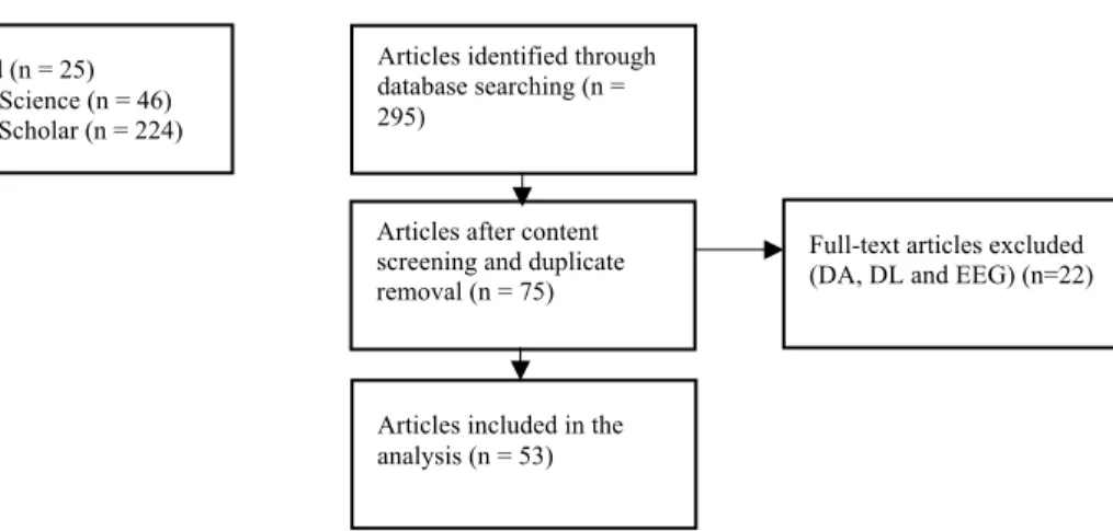
The search was conducted on 3rd January 2020 within the Google Scholar, Web of Science, and PubMed databases using the following group of keywords: (‘Data Augmentation’) AND (‘Deep Neural Network’ OR ‘Deep Learning’ OR ‘Deep Machine Learning’ OR ‘Deep Convolutional’ OR ‘Representation Learning’ OR ‘Deep Recurrent’ OR ‘Deep LSTM’) AND (‘EEG’ OR ‘Electroencephalography’). Only studies that met the inclusion criteria (Fig. 1) are included below. Further, duplicates among these databases were removed from the search results. The full texts of the remaining studies were then screened.
Inclusion criteria Exclusion criteria
• EEG classification—This review focused solely on classification based on EEG signals.
• Deep learning—In this review, DL is defined as learning using a neural network with at least one hidden layer
• EEG augmentation— This review focused on the augmentation of EEG signals.
• English Journal and conference papers, as well as electronic preprints, published were chosen as the target of this review. • Studies focusing only on EEG AND DL and DA
• Other studies, such as power analysis and feature selection with no end classification, were excluded.
6
The database queries yielded 295 matching results. Of those, 32 were duplicated. Manually screening the remaining 263 papers suggested that 188 of them were not relevant for this review (e.g., the keywords were included in the references rather than in the paper itself). We thus ended up with 75 papers, which we read carefully to make sure they meet all our inclusion criteria. We found 22 that did not meet the inclusion criteria following closer inspection (e.g., they did not focus on human subject, they did not include classification, and so on.) Hence, based on our inclusion and exclusion criteria, 53 papers were selected for inclusion in this analysis (Figure 1). The earliest one was from 2015.
Regarding our inclusion criteria, we should also mention more specifically that the DA and NN as search terms were found before 2015. For instance Image augmentation in the form of data warping can be found in LeNet-5 (1998) [37]. This was one of the first applications of CNNs on handwritten digit classification. Data augmentation has also been investigated in oversampling applications. Oversampling is a technique used to re-sample imbalanced class distributions such that the model is not overly biased towards labeling instances as the majority class
type. Oversampling was applied on EEG signal since 1970s [38] [39]. However, none of these papers meet our inclusion criteria.
2.2. Data Extraction and presentation
For each selected paper, around 40 features were extracted covering 7 categories: Origin of the article, DA types, Dataset, Task information, Preprocessing, DL strategy, Results (Table 1).
Table 1. Data items extracted for each article selected
Category Data item
Article origin Type of publication (Journal article, conference article, or in an electronic preprint repository)
Figure 1 Selection process for the papers PubMed (n = 25)
Web of Science (n = 46) Google Scholar (n = 224)
Articles identified through database searching (n = 295)
Articles after content screening and duplicate removal (n = 75)
Articles included in the analysis (n = 53)
Full-text articles excluded (DA, DL and EEG) (n=22)
7
Data augmentation (DA) DA technique used to generate new samples Parameters for DA
Magnification factor (m)
Dataset Quantity of data, subjects, classes, channels Task information Task type
Preprocessing Frequency range used for analysis EEG signal features
Deep-learning strategy Main characteristics of NN, such as number of convolutional layers, hidden layers, activation function of hidden layers and output.
Results Decoding accuracy
3. Results
3.1. Origin of the selected studies
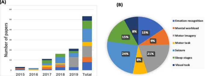
Our research methodology returned 26 journal papers,16 conference and workshop papers, and 11 preprints (arXiv or bioRxiv) that met our inclusion criteria. There were 4 papers in IEEE Transactions on Neural Systems and Rehabilitation Engineering, 3 papers in Biomedical Signal Processing and Control and the rest of the papers were each in a different journal (see Table 1 for details). Interestingly, we found no papers that fulfilled our search criteria before 2015. Further, testament to the growing importance of DA for EEG is the clear year-by-year rise in the number of papers answering our search criteria from 2015 to 2019 (Figure 2A).
3.2. EEG classification task
The EEG tasks in these papers fell into 7 groups: seizure-detection (24%), motor imagery (21%), sleep stages (15%), emotion recognition (15%), mental workload (9%), motor task (8%), and visual task (8%) (Figure 2B). The following describes these EEG tasks (see Table 6 for more details):
3.2.1. Seizure-detection studies. A seizure is a sudden, uncontrolled disturbance in the electrical activity of the brain. For seizure detection in epilepsy, EEG signals are recorded during seizure and non-seizure periods. The goal of these studies is to detect upcoming seizure and preemptive notification to the patients [40, 41]. Seizure manifestations on EEG are extremely variable both inter- and intra-patient. Naturally, non-seizure events are easy enough to record. But seizures tend to be rare. DA has been successful at increasing the number of rare events (seizures) in the dataset and thus at increasing the accuracy of seizure-detection algorithms.
3.2.2. Motor imagery tasks. These studies instruct subjects to imagine moving their limbs, tongue, or other body parts. Motor imagery EEG decoding is an important method in brain-computer interfaces (BCI) that has the potential to help highly disabled people communicate with the outside world without relying on muscle activity (e.g. [42]).
3.2.3. Sleep stages scoring tasks. Studies on sleep-stage classification record the EEG signal of subjects overnight. These signals are then scored and classified to wakefulness (W) and then 4 stages of sleep based on the American Academy of Sleep Medicine(AASM) scoring manual:
8
Rapid eye movements, or REM (R) and 3 non-REM stages (N1, N2, and N3) [43, 44]. The eventual application of this research focuses on sleep related disorders, such as sleep apnea, insomnia, and narcolepsy (e.g. [45, 46]).
Figure 2. EEG classification task. (A) Number of publications per domain of EEG task per year. (B)The percentage of different EEG classification task across all studies.
3.2.4. Emotion recognition tasks. Here subjects watch video clips, which have been categorized by experts as eliciting various emotions. Facial expressions and EEG signals are then recorded from the subjects. However, some subjects may hide their real emotions using misleading facial expressions. Therefore, EEG signals and emotion self-assessment typically follows. The result can be parsed into valence and arousal scales. Emotion recognition is a crucial problem in human-computer interaction (HCI) for example: virtual reality, video games, and educational systems (e.g. [28]).
3.2.5. Mental workload tasks. Subjects are here instructed to carry out different mental tasks of varying complexity. The results of these studies reflect the interaction between the human inner cognitive capacity and the level of task complexity. Research into mental workload has
applications in BCI performance monitoring and in cognitive stress monitoring (e.g. [47]).
3.2.6. Motor tasks. Here, subjects are instructed to either rest or move some parts of their bodies. Researchers use such tasks to design, modify or improve classification methods for different applications (e.g. [48]).3.2.7. Visual tasks. These studies focus on the detection and classification of the intentions and decisions of subjects while they watch rapidly changing sequences of pictures or letters. This helps to improved non-verbal communication systems and BCI (e.g. [49]).
3.3. Data and Reproducibility
We collected dataset information for 53 papers. This information included:
• Data quantity: Amount of data in the study (total hours of recording or number of samples) • Number of Channels: Number of channels recorded and which of them were used for analysis • Subjects: Number of recorded participants and which of them were analyzed
9
See Table 6 for more details.
3.4. Pre-processing and Feature extraction
The analysis of EEG signals is typically carried out by one of two methods. The first is event-related potentials, which are fluctuations of the potentials over time that are locked to an event (e.g., to 'stimulus onset' or 'button press'). The second is spectral analysis of rhythmic
oscillations, which reflect the synchronized activity of very large populations of neurons.
Regardless of the analysis method, it is an aggregate signal emanating from the neuronal activity of millions or more brain cells, which has been transduced through several layers of tissue, fluid, bone, etc. It also potentially includes undesired electrophysiological signals, such as
electromyograms (EMG) of muscle contractions specifically eye blinks, heart beats, and others. Therefore, the EEG signal is inherently noisy. Though various filtering and de-noising
techniques strive to decrease the noise in favor of the underlying neural activity. In the 53 studies we found, 85% (45 studies) removed the artifacts manually—mainly using high, low, and band pass filtering. Importantly, this means that 15% of the studies (8 studies) did not remove artifacts manually. Of those 8 studies, 7 did not take any action to remove artifacts, and the remaining study did not address artifact removal.
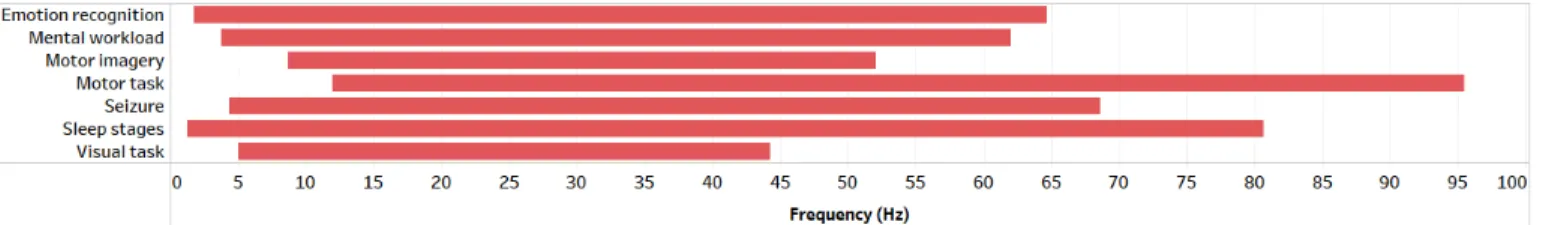
Most studies used frequency domain filters to limit the bandwidth of the EEG signals. This enabled them to focus on a certain frequency range that was of interest. Roughly, half of the reviewed papers low pass filtered the signal below low gamma band or 40 Hz. The filtered frequency ranges organized by task type (Figure 3). We found that there were no studies that specifically check the role of this filtering for NN [23].
Figure 3. Frequency range used in EEG analysis for each identified study, organized by EEG task type.
3.4.1. Input Formulation
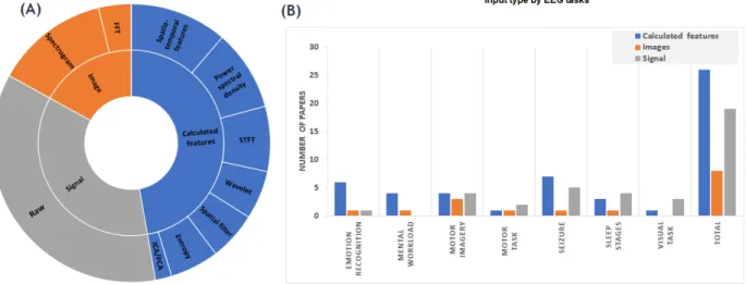
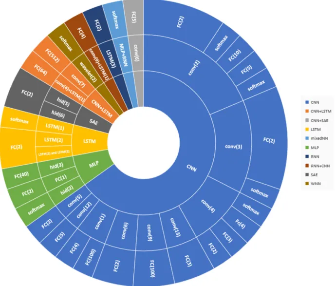
The inputs to the NNs in the studies that fulfilled our inclusion criteria, fell into three categories. The first included raw EEG signals (in the time domain) (36%). The second calculated features from the raw signals and used those as inputs (49%). And the third used spectrograms, processed as images (15%). The selection of input formulation heavily depended on the task type and deep-learning architecture. Thus, we can see that most of the studies used calculated features to train their proposed NNs. When attempting to find behavioral patterns, it is common to analyze specific frequency ranges of EEG signals. Wavelet, entropy, spatial filter, short-time Fourier transform (STFT), spatio-temporal features, and power spectral density were used in the reviewed papers to calculate the features of EEG the signals. Raw EEG values was another popular feature for training NN. It’s interesting that NNs can learn complicated features from large amount of raw data. Many NNs, especially RNN, used spectrogram and fast Fourier transform (FFT) to convert EEG signals to images (Figure 4). Hence, in general, studies run the
10
gamut from using raw EEG to heavily engineered features. When we analyzed the studies that fulfilled our inclusion criteria based on the input formulation and on the EEG task, we found that (Emotion recognition, mental workload, motor imagery, and seizure) mostly used calculated features. Motor task, sleep stages, and visual task chose signal values as their input primarily (Figure 4).
Figure 4. Input formulation across all reviewed papers. (A) The inner circle shows the general input formulation, while the outer circle shows more specific details. (B) Number of papers for general input formulation compared across different tasks.
3.5. Deep learning architectures
Deep learning is a subfield of machine learning based on artificial neural networks, which can be thought of as learn hierarchical representations of the input data through non-linear
transformations. While beginning to rise to prominence in the late 2000’s, in the few years since, it has arguably revolutionized the field, achieving remarkable accuracy on and discovering intricate structures in complex and high-dimensional data, such as image classification, speech recognition, and automated translation. Various deep learning architectures have been developed since, with this fast-moving research field routinely producing new architectures. We discerned 6 different categories in deep learning: Convolutional Neural Networks (CNN), Recurrent Neural Networks (RNN), Multi-layer perceptrons (MLP), Stacked Auto Encoders (SAE), Long Short-Term Memory (LSTM), and hybrid combinations of the above. By order of prevalence these were: CNN (62%), Hybrid (16%), MLP (8%), SAE (6%), LSTM (6%), and RNN (2%) (Figure 5).
11
Figure 5. Deep learning architecture across all studies
Figure 6 visualizes the aggregated information about DL architecture of reviewed studies. This figure helps to understanding the trends in the formation of specific deep-learning architectures. For more details seeTable 6.
12
Figure 6. Aggregated information of deep learning architectures. The inner circle shows the general DL architecture, the middle circle, shows the primary design features, such as the hidden layers or convolutional layers, and the outer circle shows the last layer of DL architecture. FC: Fully connected, hid: Hidden layers, softmax: Softmax fuction.
Figure 7, visualizes the proportion of input formulation by DL architecture. As is apparent, the specific input formulation strategies varied significantly as a function of the type of the deep learning architecture. While there was not a clear consensus for all studies together, RNN and SAE architectures used only images and calculated features as inputs, respectively. Hybrid, CNN and MLP studies included instances of all 3 information types. Interestingly MLP and CNN used directly signal values as inputs.
13
Figure 7. The percentage of input formulation by chosen DL architecture 3.6. Data Augmentation methods
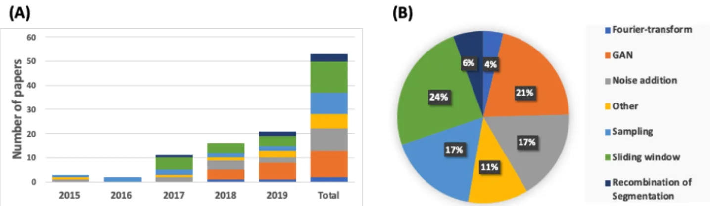
This section details the methods found for methods that have so far been used to augment EEG signal for machine learning. Data augmentation (DA) comprises the generation of new samples to augment an existing dataset by transforming the existing samples in a manner that increases the accuracy and stability of the classification or regression. Exposing the classifier to more variable representations of its training samples makes the model more invariant and robust to transformations of the type that it is likely to encounter when attempting to generalize to unseen samples. Further, increasing the size of the training set facilitates training more complex models with additional parameters and/or reducing overfitting. In recent years, DA techniques have received widespread attention and achieved appreciable performance boosts for DL on EEG signals. Here we cover all the papers that we were able to find up to and including 2019. The first paper was found in 2015. The testament to the growing importance of DA for EEG is that 37 out of 53 papers (72%) we found are from 2018 and 2019 Figure 8.
The DA for DL-based EEG in 53 papers fell into 7 categories in our analysis: noise addition (17%), GAN (21%), sliding window (24%), sampling (17%), Fourier transform (4%), recombination of segmentation (6%) and other (11%) Figure 8. Below we discuss each DA method in much more detail.
3.6.1. Noise addition
In our research, we found two main categories for adding noise to the EEG signals in purpose of DA: (1) Add various types of noise such as Gaussian, Poisson, Salt and pepper noise, etc. with different parameters (for instance: mean (!) and standard deviation (#)) to the raw signal (2)
14
Convert EEG signals to sequences of images and add noise to the images. Nine papers used noise addition method to increase training dataset.
Figure 8. DA across all studies. (A) Number of publications per domain of DA per year. (B) The percentage of different DA methods across all studies. Note that we only collected data until January 2020.
In 2015, Bashivan et al. transformed EEG signals into a sequence of topology-preserving multi-spectral (2D feature images) in a specific time interval [50]. Fast Fourier Transform (FFT) was performed on the mental load EEG signals to estimate the power spectrum of the signal in three frequency bands of theta (4-7Hz), alpha (8,13Hz), and beta (13-30Hz). A single image was constructed from spectral power within three prominent frequency band which is extracted from each electrode location. The sequences of image representations fed into the LSTM and CNN for the EEG classification. For addressing the unbalanced ratio between number of samples and number of model parameters, they randomly added various noise level to the images. However, augmenting the dataset did not improve the classification performance and even for higher value of noise, the error rate increased.
Z. Yin et al. (2017) proposed an adaptive DL model based on Stacked Denoising AutoEncoders (SDAE), which was designed for cross-session Mental Workload (MW) classification using EEG [51, 52]. They could increase the accuracy of their model by adding Gaussian white noise to the EEG feature vector (µ = 0.01, m = 2,3,4,5, 6). This vector contains centroid frequency, log-energy entropy, mean, five power components, Shannon entropy, sum of log-energy, variance, zero-crossing rate of each channel and power differences between four selected channel pairs. Their classification accuracy on an independent dataset improved from 76.5% (without DA) to 85.5% (with DA). The highest classification accuracy was achieved with m=6 and the lowest with m=0 (without DA). They concluded that the number of samples (trials) in the original dataset was insufficient for training the NN.
Wang et al. (2018) added Gaussian white noise to their training data (in the time domain) to obtain new samples for an emotion-recognition task [28]. In their experiments, EEG signals were recorded while subjects were watching emotionally loaded videos. They used differential entropy (DE) features to train their proposed classifiers. For EEG signals, the DE feature is equivalent to the logarithm of the energy spectrum in the delta (1–3 Hz), theta (4–7 Hz), alpha (8–13 Hz), beta (14–30 Hz), and gamma (31–50 Hz) frequency bands. The authors opted for Gaussian noise due to concerns that adding some local noise (i.e., noise that affects EEG data locally) such as Poisson or salt-and-pepper may change the intrinsic features of EEG signals. The experimental
15
results on SEED dataset showed that by augmenting training dataset 30 times, the accuracy of ResNet improved from 34.2% to 75%, better than LeNet (from 49.6% to 74.3%).
R. Hussein et al. (2018) used another DL technique, using a recurrent neural network (RNN) and Long Short-Term Memory (LSTM) network. Their goal was automatic detection of epileptic seizures using EEG signals [53]. And they reported that they improved the robustness of their model by adding Gaussian white noise, muscle artifacts and eye-blinking. Though they did not give any specific details about white noise they used as DA methods and the model performance wasn’t compared for DA vs. non-DA.
S. Kuanar et al. (2018) also used an LSTM with a convolutional neural network (CNN) to learn robust features and predict the levels of cognitive load from EEG recordings [47]. They
transformed the EEG time-series into a sequence of multispectral images that carried spatial information—theta (4-7Hz), alpha (8-13Hz), and beta (13-30 Hz). The data was once again augmented by adding various Gaussian noise level to the images. Though they did not give any specific details about white noise they used as DA methods and the model performance wasn’t compared for DA vs. non-DA.
E. Salama et al. (2018) generated the noisy EEG signals, by adding Gaussian noise with zero mean and unit variance to the original input EEG training dataset [54]. They set the signal-to-noise ratio (SNR) between original EEG signal and the noisy to 5. The DA phase enhanced the performance of the proposed 3D-CNN on emotion recognition dataset. For valence and arousal classification, they achieved 79.11%(without DA) and 88.49%(with DA). For 4 combinations of valence and arousal —(low valence-low arousal), (low valence-high arousal),(high valence-low arousal) and (high valence-high arousal) they obtained 79.11%(without DA) and 87.44%(with DA).
Parvan et al. (2019) doubled the number of trials of BCI competition IV dataset 2b by adding gaussian noise with zero mean and a standard deviation of 0.15 to ovoid overfitting [55]. Their proposed CNN had 4 convolution layers as well as data augmentation and resulted in a 0.07 improvemnet in the kappa coefficient [55].
Y. Li et al. (2019) emphasized the fact that increasing depth of CNN causes a higher
classification accuracy. However, doing so may aggravate the vanishing-gradient problem and substantially increase the number of trainable parameters to be tuned, and these models may tend to be overfitting easily [56]. For four-class motor imagery task, they exploit the standard
deviation of Gaussian noise in the DA affects the classification result. The optimal standard deviation is 0.001with zero mean on 2 imagery task datasets (table). It is noticeable that for almost all subjects, the performance has been significantly improved after DA. Furthermore, by comparing confusion matrix before and after DA, they showed that for a specific imagery task, DA worked well except for one task(feet). Table 2 shows all the papers used noise addition as their DA technique. From this table, we can see that there is lack of information about noise addition parameters (!: mean, #: standard deviation), magnification factor (m) and reported accuracy before and after DA. Maybe this is because that their problem wasn’t DA topic and they wanted to increase just performance accuracy.
16 Stu dy Dataset Task information Input formulat ion Deep learning strategy Noise Addition parameters Accura cy (witho ut DA) Accura cy (with DA) [50] University of Memphis Institutional review board 13 subjects 2670 trials 64 channels Mental workload 4-13 Hz Images, FFT CNN+LSTM Conv(7) + FC(512) Relu, softmax NA NA Did not improv ed [51] SDAE 8 subjects 180 min/subject 1 channel 2 class Mental workload 1.5-40Hz Calculat ed features, Power spectral density SAE Hid(5) + FC(2) Sigmoid, NA σ = 0.01, µ = 0,m = 6 NA 93% [52] AutoCAM 7 subjects 1h 11 channel Mental workload 1-40 Hz Calculat ed features, FFT and power spectral SAE Hid(6) + FC(2) Sigmoid, sigmoid σ = [0.1,0.2, … 1.5] , µ = 0, m = 6 76.5% 85.5% [28] SEED 14 subjects 1890 trials 62 channels 3 class Emotional recognition 1-50 Hz Calculat ed features, Entropy CNN Conv(4) + FC(3) sigmoid σ = 0.2, µ = 0,m = 30 49.6% 74.3% [28] SEED 14 subjects 1890 trials 62 channels 3 class Emotional recognition 1-50 Hz Calculat ed features, Entropy CNN Conv(13)+FC( 3) sigmoid σ = 0.2, µ = 0,m = 30 34.2% 75% [28] MAHNOB-HCI 30 subjects 527 trials 32 channel 3 class Emotional recognition 1-50Hz Calculat ed features, Entropy CNN Conv(13)+FC( 3) σ = 0.2, µ = 0,m = 30 40.8% 45.4%
17 [53] Bonn University 5 subject [2,3,5] class Seizure [0.53, 40] Hz Raw signal LSTM softmax Gaussian white noise+(mu scle and eye blink) NA 2 class: 99% [47] NIMHANS 22 subject, 6490 trials(8 hours) 64 channels 4 class Mental workload 4-30 Hz Calculat ed features, power spectral density RNN+CNN Conv(9)+LST M(1) Relu, softmax NA Add noise to image M: NA NA 93% [54] DEAP 32 subject 40min/subjec t 32channels 2 and 4 class Emotion recognition [1,50]U[60, end) Hz Calculat ed features Spatio-temporal CNN Conv(2) Relu, softmax 2 = 1, µ = 0, m=[10,30,50 ] 79.11 % 79.12 % 88.49 % 87.44 % [55] BCI competition IV 2b 9 subjects 5 sessions 3 channels Motor Imagery [0.5,100] Hz Raw signal CNN Conv(4)+FC(2 ) Elu, softmax σ = 0.15 , µ = 0,m = 2 NA NA [56] BCI competition IV 2a 9 subject 72trials/subje ct 22 channel 4 class Motor imagery 7-125 Hz Calculat ed features Spatio-temporal CNN Conv(1) FC(4)+softma x Relu, sigmoid 0 = 0.001, µ = 0, Report ed subject by subject e.g. 70% Increas ed 77.9% [56] High Gamma dataset(HGD ) 30 subjects 7000trials/su bject 1channel 2 class Motor imagery 7-125 Hz Calculat ed features Spatio-temporal CNN Conv(1) FC(4)+softma x Relu, sigmoid 0 = 0.001, µ = 0, NA NA
18
The term Generative Adversarial Network (GAN) was first demonstrated by Goodfellow, et al. as a new framework to learn the underlying distribution of data from two competing networks: the generator (G) and the discriminator (D). While the generator makes “fake data”, the
discriminator classifies the “fake data” as real or fake using the given label as if they were playing a minimax game [57].
During the process, the generator gets better at generating data that are similar to the real data, until the discriminator fails to distinguish real from fake data Figure 9. The minimax game of a GAN is given by:
min
! max" 7(9, :) = <#~%!"#"(#)[log 9(@)] + <(~%$(()[1 − log 9(:(C))],
where 1!"#"is the distribution of the real data and 1$ is gaussian noise. 3(5) gives a probability of an input 5 belonging to the real data, while 6(7) produces fake samples that strive to trick 3 by learning how to produce data that appears to come from the distribution of the real samples, 1!"#". The optimization process utilized the Jensen-Shannon (JS) Divergence to find the minimum of the function [57].
GANs have been widely applied for generating data in many disciplines outside neuroscience and EEG. For example, In the method that Zhang et al. (2017) proposed a GAN was used to generate images from text [58]. Bousmalis, K., et al. (2017) strives to generate rendered images that are similar to images in a dataset [59]. Antoniou et al. (2017)used a GAN to create new data from three different popular image datasets: Omniglot, EMNIST, and VGG-face [60].
Specifically for augmenting EEG signals, Zhang et al. (2018) proposed a conditional deep convolutional generative adversarial network (cDCGAN) [61]. The cDCGAN is an improved version of the GAN that uses information from the labels and adds them to the model as conditional properties:
min
! max" 7(9, :) = <#~%!"#"(#)[log 9(@|E()] + <(~%$(()F1 − log 9G:(C|E))HI,
where E( and E)is the information from the corresponding labels. The dataset contained EEG signals recorded over 3 electrodes, and composed of 7 sessions, with 40 trials per second, each lasting 9 seconds. It was collected while subjects were asked to imagine moving either left or right. A CNN was trained to classify each EEG signal as Left or Right.
19
Figure 9 Diagram of Generative Adversarial Network
The EEG signals were preprocessed before feeding them into the CNN. Only 5 out of the 9 seconds of EEG in each trial were selected for processing and only alpha (7-15 Hz) frequency components were extracted as time-frequency features. Using data generated from the cDCGAN, classification accuracy increased from 83% to 86%. The authors compare the accuracies for models trained using different proportions of artificial data. However, the largest dataset only doubles the original dataset in the experiment (i.e. m=2), while others have used larger augmentation.
Piplani et al. (2018) used a GAN to generate more EEG data to increase the robustness of a “passthought authentication system” that uses the user’s EEG signals to securely log into devices [62]. The EEG signals were collected using a device with only a single channel at a sampling rate of 500Hz. The ‘negative’ samples were collected from 30 subjects who were asked to perform a series of mental task for 5 minutes while EEG was recorded. The ‘positive’ samples were collected from one subject while the subject was doing the same mental tasks for 5 mins and free to do any tasks for another 5 minutes. The dataset that trains the selected model, XGBoost, consists of 30,000 negative samples and 40,000 positive samples. Each sample is a segment of the EEG signal. These data were augmented with 10,000 artificial EEG signals that were generated from a GAN. This increased the accuracy of the model from 90.8% to 95.0%, which is noteworthy for such high accuracies.
Zhang et al. (2018) proposed a framework called Deep Adversarial Data Augmentation (DADA) for generating new data, allowing deep network classifiers to be trained on small datasets [63]. They further investigated and compared different traditional approaches for dealing with small datasets in DL applications—such as dimensionality reduction, semi-supervised learning, transfer learning, and data augmentation. DA was widely used for image data because images can be altered easily—maintaining their content on the one hand while increasing the variance of the representation of that content by rotating, cropping, scaling or just adding noise to the
20
original dataset. However, these techniques are usually not suitable for non-image data such as EEG signals. One of the examples in this study focuses on increasing the size of an EEG dataset from a BCI competition [64]. This dataset contained 3 channels (C3, Cz, and C4) of EEG
collected from 400 trials of motor imaginary tasks. Time-frequency features were extracted from these EEG signals, which formed a 32 x 32 x 3 image for each EEG signal, which was in turn used for training a CNN classifier. Compared to the traditional GAN, DADA was able to generate more diverse artificial data because of its redesigned loss function. A traditional GAN trains the discriminator on only 2 classes. In contrast, DADA uses 2K classes for the
discriminator, K for each of the real and artificial datasets. They found that accuracy increased from 74.8%, using a traditional CNN as a benchmark, to 79.3%, using the DADA model. Hartmann et al. (2018) used a slightly modified version of the Wasserstein Generative Adversarial Network (WGAN) to generate new EEG signals [65]. Training an original GAN suffered from vanishing gradients while optimizing the JS Divergence [57]. A WGAN solved this problem by minimizing the Wasserstein distance:
KGL)*+*, L,*-.H = <#~%!"#"[9(@)] − <#~%%"&'[9(@)],
where 1%"&' is the distribution of the generator that generates fake (or artificial) samples. In addition, a gradient penalty term 8(1()) = 9 ∙ ;()~+/[=>5(0, ‖∇()3(5A)‖,− 1),] was also added
to produce a useful gradient, where 1() is the distribution of 5A that are points on a line connecting
the real and fake data. Hartmann et al. improved the model by scaling 9, allowing the parameter to adjust its impact based on different Wasserstein distances [65]:
M = −KGL)*+*, L,*-.H + max NKGL)*+*, L,*-.HO ∙ Q(L#0)
The EEG signals were collected from a simple motor task experiment, in which subjects were asked to raise their left hand or to rest. There were 438 trials in total—286 were used for training, 72 for validation, and 80 for testing. Only one channel, FCC4h, was included in this experiment. All total 438 signals were used to train the WGAN model. Unlike other studies that only used classification accuracies to compare the quality of new generated data and the original data, four other evaluation metrics were used in this study: the inception score (IS) [66], Frechest inception distance (FID) [67], Euclidean distance (ED), and sliced Wasserstein distance (SWD) [68]. After comparing the different metrics, optimizing the GAN for good IS and FID produced the best EEG data approximations [65]. This method did not use any classification algorithms to validate the accuracy, therefore it is not included in Table 3 for accuracy comparison.
A conditional version of the WGAN was used by Luo and Lu (2018) to augment EEG data. Similar to cDCGAN, WGAN also utilized the label information to infer the distribution of the real data [69]. The datasets used to test the WGAN model were SEED [70] and DEAP [71]; two popular public EEG datasets for emotion recognition. The EEG signals from the SEED dataset had 62 channels. They were collected from 15 subjects while they were watching film clips selected to induce positive, negative, or neutral emotions. For each subject, 3394 epochs were recorded. The DEAP dataset had 32 channels of EEG signals recorded from 32 subjects, with 2400 epochs each while they were watching music videos. There were 2 classification tasks for the DEAP dataset: high vs low arousal and high vs low valence. Luo and Lu tried different sizes
21
for the augmented data and found that doubling the data (m=2) provided the highest accuracy comparing to other attempts (m=0.5, 1.0, 1.5). An SVM classifier trained on the augmented dataset improved 2.97% for the SEED dataset from 83.99% to 86.96%. DA seemed to have a larger effect on the DEAP dataset. While classifying arousal, there was a 9.15% improvement in classification accuracy from 69.02% to 78.71%. For valence classification, the improvement was even larger with a 20.13% increase from 53.76% to 73.89%. The method did not specifically mention the chance level accuracy for both datasets. For the SEED dataset, since there are three classes, we are assuming that the chance level accuracy is 33.33%. For DEAP dataset, the chance level accuracy is 50% for binary classification.
In 2019, Luo et al. adopted a conditional Boundary Equilibrium GAN (cBEGAN) to generate artificial differential entropy features of EEG signals on 2 popular emotion recognition dataset (SEED, SEED V) [72]. cBEGAN used the Wasserstein distance to measure the difference between two reconstruction loss distributions. The main advantage of cBEGAN is that it can overcome the instability of conventional GAN and has very quick convergence speed. They generated 50 to 2000 artifacts samples and added them to the original training dataset. With 2000 added samples, the accuracy increases from 81.9% to 87.56% for SEED; and with 1000 samples, the accuracy increases from 54.3% to 62.8% for SEED V, respectively.
Wei et al. (2019) used WGAN with gradient penalty to increase the sample diversity in seizure detection in the CHB-MIT Scalp EEG database (with 23 subjects) [73]. Testing the performance on one patient, they used generated data from the other 22 patients involved in the training. They employed a 12-layers CNN and achieved 81% accuracy (without DA) and 84% (with DA). Chang et al. (2019) used GAN to increase the size of dataset for a 2-class emotion recognition task [74]. The generator and discriminator of the GAN consists of three hidden layers, which consists of 50, 100, and 50 nodes, respectively. The number of nodes in each layer was determined after evaluations with multiple combinations of hyper parameters that showed the highest training speeds. The generator received random values between 0 and 1 and generated virtual EEG data. The discriminator received EEG collected through experiments and virtual data and distinguished the original data from the virtual data. Once the training was complete, the EEG data generated by the generator were saved. The authors increased the number of trials from 32,000 to 92,000 and by that raised the final accuracy from 97.9% to 98.4%.
Yang et at. (2019) augmentated dataset 2b competition IV BCI using a GAN network [75]. They used CNN-LSTM to classify left and right hand motor imagery task. The average accuracy for 9 subjects was 76.4%. Unfortunately, they did not report the results without DA.
Panwar et al. (2019) proposed using a class conditioned Wasserstein Generative Adversarial Network with gradient penalty (cWGAN-GP) to generate synthetic EEG data of a single channel [76]. The study claims that the cWGAN-GP method is able to counter instability and frequency artifacts problems while training an ordinary GAN [65]. The Wasserstein distance and the gradient penalty stabilized the training process [77]. The class conditioned implementation allowed the generator and discriminator to avoid mode collapsing, which is responsible for trapping the data generated from the GAN in some specific modes [65]. The proposed
22
architecture had two fully connected layers and two convolutional layers for the generatoras well as three convolutional layers and two fully connected layers for the discriminator. The dataset that the paper used to train the cWGAN-GP was collected during the BCIT X2 Rapid Series Visual Presentation (RSVP) experiment, where subjects were asked to identify target images in an image stream presented at 5Hz [78]. The dataset contained EEG signals from 10 subjects, with 5 sessions and 1 hour of recording per session using a 256-channel BioSemi system. It had two classes, target and non-target, 967 samples each, which were pre-processed using the PREP pipeline [3]. The pipeline performed band-pass filtering from 0.1 to 55Hz, referencing, bad channel interpolation and baselining. One second of signal from each trial after image onset was extracted, down sampled to 64Hz and normalized using the mean and standard deviation from each epoch. The paper used three different methods to evaluate the performance of the data generated from the cWGAN-GP: visual inspection, log-likelihood distance from Gaussian mixture models (GMMs), and classifier performance. The visual inspection and GMM results both showed that the generated data was of high quality. In classifier performance evaluation, the synthetic data size was 3828, and it was added to the training dataset during training. The
classifier trained with the synthetic data shows an improvement of 5.18% (from 50.02% to 55.2%) on cross subject evaluation and 3.12% (from 60.8% to 64.08%) on same subject evaluation using a CNN with 3 convolutional layers.
Aznan et al. (2019) had subjects look at one of three different objects, each flickering at 10, 12, or 15 Hz (each at a different frequency). Their goal was to detect which object the subject was looking at using BCI technolgy and then direct a humanoid robot toward that object. They compared three different methods: Deep Convolutional Generative Adversarial Network (DCGAN) [79], gradient panelized Wasserstein Generative Adversarial Network (WGAN-GP) [77], and Variational Auto-encoder (VAE) [80]. They then used those methods to generate synthetic EEG data to improve the classification accuracy on their Steady State Visual Evoked Potential (SSVEP) based BCI system [81]. The SSVEP-based classifier was able to pick up the corresponding frequency from the EEG. The dataset used to train the generative models is the video-stimuli dataset [81] that contains 50 samples of EEG signals collected from offline videos played to one subject, referring to subject 1 in the NAO dataset [81]. The NAO dataset has two portions—offline and online—collected from tasks the same as in the Video-Stimuli dataset using a dry EEG device with 20 channels. The three generative models were trained only using the video-stimuli dataset, while the SSVEP classifier was tested on the NAO dataset. The generated EEG samples were used to pre-train the SSVEP classifier. The offline portion of the NAO dataset for each subject was fed into the pre-train model to fine tune for that particular subject. After the classifier was trained, the online portion of the NAO dataset was used to test the performance of the classifier. Different sizes of augmentation were empirically tested and compared. The result showed that for all three methods, a sample size of 500 resulted in the best classification accuracy. Table 3 shows the performances of different methods.
Table 3 shows all the papers used GAN as their DA technique. By reporting the magnification factor and accuracy before and after DA, we think that GAN technique is trending to use as DA technique for EEG signal.
23
Table 3. All reviewed papers that used GAN as their DA technique
Study Dataset Task
information Input formulation Deep learning strategy Best Performance Augmented Size Accuracy (without DA) Accuracy (with DA) [61] BCI competition II dataset III 1 subject 280trials 3 channels 2 class Motor Imaginary EEG 7-15 Hz Calculated features spectrogram CNN cDCGAN Doubled 83% 86% [62] 30 subject 70000 trials 1 channel 2class Mental task(EEG-Based Login Authentication) Calculated feature Power spectral GAN ,XGBoost Added 10,000 samples 90.8% 95% [63] BCI competition IV dataset 2b 1subject, 400 trials, 3 channel 2 class
Motor imagery Calculated features spectrogram GAN+CNN 10 times 77.6% 79.3% [65] 1 subject, 438 trials, 1 electrode 2 class
Motor task Calculated features-spectrogram GAN-SWD NA NA NA [69] SEED 15 subjects, 62 channels, 3394 samples per subject
Emotion recognition 1-50 Hz Calculated features spectrogram CWGAN Doubled 83.99% Arousal 69.02%, Valence 53.76% 86.96% Arousal 78.17%, Valence 73.89% [69] 32 subjects, 32 channels, 2400 trials each subject
Emotion recognition 1-50 Hz Calculated features spectrogram CWGAN Doubled NA NA [72] SEED: 9 subjects, 62 channels, 3classes, 45 videos/subject Emotion recognition 1-50 Hz Calculated features cBEGAN 2000 81.9% 87.56%
24 SEED V: 16 subjects, 62 channels, 5 classes Differential entropy 1000 54.3% 62.8% [73] 23 subjects 5085 trials more than 23 channels
Seizure Raw signal CNN NA 81% 84%
[74] 18 subjects 32000 samples 14 channels
Emotion recognition
Raw signal GAN ~triple 97.9% 98.4%
[75] 9 subjects, 32 channels, 500samples/subject Motor imagery 0.5-100 Hz Raw signal CNN+LSTM NA NA 76.4% [76] 10 subjects, 256 channels, 5 hours/subject RSVP 0.1-55 Hz Raw signal CNN 3828 NA NA [81] video stimuli dataset: 1 subject, 20 channels, 50 unique samples for each of the three class NAO dataset: 3 subjects, 20 channels 50 samples per class offline, 30 samples per class online
Steady state visual evoked 9-60 Hz
Raw signal CNN 500 NA NA
3.6.3. Sliding window or overlapping window
O’shea et al. (2017) presented a novel end-to-end architecture that learns representations from raw EEG signal by CNN for the task of neonatal seizure detection [82]. Interpretation of neonatal EEG requires highly trained healthcare professionals and it is limited to specialized units. They used overlapping window to augment 1389 seizures during 835 hours of EEG signal. Each trial split into 8s epochs with 50% overlapping to have more training sample for their proposed CNN.
25
They obtained 97.1% accuracy; however they didn’t evaluate their result without overlapping or different shift lengths.
N. Kwak et al. (2017) used CNN for the robust classification of a steady-state visual evoked potentials paradigm [49]. They recorded EEG for the brain-controlled exoskeleton under
ambulatory conditions. For generating more training samples, they used overlapping window. In their results, different shift lengths from 10 ms to 60 ms out of 2-s window were compared. They found the training samples with smaller shifts, performed much better than larger ones. The highest accuracy was 99.28% for 5-class visual evoked potential task.
For Schirrmeister et al. (2017), a key question was the impact of CNN training (e.g., training on entire trials or cropping within trials) on decoding accuracies [83]. The concept of overlapping window was pushed even further in this study: First, DA by overlapping windows share
information was used to design an additional term to the cost function, which further regularizes the model by penalizing decisions that are not the same while being close in time. Second, redundant computations due to EEG samples being in more than one window were simplified, which ensured these computations were done once, thereby speeding up training. As a result, cropped training (segments of about 2 s length) increased the accuracy to 95% for CNN on high pass filtered data (The authors did not report the accuracies before DA).
Ullah et al. used a 1D-CNN for research on epilepsy detection [84]. The number of trials collected in this study was not enough to train the CNN. And obtaining a large-enough dataset during seizure activity was not practical. At the same time, the available, small dataset resulted in overfitting. To overcome this problem, the authors proposed 2 methods for DA:
(Note that the EEG signal length in this dataset was 4097):
• Sliding window of length 512, stride 64, leading to 87.5% overlap. Each of these windowed signals was treated as an independent instance. Therefore, each trial was divided to 57 sub-signals.
• Sliding window of length 512 with stride 128, leading to overlap of 75%, leading to 29 sub-signals
The average accuracies were 96.45±0.13 and 95.40±0.35 using DA with 87.5% and 75% overlap, respectively (The authors did not report the accuracies before DA).
N Truong et al. (2018) used GAN for semi-supervised seizure prediction [85]. They generated extra samples to balance the Freiburg and CHB-MIT datasets. As a result, training sets are 10 times larger than original one by using overlapping window. The extra generated training dataset is by sliding a 30-s window along the time with different shift length. However, they didn’t report the accuracy achieved by different shifting length.
They achieved 60.91% and 72.63% accuracy (without DA) and 74.33%and 75.33% (with DA) for Freiburg hospital and CHB-MIT, respectively when training GAN on individual subjects. Majidov et al. (2019) proposed an efficient classification of Motor imagery EEG task by using CNN [86]. For DA, they used sliding window with different shifting length. However, their result lacks more details about DA.
Z. Mousavi et al. (2019) proposed a single-channel EEG-based automatic sleep stage
classification (2 to 6 classes) algorithm which processes the raw signals in order to learn features and automatically diagnose sleep stages using CNN [87]. The lack of balance between the data
26
of each class was challenging situation which caused biasedness of classification results and degraded accuracy. Therefore, they used overlapping technique to augment their dataset. The training set was 50% of the dataset included 7592 epochs (30s), however after DA, they had 24162 epochs (3s). They achieved to 93.55% accuracy for classification 6 classes of sleep stages. In addition, to evaluate the performance of the proposed DA, GAN was also implemented. However, according to their results, using GAN for the 6 sleep stages classification had achieved 72.33%, which is lower than overlapping window.
Avcu et al. (2019) developed an end-to-end CNN for seizure detection [88]. They strove to minimize the number of channels used (just 2 channels—Fp1 and Fp2) and compared that to the result with all channels. EEG data of 29 pediatric patients diognosed with a typical absence seizure were included in this study. In total, the data contained 1037 minutes of EEG with 25 minutes of seizure data distributed among 120 seizure onsets. To overcome the imbalance in the dataset, they applied different overlapping proportions according to existence or absence of seizures. Namely, while shifting with 5 seconds (no overlapping) was implemented to create interictal class, 0.075 second shifting was used for ictal class to create balanced input for the CNN. The sensitivity for 2-channel was 93.3% and for 18-channel was 95.8%. However, the result of DA was not reported in this study.
Tayeb at al. (2019) developed three deep-learning models: LSTM, CNN, and RNN for decoding motor imagery [89]. This group used shifting window with 4s length to reflect the partial time invariance of the data and overcome the problem of overfitting. This cropping strategy increased the training dataset by a factor of 25. The CNN architecture showed better performance and achieved a mean accuracy higher than 84% over all the 20 participants. However, their result lacks more details about DA.
Also, we found more papers which segmented the dataset to create more training data: Chambon et al. (2017) segmented the input data to 30s segment to create more dataset for each class of sleep stage [46]. Tsiouris et al. (2018) used LSTM for the prediction of epileptic seizure [90]. To overcome unbalance problem of rare seizure event, the EEG segment from the interictal class were split into smaller subgroups of equal size to the preictal class. Tang et al. (2017), proposed CNN for the failure prediction [91]. To avoid multiple instance learning issue for their CNN, they used segmentation window to have sufficient new training dataset. The length of each segment was found by adaptive Multi-scale sampling. Their result was improved from 70.9% (without DA) to 77.9% (with DA) on seizure dataset.
Although many studies used this method, there seems to be no consensus on the best overlapping percentage to use, e.g. the impact of using a sliding window with 10% overlap versus 90% overlap. Some studies tried different shifting length; but this issue still is not clear. For more information refer to Table 6.
27
3.6.4. Sampling
3.6.4.1. Oversampling
R. Manor et al. (2015), presented a CNN model for the use of single trial EEG classification in five category rapid serial visual tasks [92]. They used oversampling of the minor class
(bootstrapping) to balance the dataset. They mentioned that although this method caused some overfitting on the minor class, however, it provided a more balanced classification performance in their experiment.
Drouin-Picaro et al. (2016), proposed a CNN model to classify saccades from frontal EEG signals to aim cursor control without the need for a separate eye tracking device in provide brain-computer interfaces [93]. In order to have a balanced dataset, horizontal saccades were sampled from without replacement so that the number of horizontal saccades in the dataset was the same as the highest number of vertical saccade (either up or down). The other vertical direction was then augmented by sampling from it with replacement, to make the number of data points in each direction equal. Hence, the dataset contained roughly 3000 examples of each saccade direction. Supratak et al. (2017), used a CNN model, named DeepSleepNet, for automatic sleep stage scoring based on raw single-channel EEG. They extracted time-invariant features and used LSTM to learn transition rules among sleep stages automatically [94]. By duplicating the minority sleep stages in the original training set such that all sleep stages have the same number of samples they avoided overfitting.
Dong et al. (2017), proposed a Mixed NN for temporal sleep stage classification [95]. Because of the inherent imbalance in occurrence of the different sleep stages, the authors used oversampling to generate a new balance dataset which every sleep stage is equally presented.
Sors et al. (2018) used a CNN on raw single-channel EEG signal for scoring 5 class sleep stage [45]. They mentioned their dataset (SHHS) has a very imbalanced class distribution. In order to account for this, they tried cost-sensitive learning or oversampling but the overall performance using this approach did not improve.
Ruffini et al. (2019), randomly replicated subjects from the minority class to balance their classes [96]. Their proposed model helps for diagnosis derived from a few minutes of eye-close resting EEG signal collected at baseline idiopathic patients. They didn’t compare the result with and without DA.
Sun et al. (2019) scored the sleep stage automatically. This study presents a stage-classification method based on a two-stage neural network [97]. The first, feature learning stage can fuse network-trained features with traditional hand-crafted features. A second, RNN stage is fully utilized for learning temporal information between sleep epochs and obtaining classification results. Oversampling was used to solve a serious sample imbalance problem. Sadly, the result lacked more details about DA.
28
3.6.4.2. Subsampling
Thodoroff et al. (2016), evaluated the capacity of a deep NN to learn robust features of EEG to automatically detect seizures [98]. They randomly subsampled the majority samples of the dataset to re-balance the ratio between seizure and non-seizure data (from 1000/1 to 80/20) which facilitate the training. However, because seizure manifestations on EEG are extremely variable both intra- and intra-patients, a second challenge was the overlack of data for each patient (average of 8 seizure per patient). They trained the CNN by using 0.5 s window instead on 1 s. Using transfer learning, the general representation of a seizure on other patients learned first and then they trained the model to the specific patient using the weights previously learned as initialization.
Sengur et al. (2019) employed deep feature extraction for focal EEG signals [99]. The deep features were extracted from spectrogram images using the AlexNet, VGG16, VGG19, and ResNet50 CNN models. The FC6 and FC7 activation layers were used for feature extraction resulting in 4096 dimensional feature vectors. The obtained feature vectors were used as input to various k-NN classification models. Random subsampling was performed as the DA technique (no other details were provided about the parameters). See Table 6 for more details about these studies.
Note. There are various resampling strategies to solve this type of problem such as random under sampling, random oversampling and random under sampling with synthetic minority
over-sampling technique(SMOTE) [100-102]. We could find some studies which used SMOTE on EEG but they didn’t satisfy our criteria [35, 103]. Beside resampling techniques, another way to deal with imbalanced data is cost sensitive learning [104]. Resampling strategies and cost sensitive learning can significantly improve the predictive evaluation of the models [105]. 3.6.5. Fourier Transform
J. Schwabedal et al. (2018) proposed a new method for augmenting EEG signals when
attempting sleep-stage classification [106]. They focused on imbalanced dataset in transitional sleep stages, such as S1 and S3, which are rare events with respect to more stable stages such as wakefulness or Rapid Eye Movement (REM) sleep. Cost-sensitive learning [45], oversampling of the minority class [92, 94, 107], and subsampling the majority class [98, 108] are common techniques to address imbalanced classes. But the overall performance using these approaches resulted in some biases in prediction and did not improve the accuracy [1]. Therefore, they used Fourier Transform Surrogates to augment the EEG data. The complex Fourier components of a signal x- can be decomposed into amplitudes a- and phases j-:
x- = a-e./1
Under the assumptions of linearity and stationarity of the signal, they generated a new signal which is statistically independent from the original signal. This happened by randomizing the Fourier-transform phases [0, 2π] and then applying the inverse Fourier transform. The authors processed the CAPSLPDB sleep database, consisting of 101 overnight Polysomnographies (PSGs), using a CNN for 6 sleep stage classification. They then used the above method to