Lehigh University
Lehigh Preserve
Theses and Dissertations
8-1-2018
A Service System with On-Demand Agents,
Stochastic Gradient Algorithms and the SARAH
Algorithm
Lam Nguyen
Lehigh University, [email protected]
Follow this and additional works at:
https://preserve.lehigh.edu/etd
Part of the
Industrial Engineering Commons
This Dissertation is brought to you for free and open access by Lehigh Preserve. It has been accepted for inclusion in Theses and Dissertations by an authorized administrator of Lehigh Preserve. For more information, please [email protected].
Recommended Citation
Nguyen, Lam, "A Service System with On-Demand Agents, Stochastic Gradient Algorithms and the SARAH Algorithm" (2018). Theses and Dissertations. 4312.
A Service System with On-Demand Agents,
Stochastic Gradient Algorithms and the SARAH Algorithm
by
Lam Minh Nguyen
Presented to the Graduate and Research Committee of Lehigh University
in Candidacy for the Degree of Doctor of Philosophy
in
Industrial and Systems Engineering
Lehigh University August 2018
c
Copyright by Lam Minh Nguyen (2018) All Rights Reserved
Approved and recommended for acceptance as a dissertation in partial fulfillment of the requirements for the degree of Doctor of Philosophy.
Date
Dissertation Advisor
Committee Members:
Katya Scheinberg, Committee Chair
Martin Tak´aˇc
Frank E. Curtis
Acknowledgements
It would not have been possible to produce this dissertation without the help from the following people and it is a great pleasure to have the opportunity to express my gratitude. First, I would like to express my sincerest gratitude to my PhD advisor – Katya Schein-berg for her invaluable guidance during my PhD life. Thank you for all opportunities you provided for me. My current and future success would definitely not have been possible without your constant help.
This dissertation would not have been completed without the support of my previous PhD advisor – Alexander Stolyar. Thank you for everything you did for me during the first few years of my PhD. I really achieve a lot of knowledge from you.
I would especially like to thank Martin Tak´aˇc for his guidance. Thank you for being such a great advisor, mentor and friend for my PhD life.
I wish to thank Frank E. Curtis, a member of my dissertation committee, for his con-sistent support and constructive criticism for my courses and my dissertation. I also would like to thank Tam´as Terlaky for helping me during my initial study at Lehigh University and providing me useful advice. I am also grateful to Dzung Phan, Nam Nguyen, Jayant Kalagnanam, who served as mentors during my internship at IBM T. J. Watson Research Center.
In addition, I would like to thank my previous advisors Prasad Vemala, Kiran Desai, Susie Cox for helping me in doing research during my MBA and encouraging me to pursue my PhD degree, and my undergraduate advisors Vladimir I. Dmitriev and Alexander V. Il’in for their support at Lomonosov Moscow State University.
experience in my life.
Furthermore, I am extremely grateful to my parents, my sisters (Dasa and Masa), and my other relatives for their support.
Finally, my heartfelt gratitude goes out to my lovely wife Dung Nguyen and my beloved daughter Sarah Nguyen, who are always a motivation for me to step ahead and never give up. Before ending, I sincerely thank my wife for always supporting and being with me in my life. I would definitely not be able to get my today’s achievements without your love, support, and motivation. I will always be grateful.
Lam M. Nguyen
Contents
Acknowledgements iv List of Tables x List of Figures xi Abstract 1 Introduction 2I A Service System With On-demand Agents 4
1 A service system with on-demand agents 5
1.1 Introduction . . . 6
1.2 Switched Linear Systems and CQLF . . . 9
1.3 Model and Algorithm . . . 11
1.3.1 Model . . . 11
1.3.2 Algorithm . . . 12
1.4 Main Results . . . 14
1.5 Proof of Theorem 1.4.1 . . . 19
1.6 Proof of Theorem 1.4.2 . . . 24
1.7 Numerical and Simulation Experiments and Conjectures . . . 28
1.7.1 Stylized Scheme . . . 29
1.7.3 Global vs. Local Stability of Fluid Limits . . . 32
1.7.4 Summary of Conjectures, based on Numerical and Simulation Exper-iments. . . 33
1.8 Discussion and Further Work . . . 34
II Stochastic Gradient Algorithms 36 2 When Does the Stochastic Gradient Algorithm Work Well? 37 2.1 Introduction and Motivation . . . 37
2.2 Convergence Analyses of Stochastic Gradient Algorithms . . . 42
2.2.1 Useful Lemmas . . . 43
2.2.2 Convex Objectives . . . 45
2.2.3 Nonconvex Objectives . . . 52
2.3 Numerical Experiments . . . 56
2.3.1 Logistic Regression for Convex Case . . . 56
2.3.2 Neural Networks for Nonconvex Case . . . 57
2.3.3 Nonconvex Assumption Verification . . . 59
2.4 Conclusions . . . 60
3 SGD and Hogwild! 62 3.1 Introduction . . . 62
3.1.1 Contribution . . . 66
3.1.2 Organization . . . 67
3.2 New Framework for Convergence Analysis of SGD . . . 67
3.2.1 Convergence With Probability One . . . 69
3.2.2 Convergence Analysis without Convexity . . . 74
3.3 Asynchronous Stochastic Optimization aka Hogwild! . . . 76
3.3.1 Recursion . . . 77
3.3.2 Analysis . . . 79
3.4 Analysis for Algorithm 3 . . . 83
3.4.1 Recurrence and Notation . . . 83
3.4.2 Main Analysis . . . 86
3.4.3 Convergence without Convexity of Component Functions . . . 96
3.4.4 Sensitivity toτ . . . 97
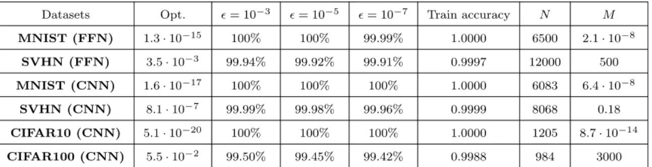
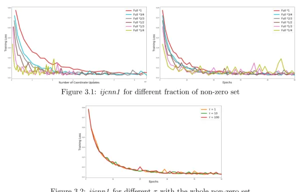
3.5 Numerical Experiments . . . 100
3.6 Conclusion . . . 102
III SARAH Algorithm 103 4 SARAH for Convex Optimization 104 4.1 Introduction . . . 104
4.2 SARAH Algorithm . . . 107
4.3 Theoretical Analysis . . . 109
4.3.1 Linearly Diminishing Step-Size in a Single Inner Loop . . . 111
4.3.2 Convergence Analysis . . . 115
4.4 A Practical Variant . . . 124
4.5 Numerical Experiments . . . 125
4.6 Conclusion . . . 128
5 SARAH for Nonconvex Optimization 130 5.1 Introduction . . . 130
5.2 SARAH Algorithm . . . 133
5.3 Convergence Analysis . . . 135
5.4 Discussions on the Mini-batches Sizes . . . 143
5.5 Numerical Experiments . . . 144
5.6 Conclusion . . . 148
6 Inexact SARAH 149 6.1 Introduction . . . 149
6.1.2 Basic Notation . . . 152
6.2 The Algorithm . . . 152
6.3 Convergence Analysis of iSARAH . . . 154
6.3.1 Basic Assumptions . . . 154
6.3.2 Existing Results . . . 156
6.3.3 Special Property of SARAH Update . . . 157
6.3.4 One-loop (iSARAH-IN) Results . . . 160
6.3.5 Multiple-loop (iSARAH) Results . . . 168
Conclusion 171
Bibliography 173
List of Tables
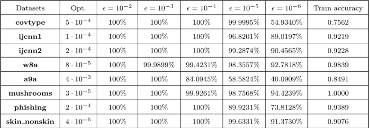
2.1 Percentage of fi with small gradient value for different threshold(Logistic
Regression) (Opt. =F(wSGD)−F(w∗)) . . . 57
2.2 Percentage of fi with small gradient value for different threshold (Neural Networks) (Opt. =k∇F(wAdam)k2) . . . 59
4.1 Comparisons between different algorithms for strongly convex functions. κ= L/µ is the condition number. . . 106
4.2 Comparisons between different algorithms for convex functions. . . 106
4.3 Summary of datasets used for experiments. . . 126
4.4 Summary of best parameters for all the algorithms on different datasets. . . 128
5.1 Comparisons between different algorithms for nonconvex functions. . . 132
5.2 Summary of statistics and best parameters of all the algorithms for the two datasets. . . 146
6.1 Comparison results (Strongly convex) . . . 151
6.2 Comparison results (General convex) . . . 152
List of Figures
1.1 An agent invitation system . . . 12
1.2 Result’s diagram . . . 17
1.3 Stylized scheme: Comparison of fluid approximations with simulations in Example 1.7.1 . . . 30
1.4 Stylized scheme: Comparison of fluid approximations with simulations in Example 1.7.2 . . . 31
1.5 Actual scheme: (X(0), Y(0), Z(0), Xtarget(0)) = (0,0,0,0) . . . 32
1.6 Actual scheme: (X(0), Y(0), Z(0), Xtarget(0)) = (0,0,0,1000) . . . 32
1.7 Problem with largeγ of the actual scheme . . . 33
1.8 A “good” value ofγ for the actual scheme . . . 33
1.9 Fluid trajectories of the systems (1.7) and (1.8) . . . 34
2.1 Stochastic Gradient Descent . . . 40
2.2 The convergence comparisons of SGD, SVRG, and L-BFGS . . . 58
2.3 The behaviors of rt . . . 60
3.1 ijcnn1 for different fraction of non-zero set . . . 101
3.2 ijcnn1 for different τ with the whole non-zero set . . . 101
3.3 covtype for different fraction of non-zero set . . . 102
3.4 covtype for different τ with the whole non-zero set . . . 102
4.1 A two-dimensional example of minwF(w) with n = 5 for SVRG (left) and SARAH (right). . . 112
4.2 An example of `2-regularized logistic regression on rcv1 training dataset for
SARAH, SVRG, SGD+ and FISTA with multiple outer iterations (left) and a single outer iteration (right). . . 112 4.3 Theoretical comparisons of learning rates (left) and convergence rates (middle
and right) withn= 1,000,000 for SVRG and SARAH in one inner loop. . . 120 4.4 An example of `2-regularized logistic regression on rcv1 (left) and news20
(right) training datasets for SARAH+ with different γs on loss residuals F(w)−F(w∗). . . 126 4.5 Comparisons of loss residuals F(w)−F(w∗) (top) and test errors (bottom)
from different modern stochastic methods oncovtype, ijcnn1, news20 andrcv1.127 4.6 Comparisons of loss residualsF(w)−F(w∗) for different inner loop sizes with
SVRG (top) and SARAH (bottom) on covtype and ijcnn1. . . 129 5.1 Algorithm SARAH . . . 133 5.2 Algorithm SARAH within a single outer loop: SARAH-IN(w0, η, b, m) . . . 134
5.3 Algorithm SARAH within a single outer loop: SARAH-IN(w0, η, b, m) . . . 145
5.4 An example of `2-regularized neural nets on MNIST and CIFAR10
Abstract
We consider a system, where a random flow of customers is served by agents invited on-demand. Each invited agent arrives into the system after a random time, and leaves it with some probability after each service completion. Customers and/or agents may be impatient. The objective is to design a real-time adaptive invitation scheme that minimizes customer and agent waiting times.
We study some aspects of the SGD method with a fixed, large learning rate and pro-pose a novel assumption of the objective function, under which this method has improved convergence rates. We also propose a convergence analysis of SGD within a diminishing learning rate regime without bounded gradient assumption in the strongly convex case.
We propose the SARAH algorithm for solving finite-sum minimization problems in the strongly convex, convex, and nonconvex cases. We also consider a general stochastic opti-mization problem by using the SARAH algorithm with inexactness.
Introduction
This dissertation contains three parts: A Service System with On-Demand Agents (Part I: Chapter 1), Stochastic Gradient Algorithms (Part II: Chapters 2 and 3), and SARAH Algorithm (Part III: Chapters 4, 5 and 6). This work appears as [55,56,52,53,51,54] .
In part I, we consider a system, where a random flow of customers is served by agents invited on-demand. Each invited agent arrives into the system after a random time, and leaves it with some probability after each service completion. Customers and/or agents may be impatient. The objective is to design a real-time adaptive invitation scheme that minimizes customer and agent waiting times. We consider a queue-length-based feedback scheme, study it in the asymptotic regime where the customer arrival rate goes to infinity; and derive a variety of sufficient conditions for the system local stability at the desired equilibrium point. Under these conditions, simulations show good overall performance of the scheme.
In part II, we study some aspects of the Stochastic Gradient Algorithm (or Stochastic Gradient Descent or SGD). In Chapter 2, we consider a standard stochastic gradient descent (SGD) method with a fixed, large step size and propose a novel assumption on the objective function, under which this method has improved convergence rates (to a neighborhood of the optimal solution set). We then empirically demonstrate that these assumptions hold for logistic regression and standard deep neural networks on classical data sets. Thus our analysis helps to explain when efficient behavior can be expected from the SGD method in training classification models and deep neural networks. In Chapter 3, we propose a convergence analysis of SGD within a diminishing learning rate regime without bounded gradient assumption in the strongly convex case, which results in more relaxed conditions
than those in [13]. We then move on the asynchronous parallel setting, and prove conver-gence of the Hogwild! algorithm in the same regime, obtaining the first converconver-gence results for this method in the case of diminished learning rate.
In part III, we propose the SARAH algorithm for solving finite-sum minimization prob-lems. We study SARAH as well as its practical variant SARAH+ for the convex case in Chapter 4. The linear convergence rate of SARAH is proven under a strong convexity as-sumption. We also prove a linear convergence rate (in the strongly convex case) for an inner loop of SARAH, a property that SVRG does not possess. In Chapter 5, we also consider a mini-batch version of SARAH for solving empirical loss minimization problems in the case of nonconvex losses. We provide a sublinear convergence rate (to stationary points) for general nonconvex functions and a linear convergence rate for gradient dominated functions, both of which have some advantages compared to other modern stochastic gradient algorithms for nonconvex losses. In Chapter 6, we consider the SARAH algorithm with inexactness. Instead of computing a full gradient at each outer iteration, we only compute a subset of samples. We also consider a general stochastic optimization problem.
Part I
A Service System With
On-demand Agents
Chapter 1
A service system with on-demand
agents
We study a system where a random flow of customers is served by servers (called agents) invited on-demand. Each invited agent arrives into the system after a random time; after each service completion, an agent returns to the system or leaves it with some fixed prob-abilities. Customers and/or agents may be impatient, that is, while waiting in queue, they leave the system at a certain rate (which may be zero). We consider the queue-length-based feedback scheme, which controls the number of pending agent invitations, depending on the customer and agent queue lengths and their changes. The basic objective is to minimize both customer and agent waiting times.
We establish the system process fluid limits in the asymptotic regime where the customer arrival rate goes to infinity. We use the machinery of switched linear systems and common quadratic Lyapunov functions to approach the stability of fluid limits at the desired equi-librium point, and derive a variety of sufficient local stability conditions. For our model, we conjecture that local stability is in fact sufficient for global stability of fluid limits; the validity of this conjecture is supported by numerical and simulation experiments. When local stability conditions do hold, simulations show good overall performance of the scheme.
1.1
Introduction
Consider a service system where a random flow of customers arrive exogenously. Servers, calledagents, can be invited on-demand at any time. Invited agents arrive into the system not immediately, but after a random delay. When a customer is matched with an agent, a service occurs. After completing the service, the agent can either leave the system or return to serve more customers. Customers and/or agents may be impatient, that is, they abandon the system if their wait in queue exceeds some random patience time. The objective is to keep waiting times of both customers and agents small. Such system is schematically shown in Figure 1.1.
The model we consider is a generalized version of that in [55, 58]. In [58], there is no abandonment for both queues, and agents always leave the system after service completions. The model in [55] also has no abandonment, but, like in our model, an agent may return to the system after a service completion. Thus, our model is more realistic in many scenarios because customer abandonment is a key factor for call center operations (see e.g. [21,80]). More specifically, the model in this chapter is as follows. Customers arrive as a Poisson process and join a customer queue if no agent is available. Agents can be invited into the system exogenously, and join an agent queue after a random exponentially distributed time. There is an infinite pool of potential agents, which can be invited to serve customers. Customer service times are i.i.d. exponential. After the service completion, the customer leaves the system while the agent can return to the agent queue with some fixed probability. The matching of customers and agents is done in first-come-first-served (FCFS) order. The head-of-the-line customer and agent are matched immediately and together go to service, that is, there cannot be non-zero number of customers and agents simultaneously in the customer and agent queues. Customers and/or agents may be impatient and the patience times are independently exponentially distributed.
The model is primarily motivated by call/contact centers (see [75]), where agents that we consider are highly skilled. It is not reasonable to set a fixed working schedule for these agents since their time is very valuable. Instead, they are invited on-demand in real time. The purpose is to design a real-time adaptive agent invitation scheme that minimizes
customer and agent waiting times. However, designing an effective, simple and robust agent invitation strategy is non-trivial due to randomness in agent behavior.
We study a feedback-based adaptive scheme of [75, 58, 55], called queue-length-based feedback scheme, which controls the number of pending agent invitations, depending on the customer and/or agent queue lengths and their changes. The algorithm analysis in this chapter is substantially more challenging due to greater generality of our model. Just like in [55,58], we consider a “stylized” version of the invitation scheme to make the analysis more tractable. Our simulation experiments in section 1.7.2 show that the behavior of the stylized scheme is very close to that of the more practical version of the queue-length-based feedback scheme.
We consider the system in the asymptotic regime where the customer arrival rate goes to infinity while the distributions of the agent response times, the service times and the patience times are fixed. We show convergence of the fluid-scaled process to the fluid limit (Theorem 1.4.1), which satisfies a system of differential equations. The key property of interest is the convergence of the fluid limit trajectories to the equilibrium point (at which the queues are zero). This property is referred to as global stability of the fluid limits. Establishing global stability appears to be very challenging, due to the fact that fluid limits have complicated behavior – there are two domains where they follow different ODEs, and a “reflecting” boundary. In this chapter, we focus on thelocal stabilityof fluid limits, defined as the stability of the dynamic system which describes fluid limit trajectories away from the boundary. Themain results in this chapter (Theorem 1.4.2) give sufficient local stability conditions; the proof uses the machinery of switched linear systems and common quadratic Lyapunov functions [39, 74]. Theorem 1.4.2 implies many useful sufficient local stability conditions (Corollaries 1.4.1 - 1.4.12) for special cases, including those where customers never abandon or agents certainly leave the system after service completions. (Some of these corollaries – namely, Corollaries 1.4.9, 1.4.10 and 1.4.12 – strengthen the results in [55] for the non-abandonment system.) These sufficient local stability conditions are robust and easy to achieve in practice. Finally, we conjecture that, for our model, local stability is in fact sufficient for global stability, based on a large number of numerical and simulation experiments. Our simulation experiments also show good overall performance
of the feedback scheme when the local stability conditions do hold.
The model has many applications, or potential applications. For a general discussion of modern call/contact centers and their management, see, e.g. [2, 45]. Another example is telemedicine [7], where “agents” are doctors, invited on-demand to serve patients remotely. The model also arises in other applications, such as crowdsourcing-based customer service (see e.g. [20,9]), taxi-service system, buyers and sellers in a trading market, and assembly systems. The model has relation to classical assemble-to-order models, where customers are orders and “invited agents” are products, which cannot be produced/assembled instantly. The model is also related to “double-ended queues” (see e.g. [29,41]) and matching systems (see e.g. [24]); although in such models arrivals of all types into the system are typically exogenous, as opposed to being controlled.
Organization. The rest of the chapter is organized as follows. Some background facts on switched linear systems and common quadratic Lyapunov functions are given in section 1.2. In section 1.3, we describe the model and algorithm in detail. Section 1.4 states the main results of the chapter, which are proved in sections 1.5 and 1.6. Section 1.7 provides numerical and simulation experiments; it also contains our conjectures about global and local stability of fluid limits, supported by these experiments. A discussion of the results and future work is in section 1.8.
Basic notation: SymbolsN,Z,R,R+denote the sets of natural, integer, real, real
non-negative numbers, respectively. Rd denotes thed-dimensional vector space. Rd×d denotes
the set of alld×dreal matrices. The standard Euclidean norm of a vectorx∈Rnis denoted
kxk. For a vector a and matrix A, we write their transposes as aT and AT, respectively. For a matrix A, we write its inverse and determinant as A−1 and det(A), respectively. We write x(·) to mean the function (or random process) (x(t), t ≥ 0). For a real-valued function x(·) : R+ → R, we use either x0(t) or (d/dt)x(t) to denote the derivative, and
for x(·) : R+ → Rd, (d/dt)x(t) = (x01(t), . . . , xd0(t)). For x ∈ R, x+ = max{x,0} and x− =−min{x,0}; and sgn(x) = 1 ifx >0, sgn(x) = 0 ifx= 0, and sgn(x) =−1 if x <0. For x, y ∈ R, we denote x∧y = min{x, y} and x∨y = max{x, y}. a ⇔ b means “a is equivalent to b”; a ⇒ b means “a implies b”. We write xr → x ∈ Rn to denote ordinary convergence inRn. For a finite set of scalar functionsfn(t),t≥0,n∈N, a pointtis called
regular if for any subsetN0⊆N, the derivatives d dtnmax∈N0 fn(t) and d dtnmin∈N0 fn(t)
exist. (To be precise, we require that each derivative is proper: both left and right derivatives exist and are equal.)
Abbreviations: u.o.c. means uniform on compact sets convergence of functions, with the argument determined by the context (usually in [0,∞)); w.p.1 means with probability 1; i.i.d. means independent identically distributed; RHS means right hand side; FSLLN means functional strong law of large numbers; CQLF means common quadratic Lyapunov function;LTI system meanslinear time-invariant system.
1.2
Switched Linear Systems and CQLF
Common quadratic Lyapunov functions for switched linear systems play an important role in deriving our results. In this section, we provide some necessary background.
Consider a switched linear system
ΣS :u0(t) =A(t)u(t) , A(t)∈ A={A1, . . . , Am} (1.1) where Ais a set of matrices in Rn×n, and t→A(t) is a mapping from nonnegative real
numbers intoA. (Usually, as in [74], this mapping is required to be piecewise constant with only finitely many discontinuities in any bounded time-interval. In our case this additional condition is not important, because our switched system will have a continuous derivative; see equation (1.8) below.) For 1≤i≤m, theith constituent system of the switched linear system (1.1) is thelinear time-invariant (LTI) system
ΣAi :u
0(t) =A
iu(t). (1.2)
The origin is anexponentially stable equilibrium of the switched linear system Σsif there exist real constantsC >0,a >0 such thatku(t)k ≤Ce−atku(0)kfort≥0, for all solutions
u(t) of the system (1.1) (see [27,74]).
A symmetric squaren×nmatrixM with real coefficients ispositive definite ifzTM z >0 for every non-zero column vector z ∈ Rn. A symmetric square n×n matrix M with real coefficients is negative definite if zTM z < 0 for every non-zero column vector z ∈ Rn. A
square matrixA is called a Hurwitz matrix (or stable matrix) if every eigenvalue of A has strictly negative real part. The following fact is the Hurwitz criterion of matrices in R3×3
(see [62]).
Proposition 1.2.1 ([62]). Let L(λ) = det(A−λI) = 0 be the characteristic equation of matrix A in R3×3:
L(λ) =a0λ3+a1λ2+a2λ+a3= 0 , a0>0. (1.3)
Matrix A is Hurwitz if and only if a1, a2, a3 are positive and a1a2 > a0a3.
The function V(u) = uTP u is a quadratic Lyapunov function (QLF) for the system ΣA:u0(t) =Au(t) if (i)P is symmetric and positive definite, and (ii)P A+ATP is negative definite. Let {A1, . . . , Am} be a collection of n×n Hurwitz matrices, with associated stable LTI systems ΣA1, . . . ,ΣAm. Then the function V(u) =u
TP u is acommon quadratic
Lyapunov function (CQLF) for these systems ifV is a QLF for each individual system (see [39,74]).
The following facts will be used in the proof of our main results (Theorem 1.4.2).
Proposition 1.2.2 ([39, 74]). The existence of a CQLF for the LTI systems is sufficient for the exponential stability of the switched linear system.
Proposition 1.2.3 ([39,74]). Let A1 andA2 be Hurwitz matrices in Rn×n, and the differ-ence A1−A2 has rank one. Then two systems u0(t) = A1u(t) and u0(t) = A2u(t) have a
CQLF if and only if the matrix product A1A2 has no negative real eigenvalues.
Proposition 1.2.4([73]). IfA−11 is non-singular, the productA1A2 has no negative
1.3
Model and Algorithm
1.3.1 Model
Our model is a generalization of that considered in [55,58]. Customers arrive according to a Poisson process of rate Λ>0, and join a customer queue waiting for an available agent and are served in the order of their arrival. There is an infinite pool of ’potential’ agents, which can be invited to serve customers. After a potential agent is invited, it becomes a ’pending’ agent; we refer to such an event as aninvitation. A pending agent ’accepts’ its invitation and becomes ’active’ agent after a random, exponentially distributed, time with mean 1/β; we refer to such an event as anacceptance. Upon acceptance events, the new active agents join the (active) agent queue. The customer and agent queues cannot be positive simultaneously: the head-of-the-line customer and agent are immediately matched, leave their queues, and together go to service. Each service time is an exponentially distributed random variable with mean 1/µ; after the service completion, the customer leaves the system, while the corresponding agent either remains active and rejoins the agent queue – this occurs with probabilityα ∈[0,1) – or leaves the system with probability 1−α. Thus, there are two ways in which agents join the queue – when an agent becomes active (upon acceptance event) and already active agents rejoining the queue after service completions. The patience times of customers and agents are independent sequences of i.i.d. exponential random variables with rate δ ≥0 and θ≥0, respectively. When its patience time expires while a customer or server wait in queue, they leave the system. (The model in [55] is a special case of ours, with δ= 0 and θ= 0; in other words, customers and agents certainly wait in their queues until they are matched. The model in [58] is a special case of ours, with δ = 0, θ= 0 and α= 0.) Figure 1.1 depicts such a system.
Let X(t) be the number of pending agents at time t. Let Y(t) =Qa(t)−Qc(t) be the difference between the agent and customer queue lengths at time t. (Note that Qa(t) = Y+(t) andQc(t) =Y−(t).) Let Z(t) be the number of customers (or agents) in service at timet. The system state at timet is (X(t), Y(t), Z(t)).
Figure 1.1: An agent invitation system
1.3.2 Algorithm
The queue-length-based feedback scheme in [55, 58, 75], referred to as the actual scheme, maintains a “target”Xtarget(t) for the number of pending agentsX(t). Xtarget(t) is changed by ∆Xtarget(t) = [−γ∆Y(t)−Y(t)∆t] at each timetwhen Y(t) changes by ∆Y(t) (+1 or
−1), whereγ >0 and >0 are the algorithm parameters and ∆tis the time duration from the previous change ofY. New agent invitations occur (i.e., the number of pending agents increases) if and only if X(t) < Xtarget(t), where X(t) is the actual number of pending agents; therefore, X(t) ≥ Xtarget(t) holds at all times. In addition, Xtarget(t) ≥ 0; i.e. if an update ofXtarget(t) makes it negative, its value is immediately reset to zero. Note that Xtarget(t) is not necessarily an integer.
Just like in [55,58], to simplify our theoretical analysis, we consider a “stylized” version of the actual scheme, referred to as thestylized scheme, which has the same basic dynamics, but keeps Xtarget(t) integer and assumes that X(t) = Xtarget(t) at all times; the latter is equivalent to assuming that not only agents can be invited instantly, but pending agents can be removed from the system at any time. Formally, the stylized scheme is defined as follows. There are six types of mutually independent, and independent of the past, events that affect the dynamics of X(t),Y(t) andZ(t) in a small time interval [t, t+dt]:
• a customer arrival with probability Λdt+o(dt),
• an acceptance with probabilityβX(t)dt+o(dt),
unlike other events, it is triggered by the algorithm itself, as opposed to other events triggered by customers’ and/or agents’ “movement” in the system,
• a service completion with probabilityµZ(t)dt+o(dt),
• an abandonment in the customer queue with probabilityδY−(t)dt+o(dt),
• an abandonment in the agent queue with probabilityθY+(t)dt+o(dt). The changes at these event times are described as follows:
• Upon a customer arrival, if Y(t) > 0, Z(t) changes by ∆Z(t) = 1; and if Y(t) ≤0, Z(t) changes by ∆Z(t) = 0. Y(t) changes by ∆Y(t) = −1, and X(t) changes by a random quantity with average γ >0. For example, if γ = 1.7 and ∆Y(t) =−1, then ∆X(t) = 2 with probability 0.7 and ∆X(t) = 1 with probability 0.3. Note that if γ is integer, ∆X(t) = γ w.p.1. To simplify the exposition, we assume that γ >0 is an integer.
• Upon an acceptance event, if Y(t)<0, Z(t) changes by ∆Z(t) = 1; and if Y(t) ≥0, Z(t) changes by ∆Z(t) = 0. Y(t) changes by ∆Y(t) = 1, and X(t) changes by ∆X(t) =−(γ∧X(t)), that is, the change is by−γ butX(t) is kept to be nonnegative.
• Upon a type-3 event, if X(t) ≥ 1, the change ∆X(t) = −sgn(Y(t)) occurs; and if X(t) = 0, the change ∆X(t) = 1 occurs if Y(t)<0 and ∆X(t) = 0 ifY(t)≥0.
• Upon a service completion, (a) if the agent returns to the agent queue (with probability α), then if Y(t) < 0, the change ∆Z(t) = 0 occurs; and if Y(t) ≥ 0, the change ∆Z(t) = −1 occurs; Y(t) changes by ∆Y(t) = 1, and ∆X(t) = −(γ∧X(t)). (b) If the agent leaves the system (with probability 1−α), thenZ(t) changes by ∆Z(t) =−1.
• Upon a customer abandonment, Y(t) changes by ∆Y(t) = 1, and X(t) changes by ∆X(t) =−(γ∧X(t)).
• Upon an agent abandonment, Y(t) changes by ∆Y(t) = −1, and X(t) changes by ∆X(t) =γ.
LetV(t) =Y+(t)+Z(t) be the total number of agents in the system at timet. Obviously, (X(t), Y(t), V(t)) is a random process with states being 3-dimensional integer vectors. How-ever, very informally, the basic dynamics of (X(t), Y(t), V(t)) under the stylized scheme can be thought of as described by the following ODE
(d/dt)X =−γ(d/dt)Y −Y
(d/dt)Y =βX−Λ +αµZ+δY−−θY+ (d/dt)V =βX−(1−α)µZ−θY+.
(1.4)
ODE (1.4) is only to provide the basic intuition for the system dynamics – it is not used in the analysis.
1.4
Main Results
We consider a sequence of systems, indexed by a scaling parameter r→ ∞. In the system with index r, the arrival rate is Λ = λr, while the parameters α, β, µ, δ, θ, , γ do not depend on r. The corresponding process is (Xr(t), Yr(t), Zr(t)), t ≥ 0. The desired system operating point, at which (Xr(t), Yr(t), Zr(t)) should be centered is given by (λr(1−
α)/β,0, λr/µ). The explanation of this choice is as follows. If an invitation scheme works as desired,Yr(t) should be close to 0; the number of customer-agent pairs Zr(t) should be close to its average value, which is λr/µ, so that the customers leave the system at rate λr; finally, Xr(t) should be close to the valueχ, such that the total average rate at which agents join the agent queue, which isχβ+ [(λr)/µ]µα, is equal to the customer arrival rate λr – this givesχ=λr(1−α)/β.
However, instead of considering process (Xr(t), Yr(t), Zr(t)), we will consider process (Xr(t),
Yr(t), Vr(t)), which is more convenient for the analysis. (Recall that Zr(t) = Vr(t)−
We define fluid-scaled process with centering as ( ¯Xr(t),Y¯r(t),V¯r(t)) =r−1 Xr(t)−λr(1−α) β , Y r(t), Vr(t)−λr µ , t≥0. (1.5)
Theorem 1.4.1. Consider a sequence of processes ( ¯Xr(·),Y¯r(·),V¯r(·)), r → ∞, with de-terministic initial states such that ( ¯Xr(0),Y¯r(0),V¯r(0))→(x(0), y(0), v(0)) for some fixed
(x(0), y(0), v(0)) ∈ R3, x(0) ≥ −λ(1−α)
β . Then, these processes can be constructed on a
common probability space, so that the following holds. W.p.1, from any subsequence of r, there exists a further subsequence such that
( ¯Xr(·),Y¯r(·),V¯r(·))→(x(·), y(·), v(·)) u.o.c. as r→ ∞ (1.6)
where (x(·), y(·), v(·))is a locally Lipschitz trajectory such that at any regular pointt≥0
x0(t) = −γy0(t)−y(t), if x(t)>−λ(1β−α) [−γy0(t)−y(t)]∨0, if x(t) =−λ(1β−α) y0(t) =βx(t) +αµ(v(t)−y+(t)) +δy−(t)−θy+(t) v0(t) =βx(t)−(1−α)µ(v(t)−y+(t))−θy+(t). (1.7)
A limit trajectory (x(·), y(·), v(·)) specified in Theorem 1.4.1 will be called a fluid limit
starting from (x(0), y(0), v(0)).
Remark 1.4.1. Equations (1.7), which a fluid limit must satisfy, are very natural. They can be thought of as rescaled centered versions of the (informal) equations (1.4). In addition, (1.7) includes a “reflection” (or, “regulation”) at the boundary x=−λ(1β−α), i.e. condition
x(t)≥ −λ(1β−α) is “enforced” as all times. This additional condition is the centered rescaled version of the condition Xr(t)≥0, which obviously must hold at all times.
Consider a dynamic system (x(t), y(t), v(t))∈R3: x0(t) =−γy0(t)−y(t) y0(t) =βx(t) +αµ(v(t)−y+(t)) +δy−(t)−θy+(t) v0(t) =βx(t)−(1−α)µ(v(t)−y+(t))−θy+(t). (1.8)
Note that the RHS of (1.8) is continuous. This dynamic system describes the dynamics of fluid limit trajectories when the state is away from the boundary x=−λ(1β−α). System (1.8) is a generalization of the system considered in [55], referred to as anon-abandonment system, which is a special case of ours withδ= 0 and θ= 0.
We say that the fluid limit is globally stable if every fluid limit trajectory converges to the equilibrium point (0,0,0); and it is locally stable if every trajectory of the dynamic system (1.8) converges to the equilibrium point (0,0,0). Note that exponential stability of the system (1.8) implies local stability.
The following theorem is the main result of this chapter. It provides sufficient exponential stability conditions for the system (1.8).
Theorem 1.4.2 (Sufficient exponential stability conditions). For any set of positive β, µ,
, γ, non-negative δ and θ, and α∈[0,1), such that either (i) γ >max ( αµ−δ β , s (2−α)µ+αδ βµ ) , (1.9) or (ii) γ >max ( αµ−δ+p(αµ−δ)2+ 4αµ2 2β , s max α(δ−µ) βµ ,0 ) (1.10)
holds, a common quadratic Lyapunov function (CQLF) of the system (1.8) exists, and the system (1.8)is exponentially stable.
In other words, conditions (1.9) and (1.10) are sufficient for local stability of our system. Theorem 1.4.2 implies the following useful sufficient local stability conditions (Corollaries 1.4.1 - 1.4.12) for special cases. Figure 1.2 depicts the connection between these results.
Figure 1.2: Result’s diagram
Corollary 1.4.1. Given all other parameters are fixed, the system (1.8) is exponentially stable for all sufficiently large γ.
Corollary 1.4.2. If αµ≤δ, then the system (1.8)is exponentially stable under condition
γ >
s
(2−α)µ+αδ
βµ . (1.11)
Corollary 1.4.3. If αµ≤δ, then the system (1.8)is exponentially stable for all sufficiently small.
Corollary 1.4.4. If αµ > δ and ≤ (2−(αµα)−µβδ+)2αδβµ , then the system (1.8) is exponentially stable under condition
γ > αµ−δ
β . (1.12)
Corollary 1.4.5. If αµ > δ and > (2−(αµα)−µβδ)+2αδβµ , then the system (1.8) is exponentially stable under condition
γ >
s
(2−α)µ+αδ
Corollary 1.4.6. If αµ≥δ, then the system (1.8)is exponentially stable under condition
γ > αµ−δ+
p
(αµ−δ)2+ 8β
2β . (1.14)
Corollary 1.4.7. If µ > δ, then the system (1.8) is exponentially stable under condition
γ > αµ−δ+
p
(αµ−δ)2+ 4αµ2
2β . (1.15)
(Note that this condition does not depend on .)
We also have the following result for the system where agents do not return to the agent queue after service completions.
Corollary 1.4.8. If α= 0, then the system (1.8)is exponentially stable for all positive β,
µ, , γ, andδ ≥0, θ≥0.
Let us consider a special case when δ = 0, referred to as acustomer non-abandonment system. Then, Corollaries 1.4.4, 1.4.5, 1.4.6, and 1.4.7 imply the following sufficient local stability conditions of the customer non-abandonment system.
Corollary 1.4.9. Ifδ = 0,α∈(0,1), and≤ (2α−2µα2)β, then the system (1.8)is exponentially stable under condition
γ > αµ
β . (1.16)
Corollary 1.4.10. If δ= 0, α ∈(0,1), and > (2α−2µα2)β, then the system (1.8)is exponen-tially stable under condition
γ >
s
(2−α)
β . (1.17)
Corollary 1.4.11. If δ = 0, and α ∈ [0,1), then the system (1.8) is exponentially stable under condition
γ > αµ+
p
α2µ2+ 8β
Note that ifθ= 0, then Corollary 1.4.11 is a simpler, equivalent version of the sufficient local stability condition in [55] for the non-abandonment system (Theorem 3 in [55]). More-over, condition (1.10) in Theorem 1.4.2 implies the following result, which does not depend on , for the non-abandonment system.
Corollary 1.4.12. If δ = 0, and α ∈ [0,1), then the system (1.8) is exponentially stable under condition
γ > (α+
√
α2+ 4α)µ
2β . (1.19)
Having a variety of these sufficient local stability conditions is useful, because some or others may be easier to verify/ensure, depending on the scenario. Note thatγandare con-trol parameters, while all other parameters are those of the system – they can be potentially measured/estimated in real time. It is not easy to give an intuitive meaning/interpretation of the above local stability conditions. Perhaps Corollary 1.4.1 is the easiest to interpret: if magnitudeγ of the system response to changes in the queue length is large enough, this is sufficient for local stability.
Remark 1.4.2. We note that our local stability results apply to more general systems, exhibiting same local behavior. For example, suppose the total number of potential agents is not infinite, by finite, scaling with r as κr, whereκ > λ(1−α)/β. Then, the fluid limits of such system satisfy the same ODE (1.8) in the vicinity of the origin, and therefore our local stability results apply as is.
1.5
Proof of Theorem 1.4.1
The proof of Theorem 1.4.1 is a generalization of the proof of Theorem 1 in [58]. However, it requires additional technical details – we present it here for completeness.
In order to prove Theorem 1.4.1, it suffices to show that w.p.1 from any subsequence of r, we can choose a further subsequence, along which a u.o.c. convergence to a fluid limit holds.
process which drives customer arrivals. N2 is the process which drives the acceptance of
invitations. N3 is the process which drives the service completions with agents leaving the
system. N4 is the process which drives the service completions with agents returning the
agent queue. N5 and N6 are the processes which drive type-3 events, when variable Yr(t)
is negative and positive, respectively. N7 is the process which drives the abandonment of
customers. N8 is the process which drives the abandonment of agents. Given the initial
state (Xr(0), Yr(0), Vr(0)), we construct the process (Xr(·), Yr(·), Vr(·)), for allr, on the same probability space via a common set of independent Poisson process [59] as follows:
Xr(t) =Gr(t) + − min 0≤s≤tG r(s) ∨0, (1.20) Gr(t) =Xr(0) +γN1(λrt)−γN2 β Z t 0 Xr(s)ds −γN4 αµ Z t 0 (Vr(s)−(Yr(s))+)ds −γN7 δ Z t 0 (Yr(s))−ds +γN8 θ Z t 0 (Yr(s))+ds + +N5 Z t 0 (Yr(s))−ds −N6 Z t 0 (Yr(s))+ds , (1.21) Yr(t) =Yr(0) +N2 β Z t 0 Xr(s)ds −N1(λrt) +N4 αµ Z t 0 (Vr(s)−(Yr(s))+)ds + +N7 δ Z t 0 (Yr(s))−ds −N8 θ Z t 0 (Yr(s))+ds , (1.22) Vr(t) =Vr(0) +N2 Z t 0 βXr(s)ds −N3 Z t 0 (1−α)µ(Vr(s)−(Yr(s))+)ds − −N8 θ Z t 0 (Yr(s))+ds . (1.23)
W.p.1, for anyr, relations (1.20)-(1.23) uniquely define the realization of (Xr(·), Yr(·), Vr(·)) via the realizations of the driving processes Ni(·). Relation (1.20), the “reflection” at zero, corresponds to the property that Xr(t) cannot become negative.
The functional strong law of large numbers (FSLLN) holds for each Poisson processNi:
Ni(rt)
r →t , r → ∞, u.o.c., w.p.1. (1.24) We consider the sequence of associated fluid-scaled processes with centering ( ¯Xr(·),Y¯r(·), ¯
r, on the same probability space as ( ¯Xr(·),Y¯r(·),V¯r(·)), let us define a modified fluid-scaled process ( ¯Xmr(·),Y¯mr(·),V¯mr(·)). Let ( ¯Xmr(·),Y¯mr(·),V¯mr(·)) start from the same initial state as ( ¯Xr(·),Y¯r(·),V¯r(·)) , i.e., ( ¯Xmr(0),Y¯mr(0),V¯mr(0)) = ( ¯Xr(0),Y¯r(0),V¯r(0)). The modified process ( ¯Xmr(·),Y¯mr(·),V¯mr(·)) follows the same path as ( ¯Xr(·),Y¯r(·),V¯r(·)) un-til the first time t, such that k( ¯Xr(t),Y¯r(t),V¯r(t))k ≥ m. Denote this time by τmr. We then freeze the process ( ¯Xmr(·),Y¯mr(·),V¯mr(·)) at the value ( ¯Xr(τmr),Y¯r(τmr),V¯r(τmr)), i.e. ( ¯Xr
m(t),Y¯mr(t),V¯mr(t)) = ( ¯Xr(τmr),Y¯r(τmr),V¯r(τmr)) for allt≥τmr.
Lemma 1.5.1. Fix (x(0), y(0), v(0)) and a finite constant m >k(x(0), y(0), v(0))k. Then, w.p.1 for any subsequence ofr, there exists a further subsequence, along which( ¯Xmr,Y¯mr,V¯mr)
converges u.o.c. to a Lipschitz continuous trajectory(xm, ym, vm), which satisfies properties (1.7)at any regular time t≥0 such that k(xm(t), ym(t), vm(t))k< m.
Proof. For the modified fluid-scaled processes ( ¯Xmr(·),Y¯mr(·),V¯mr(·)), we define the asso-ciated counting processes for upward and downward jumps. Fort≤τmr,
¯ Xmr↑(t) =r−1γN1(λrt) +r−1γN8 θr Z t 0 ( ¯Ymr(s))+ds +r−1N5 r Z t 0 ( ¯Ymr(s))−ds , (1.25) ¯ Xmr↓(t) =r−1γN2 βr Z t 0 ¯ Xmr(s) +λ(1−α) β ds + +r−1γN4 αµr Z t 0 ¯ Vmr(s) +λ µ−( ¯Y r m(s))+ ds + +r−1γN7 δr Z t 0 ( ¯Ymr(s))−ds +r−1N6 r Z t 0 ( ¯Ymr(s))+ds , (1.26) ¯ Ymr↑(t) =r−1N2 βr Z t 0 ¯ Xmr(s) +λ(1−α) β ds + +r−1N4 αµr Z t 0 ¯ Vmr(s) + λ µ −( ¯Y r m(s))+ ds + +r−1N7 δr Z t 0 ( ¯Ymr(s))−ds , (1.27) ¯ Ymr↓(t) =r−1N1(λrt) +r−1N8 θr Z t 0 ( ¯Ymr(s))+ds (1.28) ¯ Vmr↑(t) =r−1N2 βr Z t 0 ¯ Xmr(s) +λ(1−α) β ds , (1.29) ¯ Vmr↓(t) =r−1N3 (1−α)µr Z t 0 ¯ Vmr(s) +λ µ−( ¯Y r m(s))+ ds +
+r−1N8 θr Z t 0 ( ¯Ymr(s))+ds , (1.30)
and for t > τmr, all these counting processes are frozen at their values at timeτmr, that is,
¯ Xmr↑(t) = ¯Xmr↑(τmr) , X¯ r↓ m(t) = ¯Xmr↓(τmr) , ¯ Ymr↑(t) = ¯Ymr↑(τmr) , Y¯ r↓ m (t) = ¯Ymr↓(τmr) , ¯ Vmr↑(t) = ¯Vmr↑(τmr) , V¯ r↓ m(t) = ¯Vmr↓(τmr). (1.31)
Using the relations (1.20)-(1.23) and the fact that for 0 ≤ t ≤ τmr the original process ( ¯Xr,Y¯r,V¯r) and the modified process ( ¯Xmr,Y¯mr,V¯mr) coincide, we have for allt≥0,
¯ Xmr(t) = ¯Grm(t) + −λ(1−α)/β− min 0≤s≤t ¯ Grm(s) ∨0, (1.32) ¯ Grm(t) = ¯Xr(0) + ¯Xmr↑(t)−X¯mr↓(t), (1.33) ¯ Ymr(t) = ¯Yr(0) + ¯Ymr↑(t)−Y¯mr↓(t), (1.34) ¯ Vmr(t) = ¯Vr(0) + ¯Vmr↑(t)−V¯mr↓(t). (1.35) The counting processes ¯Xmr↑(·), ¯Xmr↓(·), ¯Ymr↑(·), ¯Ymr↓(·), ¯Vmr↑(·), ¯Vmr↓(·) are non-decreasing. Using FSLLN (1.24) and the fact that the processes ¯Xmr(·), ¯Ymr(·), and ¯Vmr(·) are uniformly bounded by construction, we see that w.p.1. for any subsequence ofr, there exists a further subsequence along which the set of trajectories ( ¯Xmr↑(·),X¯mr↓(·),Y¯mr↑(·),Y¯mr↓(·),V¯mr↑(·),V¯mr↓(·)) converges u.o.c. to a set of non-decreasing Lipschitz continuous functions (x↑m(·), x↓m(·), ym↑(·), ym↓(·), vm↑(·), vm↓(·)). But then the u.o.c. convergence of ( ¯Xmr(·),Y¯mr(·),V¯mr(·),G¯rm(·)) to a set of Lipschitz continuous functions (xm(·), ym(·), vm(·), gm(·)) holds, where
xm(t) =gm(t) + −λ(1−α)/β− min 0≤s≤tgm(s) ∨0, (1.36) gm(t) =x(0) +x↑m(t)−x↓m(t), (1.37) ym(t) =y(0) +ym↑(t)−y ↓ m(t), (1.38) vm(t) =v(0) +vm↑(t)−v↓m(t), (1.39)
and the following holds for t before fluid trajectory hitsk(xm(t), ym(t), vm(t))k=m x↑m(t) =γλt+γθ Z t 0 y+m(s)ds+ Z t 0 ym−(s)ds, (1.40) x↓m(t) =γβ Z t 0 xm(s) + λ(1−α) β ds+γαµ Z t 0 vm(s) + λ µ−y + m(s) ds+ +γδ Z t 0 y−m(s)ds+ Z t 0 ym+(s)ds, (1.41) y↑m(t) =β Z t 0 xm(s) + λ(1−α) β ds+αµ Z t 0 vm(s) + λ µ −y + m(s) ds+δ Z t 0 y−m(s)ds, (1.42) y↓m(t) =λt+θ Z t 0 ym+(s)ds, (1.43) v↑m(t) =β Z t 0 xm(s) + λ(1−α) β ds, (1.44) v↓m(t) = (1−α)µ Z t 0 vm(s) + λ µ−y + m(s) ds+θ Z t 0 ym+(s)ds. (1.45) Hence, x0m(t) = −γβxm(t)−γαµ(vm(t)−y+m(t)) +γθym+(t)−γδym−(t)−ym(t), ifxm(t)>−λ(1 −α) β , [−γβxm(t)−γαµ(vm(t)−ym+(t)) +γθy+m(t)−γδy−m(t)−ym(t)]∨0, ifxm(t) =−λ(1 −α) β , y0m(t) =βxm(t) +αµ(vm(t)−ym+(t)) +δy−m(t)−θy+m(t), v0m(t) =βxm(t)−(1−α)µ(vm(t)−y+m(t))−θym+(t). (1.46)
It is easy to verify that, at any regular timet≥0 such thatk(xm(t), ym(t), vm(t))k< m, properties (1.7) hold for the trajectory (xm(·), ym(·), vm(·)).
Conclusion of the proof of Theorem 1.4.1. It is easy to see that
d
From Gronwall’s inequality [19], we have
k(xm(t), ym(t), vm(t))k ≤ k(x(0), y(0), v(0))keCt for all t≥0 (1.48) For a given (x(0), y(0), v(0)), let us fix Tl >0 and choose ml >k(x(0), y(0), v(0)keCTl. For this Tl > 0, there exists a subsequence rl, along which ( ¯Xr,Y¯r,V¯r) converges uni-formly to (xml, yml, vml), which satisfies properties (1.7), at any t ∈ [0, Tl]. The limit
trajectory (xml, yml, vml) does not hit ml in [0, Tl]. Subsequence r
l = {rl
1, rl2, . . .} is such
that, w.p.1, for all sufficiently large r along the subsequence rl, ( ¯Xr(t),Y¯r(t),V¯r(t)) = ( ¯Xr ml(t), ¯ Yr ml(t), ¯ Vr ml(t)) at anyt∈[0, Tl].
We consider a sequence T1, T2, . . ., → ∞. We construct a subsequence r∗ by using
Cantor’s diagonal procedure [67] from subsequencesr1,r2,. . . (r1⊇r2 ⊇. . .) correspond-ing to T1, T2, . . ., respectively (i.e. r∗1 = r11, r2∗ = r22, . . .). Clearly, for this subsequence
r∗, w.p.1, ( ¯Xr,Y¯r,V¯r) converges u.o.c. to (x, y, v), which satisfies properties (1.7), at any regular pointt∈[0,∞).
1.6
Proof of Theorem 1.4.2
In order to prove Theorem 1.4.2, it suffices to show that LTI systems of the switched linear system (1.8) have a CQLF.
The system (1.8) is a switched linear system with m = 2. (Note that y+ =y if y ≥ 0 and y+ = 0 if y <0, andy−= 0 if y≥0 and y−=−y ify <0.) Namely, fory ≥0,
x0(t) = (−γβ)x(t) + (γαµ+γθ−)y(t) + (−γαµ)v(t) y0(t) = (β)x(t) + (−αµ−θ)y(t) + (αµ)v(t) v0(t) = (β)x(t) + ((1−α)µ−θ)y(t) + (−(1−α)µ)v(t) (1.49)
and for y <0, x0(t) = (−γβ)x(t) + (γδ−)y(t) + (−γαµ)v(t) y0(t) = (β)x(t) + (−δ)y(t) + (αµ)v(t) v0(t) = (β)x(t) + (−(1−α)µ)v(t) (1.50)
We can rewrite the systems above as two LTI systemsu0(t) =A1u(t) and u0(t) =A2u(t),
whereu(t) = (x(t), y(t), v(t))T and
A1 = −γβ γαµ+γθ− −γαµ β −αµ−θ αµ β (1−α)µ−θ −(1−α)µ , A2 = −γβ γδ− −γαµ β −δ αµ β 0 −(1−α)µ . (1.51)
Lemma 1.6.1. MatrixA1 in (1.51) is Hurwitz for all positiveβ, γ, µ,, δ≥0,θ≥0 and
α∈[0,1).
Proof. The characteristic equation of A1 is
λ3+ (βγ+µ+θ)λ2+ (β+βγµ+µθ)λ+βµ= 0. (1.52)
By Proposition 1.2.1, it suffices to verify that
βγ+µ+θ >0 , β+βγµ+µθ >0, βµ >0, and (1.53) (βγ+µ+θ)(β+βγµ+µθ)−βµ=β2γ2µ+β2γ+βγµ2+
+2βγµθ+βθ+µ2θ+µθ2 >0. (1.54)
The conditions (1.53) and (1.6) are obviously true.
Lemma 1.6.2. For positive β, γ, µ, , δ≥0, θ≥0 and α∈[0,1), matrix A2 in (1.51)is
Hurwitz if and only if
βγ+δ µ + (1−α) βγµ+δµ(1−α) β + 1 >1 (1.55)
Proof. The characteristic equation of A2 is
λ3+ (βγ+µ(1−α) +δ)λ2+ (β+βγµ+δµ(1−α))λ+βµ= 0. (1.56) By Proposition 1.2.1, it suffices to verify that
βγ+µ(1−α) +δ >0, β+βγµ+δµ(1−α)>0 , βµ >0, (1.57) and (βγ+µ(1−α) +δ)(β+βγµ+δµ(1−α))−βµ >0, which is equivalent to (1.55) since (βγ+µ(1−α) +δ)(β+βγµ+δµ(1−α))−βµ >0 ⇔(βγ+δ+µ(1−α))(βγµ+δµ(1−α) +β)> βµ ⇔ βγ+δ µ + (1−α) βγµ+δµ(1−α) β + 1 >1.
The conditions (1.57) are obviously true.
It is easy to see that Lemma 1.6.2 implies the following result.
Corollary 1.6.1. Matrix A2 in (1.51)is Hurwitz if
γ > αµ−δ
β . (1.58)
(Note that γ >0 by definition.)
Lemma 1.6.3. Matrix A2 in (1.51) is Hurwitz under the condition either (1.9)or (1.10).
Proof. This easily follows by applying Corollary 1.6.1.
Lemma 1.6.4. Matrix productA1A2has no negative eigenvalues under the condition either
(1.9)or (1.10).
non-singular and A−11 = −θ β − (α−+γθ) β α β −1 − γ 0 −1 (−γµ) µ − 1 µ . (1.59)
By Proposition 1.2.4, to demonstrate that the productA1A2has no negative eigenvalues,
it will suffice to show that [A−11+τ A2] is non-singular for allτ ≥0. We have
det[A−11+τ A2] = [β22µ2τ3+
+(β22+β2γ2µ2−2βµ2+δµ2θ+αβµ2+βδγµ2−αδµ2θ+βγµ2θ−αβδµ−αβδγµ2)τ2 +(µ2−αµ2+β2γ2−2β+δθ+βδγ+αδµ+βγθ−αµθ−αβγµ)τ + 1]/(−βµ). (1.60)
To show det[A−11+τ A2]6= 0 for all τ ≥0, it will suffice to show that the numerator of
the ratio (1.60) is strictly positive. We can represent the numerator of the ratio (1.60) as follows.
(a) Under the condition (1.9), the numerator of the ratio (1.60) is
β22µ2τ3+ (βτ −1)2+
+[(β2γ2µ2−2βµ2−αβδµ+αβµ2) +δµ2θ(1−α) +βδγµ2(1−α) +βγµ2θ]τ2+ +[µ2(1−α) +βγ(βγ−αµ+δ) +αδµ+ (βγ−αµ+δ)θ]τ (1.62)-(1.63)> 0, (1.61) since the condition (1.9) implies
γ > αµ−δ β ⇒βγ−αµ+δ >0, (1.62) and γ > s (2−α)µ+αδ βµ ⇒β 2γ2µ2−2βµ2−αβδµ+αβµ2 >0. (1.63)
Hence, the numerator of the ratio (1.60) is strictly greater than 0 under the condition (1.9).
(b) Under the condition (1.10), the numerator of the ratio (1.60) is
(βτ −1)2µ2τ+ (βτ−1)2+
+[(β2γ2µ2−αβδµ+αβµ2) +δµ2θ(1−α) +βδγµ2(1−α) +βγµ2θ]τ2+
+[(β2γ2−βγ(αµ−δ)−αµ2) +αδµ+ (βγ−αµ+δ)θ]τ (1.65)-(1.66)> 0, (1.64) since the condition (1.10) implies
γ > αµ−δ+ p (αµ−δ)2+ 4αµ2 2β > αµ−δ β ⇒β2γ2−βγ(αµ−δ)−αµ2>0 andβγ−αµ+δ >0 (1.65) and γ > s max α(δ−µ) βµ ,0 ⇒β2γ2µ2−αβδµ+αβµ2 >0. (1.66) Hence, the numerator of the ratio (1.60) is strictly greater than 0 under the condition (1.10).
Therefore, A1A2 has no negative eigenvalues under the condition either (1.9) or (1.10).
Conclusion of the proof of Theorem 1.4.2. By Lemma 1.6.1,A1 is Hurwitz for all positive
β,γ,µ,;δ≥0,θ≥0; andα ∈[0,1). By Lemma 1.6.3,A2 is Hurwitz under the condition
either (1.9) or (1.10). It is easy to verify that the difference A1−A2 has rank one. By
Lemma 1.6.4, A1A2 has no negative real eigenvalues under the condition either (1.9) or
(1.10). Hence, by Proposition 1.2.3, two LTI systems u0(t) = A1u(t) and u0(t) = A2u(t)
have a CQLF. Therefore, the system (1.8) is exponentially stable under the condition either (1.9) or (1.10).
1.7
Numerical and Simulation Experiments and Conjectures
In this section, we present some numerical and simulation experiments. These results are for both stylized and actual schemes, and all results are for the true system which includes boundary X≥0. We also put forward some conjectures based on these experiments.
λr. On the plots labeled ’fluid’, X(t), Y(y), V(t) are replaced by theirfluid approximations
X(t) =rx(t) + λr(1−α)
β , Y(t) =ry(t), V(t) =rv(t) + λr
µ ,
respectively, where (x(·), y(·), v(·) is the corresponding fluid limit.
1.7.1 Stylized Scheme
Example 1.7.1. Consider the following set of parameters, which satisfies condition (1.9):
Λ = 2000 , α= 0.5 , β = 3 , µ= 2 , γ= 1 , = 1.5 , δ= 1 , θ= 0.1
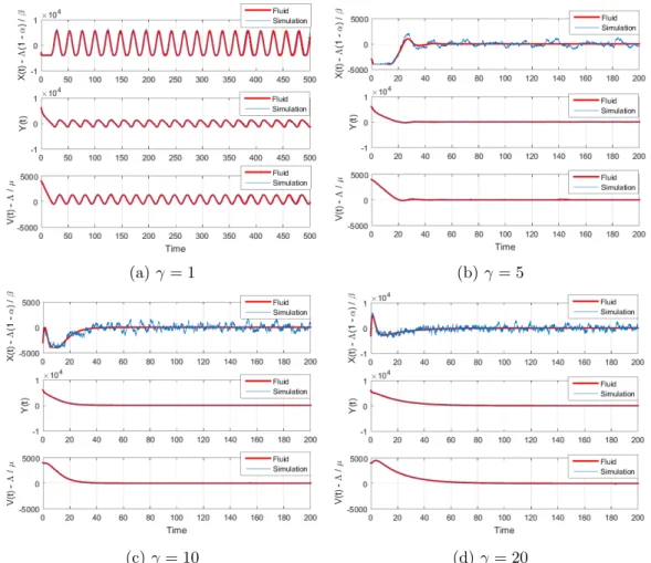
with four initial conditions: (a) (X(0), Y(0), Z(0)) = (0,0,0); (b) (X(0), Y(0), Z(0)) = (0,2000,0); (c) (X(0), Y(0), Z(0)) = (2000,−2000,1000); (d) (X(0), Y(0), Z(0)) = (2000, 4000,1000). The red line of the figure is the fluid approximation and the blue one is the simulation experiment. We see the converging trajectories on the Figure 1.3. Note that Figures 1.3b and 1.3d show that the trajectory hits the boundary on X. We also did the numerical/simulation experiments with many different sets of parameters satisfying the condition (1.9). All results, including those not shown on Figure 1.3, suggest the global stability of the system.
Example 1.7.2. We use sets of parameters:
Λ = 2000 , α= 0.9 , β = 0.05 , µ= 0.5 , = 1 , δ= 0.01 , θ= 0.01
with four different values ofγ (γ1 = 1, γ2= 5, γ3 = 10, and γ4 = 20) (Figure 1.4). The
sets of parameters with γ1 = 1 andγ2 = 5 do not satisfy the condition (1.9) while the sets
of parameters withγ3 = 10 andγ4 = 20 satisfy the condition (1.9). We consider an initial
condition (X(0), Y(0), Z(0)) = (1000,6000,2000). On the Figures 1.4b, 1.4c and 1.4d, we see that the trajectories converge. However, Figure 1.4a shows the trajectory that never converges under the set of parameters withγ1= 1.
With many numerical/simulation experiments, the results, including those not shown on Figure 1.4, suggest both local and global stability of the system for all sufficiently large γ.
(a) (X(0), Y(0), Z(0)) = (0,0,0) (b) (X(0), Y(0), Z(0)) = (0,2000,0)
(c) (X(0), Y(0), Z(0)) = (2000,−2000,1000) (d) (X(0), Y(0), Z(0)) = (2000,4000,1000) Figure 1.3: Stylized scheme: Comparison of fluid approximations with simulations in Example 1.7.1
Our simulation experiments show that the fluid trajectory provides a very good approx-imation for the behavior of stylized scheme.
1.7.2 Actual Scheme
Example 1.7.3. We conduct a simulation experiment for the actual scheme with the same set of parameters as in Example 1.7.1:
Λ = 2000 , α= 0.5 , β = 3 , µ= 2 , γ= 1 , = 1.5 , δ= 1 , θ= 0.1
with two initial conditions (X(0), Y(0), Z(0), Xtarget(0)) = (0,0,0,0) and (X(0), Y(0), Z(0), Xtarget(0)) = (0,0,0,1000). (Note that this set of parameters satisfies the condition (1.9).) The results are shown in Figures 1.5 and 1.6. We see that the magnitude of the difference betweenXtarget and the actual number of invited agentsX is very small (except
(a) γ= 1 (b)γ= 5
(c)γ= 10 (d)γ= 20
Figure 1.4: Stylized scheme: Comparison of fluid approximations with simulations in Example 1.7.2
at time 0) and can be negligible compared to their values. This explains why the trajectories of Xtarget and X are well approximated by the fluid trajectory, obtained for the stylized scheme.
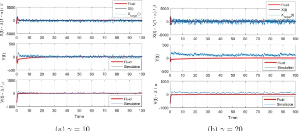
For the stylized scheme, the results suggest the global stability of our system for all sufficiently largeγ. However, the problem with large γ is that the behavior of the stylized scheme may significantly deviate from the behavior of the actual scheme, as illustrated by the following example.
Example 1.7.4. Consider the following set of parameters:
Λ = 2000 , α= 0.7 , β = 0.5 , µ= 3 , = 1 , δ = 1 , θ= 2
with two values of γ (γ1 = 10, γ2 = 20); and an initial condition (X(0), Y(0), Z(0),
(a) Fluid vs. X(t) andXtarget(t) (b)X(t)−Xtarget(t) Figure 1.5: Actual scheme: (X(0), Y(0), Z(0), Xtarget(0)) = (0,0,0,0)
(a) Fluid vs. X(t) andXtarget(t) (b)X(t)−Xtarget(t) Figure 1.6: Actual scheme: (X(0), Y(0), Z(0), Xtarget(0)) = (0,0,0,1000)
scheme deviates substantially from the behavior of the fluid trajectory with largeγ. Sinceαµ > δand≤ (2−(αµα)−µβδ)+2αδβµ , then we chooseγ= 2.3 such thatγ > αµβ−δ (Corollary 1.4.4). We can see that, with a “good” value ofγ, the behavior of the actual scheme deviates negligibly from the behavior of the fluid trajectory (Figure 1.8a) and the difference between Xtarget and X is not large compared to their values (Figure 1.8b).
1.7.3 Global vs. Local Stability of Fluid Limits
In this chapter, we have derived some sufficient local stability conditions for the fluid limits. Based on a variety of simulation experiments above for the stylized scheme, we conjecture that local stability is sufficient for global stability of fluid limits for our model. In the next example, we compare the behavior of fluid limits for the system without boundary (given by (1.8)) with that of the system with boundary (given by (1.7)).
(a)γ= 10 (b)γ= 20 Figure 1.7: Problem with largeγ of the actual scheme
(a)γ= 2.3 (b)X(t)−Xtarget(t)
Figure 1.8: A “good” value of γfor the actual scheme
Example 1.7.5. Consider two set of parameters, which satisfy the local stability conditions, so that the trajectory of the system (1.8) converges to the equilibrium point(0,0,0)(Figure 1.9). The red line of the figure is the trajectory of the system (1.7), which may hit the boundary X= 0, and the black one is the trajectory of the system (1.8), for which there is no boundary.
With many experiments, the results, including those not shown in Figure 1.9, further suggest the global stability of the fluid limits, when the local stability holds.
1.7.4 Summary of Conjectures, based on Numerical and Simulation
Ex-periments.
(a) Set 1 (b) Set 2 Figure 1.9: Fluid trajectories of the systems (1.7) and (1.8)
Conjecture 1.7.2. Given all other parameters are fixed, our system is globally stable for all sufficiently large γ.
Obviously, Conjecture 1.7.1 is stronger than Conjecture 1.7.2 because we have proved the local stability when γ is large in this chapter. We note again, however, that in a practical application the value of γ should not be made too large, because the stylized scheme behavior, which we studied in this chapter, may substantially deviate from the behavior of the actual scheme, where uninviting pending agents are not allowed.
1.8
Discussion and Further Work
In this chapter, we study a feedback-based agent invitation scheme for a model with ran-domly behaving agents and possible abandonment of customers and agents. This model is motivated by a variety of existing and emerging applications. The focus of the chapter is on the stability properties of the system fluid limits, arising as asymptotic limits of the sys-tem process, when the syssys-tem scale (customer arrival rate) grows to infinity. The dynamic system, describing the behavior of fluid limit trajectories has a very complex structure – it is a switched linear system, which in addition has a reflecting boundary. We derived some sufficient local stability conditions, using the machinery of switched linear systems and common quadratic Lyapunov functions. Our simulation and numerical experiments show good overall performance of the feedback scheme, when the local stability conditions hold. They also suggest that, for our model, the local stability is in fact sufficient for the global
stability of fluid limits. Verifying these conjectures, as well as expanding the sufficient local stability conditions, is an interesting subject for future research. Further generalizations of the agent invitation model are also of interest from both theoretical and practical points of view.
Part II
Chapter 2
When Does the Stochastic
Gradient Algorithm Work Well?
In this chapter, we consider a general stochastic optimization problem which is often at the core of supervised learning, such as deep learning and linear classification. We con-sider a standard stochastic gradient descent (SGD) method with a fixed, large step size and propose a novel assumption on the objective function, under which this method has improved convergence rates (to a neighborhood of the optimal solutions). We then empir-ically demonstrate that these assumptions hold for logistic regression and standard deep neural networks on classical data sets. Thus our analysis helps to explain when efficient behavior can be expected from the SGD method in training classification models and deep neural networks.
2.1
Introduction and Motivation
In this chapter, we are interested in analyzing the behavior of the stochastic gradient al-gorithm when solving empirical and expected risk minimization problems. For the sake of generality we consider the following stochastic optimization problem
min
whereξ is a random variable obeying some distribution.
In the case of empirical risk minimization with a training set {(xi, yi)}ni=1,ξi is a real-ization of a random variable that is defined by the i-th element of the training set. Then, by defining fi(w) :=f(w;ξi) we write the empirical risk minimization as follows:
min w∈Rd ( F(w) = 1 n n X i=1 fi(w) ) . (2.2)
More generally ξ can be a random variable defined by a random subset of samples
{(xi, yi)}i∈I drawn from the training set, in which case formulation (2.1) still applies to the empirical risk minimization. On the other hand, ifξ represents a sample or a set of samples drawn from the data distribution, then (2.1) represents the expected risk minimization.
Stochastic gradient descent (SGD), originally introduced in [66], has become the method of choice for solving not only (2.1) but also (2.2) whenn is large. Theoretical justification for using SGD for machine learning problems is given, for example, in [12], where it is shown that, at least for convex problem, SGD is an optimal method for minimizing expected risk, which is the ultimate goal of learning. From the practical perspective SGD is often preferred to the standard gradient descent (GD) method simply because GD requires computation of a full gradient on each iteration, which, for example, in the case of deep neural networks (DNN), requires applying backpropagation for all nsamples, which can be prohibitive.
Consequently, due to its simplicity in implementation and efficiency in dealing with large scale datasets, SGD has become by far the most common method for training deep neural networks and other large scale ML models. However, it is well known that SGD can be slow and unreliable in some practical applications as its behavior is strongly dependent on the chosen stepsize and on the variance of the stochastic gradients. While the method may provide fast initial improvement, it may slow down drastically after a few epochs and can even fail to move close enough to a solution for a fixed learning rate. To overcome this oscillatory behavior, several variants of SGD have been recently proposed. For example, methods such as AdaGrad [18], RMSProp [78], and Adam [30] adaptively select the stepsize for each component of w. Other techniques include diminishing stepsize scheme [13] and variance reduction methods [68,16, 28, 51]. These latter methods reduce the variance of
the stochastic gradient estimates, by either computing a full gradient after a certain number of iterations or by storing the past gradients, both of which can be expensive. Moreover, these methods only apply to the finite sum problem (2.2) but not the general problem (2.1). On the other hand these methods enjoy faster convergence rates than that of SGD. For example, when F(w) is strongly convex, convergence rates of the variance reduction methods (as well as that of GD itself) are linear, while for SGD it is only sublinear. While GD has to compute the entire gradient on every iteration, which makes it more expensive than the variance reduction methods, its convergence analysis allows for a much larger fixed stepsizes than those allowed in the variance reduction methods. In this chapter we are particularly interested in addressing an observation: a simple SGD with a fixed, reasonably large, step size can have a fast convergence rate to some neighborhood of the optimal solutions, without resorting to additional procedures for variance reduction.
Let us consider an example of recovering a signal ˆw ∈ R2 from n noisy observations
yi = yiclean +ei where yiclean = (aTiw)ˆ 2. Here, ai’s are random vectors and ei’s are noise components. To recover ˆwfrom the observation vectory, we solve a non-convex fourth-order polynomial minimization problem
min w ( F(w) = 1 n n X i=1 (yi−(aTiw)2)2 ) .
Note that there are at least two global solutions to this problem, which we denote w∗ and
−w∗. We consider two possible scenarios:
(i) All of the component functionsfi(w) = (yi−(aTiw)2)2 have relatively small gradients at both of the optimal solutionsw∗ and−w∗ of the aggregateF(w). In this case this means thatw∗ recovers a good fit for the observationsy.
(ii) There aremany indices isuch that at the optimal solutions of F(w), the associated gradients ∇fi are large. This happens when w∗ does not provide a good fit, which can happen when the noise ei is large.
We setn= 100 and generate these two scenarios by setting all the noise componentseito be small (1% of the energy ofyclean) for case (i) or setting only first 40 noise components to