ESSAYS ON THE EFFECTS OF OIL PRICE SHOCKS ON EXCHANGE RATES AND THE ECONOMY OF SAUDI ARABIA
by
MOAYAD HUSSAIN AL RASASI
B.S., King Saud University, Riyadh, Saudi Arabia, 2005 M.A., The University of Kansas, Lawrence, USA, 2009
AN ABSTRACT OF A DISSERTATION
submitted in partial fulfillment of the requirements for the degree
DOCTOR OF PHILOSOPHY
Department of Economics College of Arts and Sciences
KANSAS STATE UNIVERSITY Manhattan, Kansas
Abstract
This dissertation consists of three essays examining the consequences of oil price shocks on exchange rates and the economy of Saudi Arabia.
In the first essay, we examine the impact of oil prices on the US dollar (USD) exchange rate in the flexible monetary model framework. We find evidence, based on the impulse response function analysis from the VEC model, suggesting the negative association between oil prices and the USD against 12 currencies. Furthermore, the results from out-of-sample forecasts indicate that oil prices play an essential role in improving the forecasting power of the monetary model of exchange rate determination.
In the second essay, we analyze how G7 real exchange rates and monetary policy respond to oil supply, aggregate demand, and oil-specific demand shocks initiated by Killian (2009). Our evidence confirms that aggregate demand and oil specific demand shocks are associated with the depreciation of the real exchange rate for five countries whereas oil supply shocks lead to the depreciation of real exchange rate in four countries. Likewise, we find the monetary policy responds significantly only to aggregate demand and oil specific demand shocks in three countries while the monetary policy responds to real exchange rate shocks in four countries.
In the third essay, we investigate the differential effects of oil shocks, developed by Killian (2009), on industrial production, inflation, and the nominal exchange rate of Saudi Arabia. The reported evidence shows that industrial production responds positively only to oil supply shocks. Likewise, we find evidence indicating that there is a positive impact of aggregate demand shocks on inflation. On the other hand, we find evidence suggesting that oil supply and demand shocks are associated with the nominal exchange rate depreciation.
ESSAYS ON THE EFFECTS OF OIL PRICE SHOCKS ON EXCHANGE RATES AND THE ECONOMY OF SAUDI ARABIA
by
MOAYAD HUSSAIN AL RASASI
B.S., King Saud University, Riyadh, Saudi Arabia, 2005 M.A., The University of Kansas, Lawrence, USA, 2009
A DISSERTATION
submitted in partial fulfillment of the requirements for the degree
DOCTOR OF PHILOSOPHY
Department of Economics College of Arts and Sciences
KANSAS STATE UNIVERSITY Manhattan, Kansas
2016
Approved by: Major Professor Dr. Lance J. Bachmeier
Copyright
MOAYAD HUSSAIN AL RASASI 2016
Abstract
This dissertation consists of three essays examining the consequences of oil price shocks on exchange rates and the economy of Saudi Arabia.
In the first essay, we examine the impact of oil prices on the US dollar (USD) exchange rate in the flexible monetary model framework. We find evidence, based on the impulse response function analysis from the VEC model, suggesting the negative association between oil prices and the USD against 12 currencies. Furthermore, the results from out-of-sample forecasts indicate that oil prices play an essential role in improving the forecasting power of the monetary model of exchange rate determination.
In the second essay, we analyze how G7 real exchange rates and monetary policy respond to oil supply, aggregate demand, and oil-specific demand shocks initiated by Killian (2009). Our evidence confirms that aggregate demand and oil specific demand shocks are associated with the depreciation of the real exchange rate for five countries whereas oil supply shocks lead to the depreciation of real exchange rate in four countries. Likewise, we find the monetary policy responds significantly only to aggregate demand and oil specific demand shocks in three countries while the monetary policy responds to real exchange rate shocks in four countries.
In the third essay, we investigate the differential effects of oil shocks, developed by Killian (2009), on industrial production, inflation, and the nominal exchange rate of Saudi Arabia. The reported evidence shows that industrial production responds positively only to oil supply shocks. Likewise, we find evidence indicating that there is a positive impact of aggregate demand shocks on inflation. On the other hand, we find evidence suggesting that oil supply and demand shocks are associated with the nominal exchange rate depreciation.
Table of Contents
List of Figures ... viii
List of Tables ... x
Acknowledgements ... xiii
Dedication ... xiv
Chapter 1 - Oil Prices and the US Dollar Exchange Rate: Evidence from the Monetary Model ... 1
1.1 Introduction ... 1
1.2 The Monetary Model of Exchange Rates ... 3
1.3 Literature Review ... 6
1.4 Data ... 8
1.5 Empirical Methodology and Results ... 9
1.5.1 Preliminary Investigation ... 9
1.5.2 The Vector Error Correction Model... 18
1.5.3 Impulse Response Function Results ... 22
1.5.4 Forecast Error Variance Decomposition Analysis ... 29
1.5.5 Out of Sample Forecasts ... 32
1.6 Conclusion ... 35
Chapter 2 - Oil Price Shocks and G7 Real Exchange Rates: The Role of Monetary Policy ... 37
2.1 Introduction ... 37
2.2 Theoretical Model ... 42
2.3 Literature Review ... 45
2.4 Data ... 47
2.5 Empirical Methodology and Results ... 48
2.5.1 Unit Root Tests ... 48
2.5.2 The Vector Autoregressive (VAR) Model ... 50
2.5.3 Impulse Response Function Analysis ... 55
2.5.4 Structural Break Tests ... 61
2.5.5 The Role of Energy Intensity ... 66
2.5.6 Forecast Error Variance Decomposition ... 69
2.7 Implications For Monetary Policy ... 79
2.8 Robustness Check ... 80
2.9 Conclusion ... 81
Chapter 3 - The Effects of Oil Shocks on the Economy of Saudi Arabia ... 83
3.1 Introduction ... 83
3.2 Data ... 85
3.3 Empirical Methodology ... 86
3.3.1 Unit Root Tests ... 86
3.3.2 The Structural Vector Autoregressive (SVAR) Model ... 86
3.4 Empirical Findings ... 90
3.5 Conclusion ... 92
References ... 94
List of Figures
Figure 1.1 The Response of the USD Exchange Rate to Oil Price Shocks ... 25
Figure 1.2 The Response of the USD Exchange Rate to Relative Output Shocks ... 26
Figure 1.3 The Response of the USD Exchange Rate to Relative Money Supply Shocks ... 27
Figure 1.4 The Response of the USD Exchange Rate to Exchange Rate Shocks ... 28
Figure 2.1 Oil Prices and G7 Real Exchange Rates Movements (I) ... 38
Figure 2.2 Oil Prices and G7 Real Exchange Rates Movements (II) ... 39
Figure 2.3 The Identified Structural Shocks to Crude Oil Market ... 54
Figure 2.4 The Responses of Canadian and French Real Exchange Rates to Structural Oil Shocks ... 57
Figure 2.5 The Responses of German and Italian Real Exchange Rates to Structural Oil Shocks ... 58
Figure 2.6 The Responses of Japanese and British Real Exchange Rates to Structural Oil Shocks ... 59
Figure 2.7 The Responses of US Real Exchange Rates to Structural Oil Shocks ... 60
Figure 2.8 The Responses of British Real Exchange Rates to Structural Oil Shocks ... 65
Figure 2.9 The Responses of Real Exchange Rates to Structural Oil Shocks ... 68
Figure 2.10 The Evolution of Real Exchange Rates Shocks ... 73
Figure 2.11 The Evolution of Real Exchange Rates Shocks ... 74
Figure 3.1 Structural Shocks Decomposition ... 89
Figure 3.2 Impulse Responses of Macro Variables to Structural Oil Shocks. ... 92
Figure A.1 The Responses of Canadian and French Real Exchange Rates to Structural Oil Shocks ... 126
Figure A.2 The Responses of German and Italy Real Exchange Rates to Structural Oil Shocks ... 127
Figure A.3 The Responses of Japanese and British Real Exchange Rates to Structural Oil Shocks ... 128
Figure A.4 The Responses of US Real Exchange Rates to Structural Oil Shocks ... 129
Figure A.5 The Responses of British Real Exchange Rates to Structural Oil Shocks ... 131
Figure A.7 The Responses of Canadian and French Real Exchange Rates to Structural Oil
Shocks ... 135 Figure A.8 The Responses of German and Italian Real Exchange Rates to Structural Oil Shocks
... 136 Figure A.9 The Responses of Japanese and British Real Exchange Rates to Structural Oil Shocks
... 137 Figure A.10 The Responses of the US Real Exchange Rates to Structural Oil Shocks ... 138 Figure A.11 The Responses of the US Real Exchange Rates to Structural Oil Shocks ... 140
List of Tables
Table 1.1 Augmented Dickey Fuller (1979) Unit Root Test. ... 11
Table 1.2 Augmented Dickey Fuller (1979) Unit Root Test. ... 12
Table 1.3 Augmented Dickey Fuller (1979) Unit Root Test. ... 13
Table 1.4 Phillips and Perron (1981) and Kwiatkowski et al (1992) Unit Root Test. ... 14
Table 1.5 Phillips and Perron (1981) and Kwiatkowski et al (1992) Unit Root Test. ... 15
Table 1.6 Phillips and Perron (1981) and Kwiatkowski et al (1992) Unit Root Test. ... 16
Table 1.7 Johansen and Juselius (1990) Cointegration Test. ... 17
Table 1.8 Structural Break Tests. ... 18
Table 1.9 Forecast Error Variance Decomposition. ... 31
Table 1.10 Forecasting Accuracy Measures. ... 35
Table 2.1 Augmented Dickey Fuller (1979) Unit Root Test. ... 49
Table 2.2 Phillips and Perron (1981) and Kwiatkowski et al. (1992) Unit Root Test. ... 50
Table 2.3 T he Effect of one standard deviation Shock. ... 61
Table 2.4 Structural Break Tests. ... 63
Table 2.5 Structural Break Tests for the UK. ... 63
Table 2.6 Forecast Variance Decomposition. ... 72
Table 2.7 Forecast Variance Decomposition for the UK. ... 72
Table 2.8 Monetary Policy Responses to Structural Shocks. ... 77
Table 2.9 British Monetary Policy Responses. ... 78
Table 3.1 Augmented Dickey Fuller (1979) Test. ... 87
Table 3.2 Phillips and Perron (1981) Test ... 87
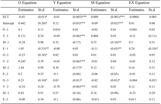
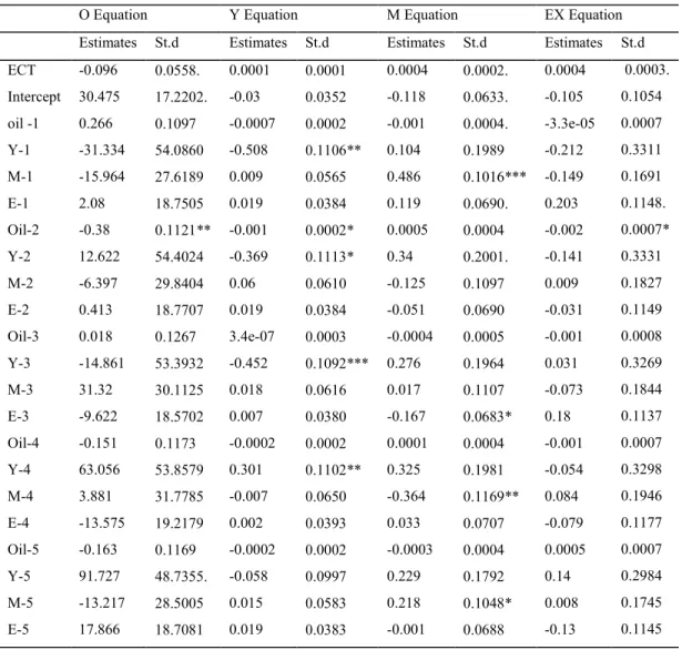
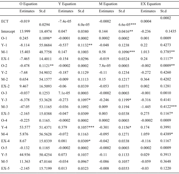
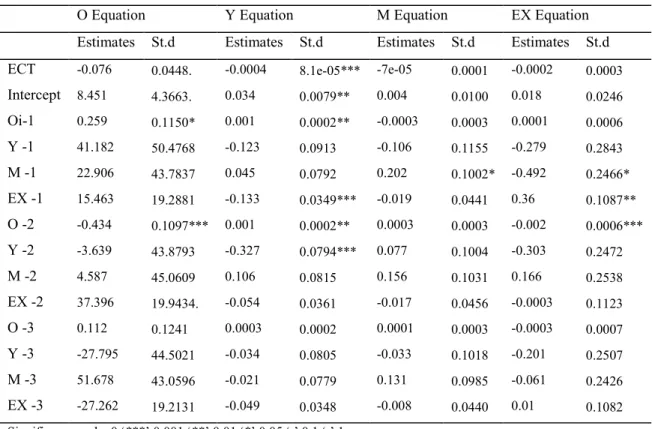
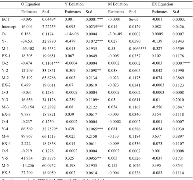
Table A.1 Parameter estimates of Reduced Form VEC Model for Australia ... 105
Table A.2 Parameter estimates of Reduced Form VEC Model for Canada ... 106
Table A.3 Parameter estimates of Reduced Form VEC Model for Chile ... 106
Table A.4 Parameter estimates of Reduced Form VEC Model for Denmark ... 107
Table A.5 Parameter estimates of Reduced Form VEC Model for Japan ... 108
Table A.6 Parameter estimates of Reduced Form VEC Model for Mexico ... 109
Table A.7 Parameter estimates of Reduced Form VEC Model for New Zealand ... 110
Table A.9 Parameter estimates of Reduced Form VEC Model for South Africa ... 112
Table A.10 Parameter estimates of Reduced Form VEC Model for South Korea ... 113
Table A.11 Parameter estimates of Reduced Form VEC Model for Switzerland ... 114
Table A.12 Parameter estimates of Reduced Form VEC Model for Sweden ... 115
Table A.13 Parameter estimates of Reduced Form VEC Model for the UK ... 116
Table A.14 OLS Estimates of the Monetary Models ... 117
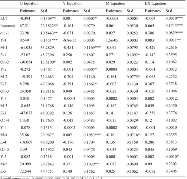
Table A.15 Parameter estimates of Reduced Form VAR Model for Canada ... 119
Table A.16 Parameter estimates of Reduced Form VAR Model for France ... 120
Table A.17 Parameter estimates of Reduced Form VAR Model for Germany ... 121
Table A.18 Parameter estimates of Reduced Form VAR Model for Italy ... 122
Table A.19 Parameter estimates of Reduced Form VAR Model for Japan ... 123
Table A.20 Parameter estimates of Reduced Form VAR Model for the UK ... 124
Table A.21 Parameter estimates of Reduced Form VAR Model for the US ... 125
Table A.22 Structural Break Tests ... 130
Table A.23 Structural Break Tests for the UK ... 130
Table A.24 Forecast Error Variance Decomposition ... 133
Table A.25 Forecast Error Variance Decompositionfor the UK. ... 133
Table A.26 Monetary Policy Responses to Structural Shocks ... 134
Table A.27 Monetary Policy Responses to Structural Shocks in the UK ... 134
Table A.28 Structural Break Tests ... 139
Table A.29 Forecast Error Variance Decomposition ... 141
Table A.30 The Role of Monetary Policy ... 142
Table A.31 The Parameter Estimates of the Reduced Form VAR with Exchange Rate ... 143
Table A.32 The Parameter Estimates of the Reduced Form VAR with Exchange Rate ... 144
Table A.33 The Parameter Estimates of the Reduced Form VAR with Exchange Rate ... 145
Table A.34 The Parameter Estimates of the Reduced Form VAR with Exchange Rate ... 146
Table A.35 The Parameter Estimates of the Reduced Form VAR with IP ... 147
Table A.36 The Parameter Estimates of the Reduced Form VAR with IP ... 148
Table A.37 The Parameter Estimates of the Reduced Form VAR with IP ... 149
Table A.38 The Parameter Estimates of the Reduced Form VAR with IP ... 150
Table A.40 The Parameter Estimates of the Reduced Form VAR with CPI ... 152 Table A.41 The Parameter Estimates of the Reduced Form VAR with CPI ... 153 Table A.42 The Parameter Estimates of the Reduced Form VAR with CPI ... 154
Acknowledgements
I would like to express my sincere appreciation to all people who have supported me during my graduate studies.
First and for most, I would like to express my profound gratitude and appreciation to my major advisor Dr. Lance Bachmeier for his guidance, encouragement, patience and availability throughout my PhD courses and research, without which none of this would be possible.
I also would like to sincerely thank my committee members: Dr. Steven Cassou, Dr. William Blankenau, Dr. Jason Bergtold, and the outside chairperson Dr. Sanjoy Das for their valuable comments.
My heartfelt and grateful appreciations are extended to my parents for their continues support, love, and encouragement throughout my life. I also want to thank my siblings, nephews, and nieces for their support and encouragement during my graduate studies. Special thanks go to my dear brother, Dr. Ibrahim Al Rasasi, and my beloved uncle, Abdarabarrasool Buessa, for their continues encouragement. Without my family’s support and encouragement, I would not be able to purse my graduate studies and accomplish this dissertation.
Last but not least, I would like to thank all my friends who have supported me during my graduate studies. In particular, I would like to extend my appreciation to: Hassan Alhashim, Mahdi Bohassan, Waheed Banafea, Abdulrahman Alqahtani, Eugenio Paulo, Soheil Nadimi, Huubinh Le, Hedieh Shadmani, Yang Jiao, Sangyun Kim, Yunyun Lv, Adeel Faheem, Atika Benaddi, Haydory Ahmad, and many others.
Dedication
Chapter 1 - Oil Prices and the US Dollar Exchange Rate: Evidence
from the Monetary Model
1.1
Introduction
Even though the monetary models of exchange rates became the standard instrument of analysis in international finance after the collapse of the Bretton Woods system in 1973, the performance of monetary models in explaining the behavior of nominal exchange rate is still unsatisfactory. Extensive surveys of traditional exchange rate models (Meese, 1990; Meese and Rose, 1991; MacDonald and Taylor, 1992; Frankel and Rose, 1995; Neely and Sarno, 2002; Chueng, et al., 2005) not only summarize the difficulties of these models, but the surveys also tend to agree that these traditional models of exchange rate are inadequate, since they fail to explain exchange rate fluctuations.
As a result, some economists, such as, Groen (2000), Cheung et al. (2005), and Chinn and Moore (2011), advocate that the flexibility of any model of exchange rate determination is necessary to incorporate other non-monetary determinants that might explain the movement of exchange rates into the monetary models of exchange rates. For instance, Cheung et al. (2005) embed other non-monetary determinants such as government debt, terms of trade and net foreign assets into monetary models of exchange rates to examine whether these non-monetary variables capture the movements of exchange rates or not. Likewise, Chinn and Moore (2011) augmented monetary model of exchange rates with order flow variables to predict exchange rates. Hunter and Ali (2014) estimated the augmented monetary model of exchange rates with the real stock price, the government consumption as a percentage of GDP, and the productivity in the traded sector to investigate exchange rate persistence.
On the other hand, several studies (Amano and Norden 1998, Chen and Rogoff 2003, Chen and Chen 2007, Narayan et al. 2008, and Uddin et al. 2014) document the influential role of energy and commodity prices on the movements of exchange rates based on atheoretical models. Hence, this motivates us to rely on some theoretical models of exchange rate determination, such as monetary models, instead of atheoretical models on which existing literature relies (see Mark 2001 for further discussion).
Because the USD is the main settlement currency in international crude oil markets, oil prices impact the USD through the US money demand function directly. Since oil-importing countries need to buy USD to purchase crude oil, their purchases increase the demand for the USD in international currency markets. Therefore, we derive an augmented flexible monetary model of exchange rates to investigate the consequences of oil prices on the movements of the USD exchange rate against 13 currencies, using quarterly data from 1986:Q1 to 2014:Q3.
In doing so, we contribute to the literature in two ways. First, examining the relationship between oil prices and the USD exchange rate in a monetary model framework is unique. Examining whether oil prices enhance the predictability of the monetary model using out-of-sample forecasts is the other contribution.
A quick preview of the results indicates a negative relationship between oil prices and the USD exchange rate against 12 currencies. Specifically, the analysis of the impulse response function shows that the depreciation rate of the USD exchange rate ranges between 0.002 and 0.018 percentage points as a result of a one-standard deviation positive shock to the real price of crude oil. Additionally, the forecast error variance decomposition analysis indicates that variation in the USD exchange rate is largely attributable to changes in the price of oil rather than monetary fundamentals.
We also compare the forecasting power of the basic model of exchange rate to the model augmented with oil prices through one-step-ahead out-of-sample forecasts evaluated by three forecasting accuracy measures. The results of the out-of-sample forecast comparisons indicate that oil prices improve the forecasting power of the monetary model of exchange rate.
This essay is organized in the following order. The next section introduces the flexible price monetary model of exchange rate, augmented with the oil price effect. Section 1.3 reviews existing literature, and section 1.4 describes the data set. Section 1.5 includes a description of the empirical methodology along with a discussion of results. Section 1.6 summarizes the results and conclusions.
1.2
The Monetary Model of Exchange Rates
The monetary model of exchange rate determination posits the link between the nominal exchange rate and a simple set of monetary fundamentals that include output, money supply, and interest rate. The basic intuition of the monetary model of exchange rates is that a country's price level is determined by its demand and supply for money and that the price level in foreign countries should be the same when it is expressed in the same currency. This makes the monetary model an attractive theoretical tool in understanding exchange rate fluctuations over time.
The monetary model of exchange rate under flexible prices consists of money market equilibrium, purchasing power parity (PPP), and uncovered interest parity (UIP). In the money market, the money demand function usually depends on the price level, p, real income, y, and the level of the interest rate, 𝑖. However, some studies augment the money demand function with other determinants, such as real effective exchange rates and the inflation rate
(Bahmani-Oskooee and Malixi, 1991), the interest rate spread (Valadkhani, 2008), opportunity cost of holding money, the real value of wealth, and investor confidence (Hall et al., 2012).
Since the US dollar is the primary invoicing currency in international crude oil markets, this in turn suggests that changes in oil prices impact the US money demand function directly. Therefore, we incorporate the real oil price (𝑂𝑡) into the US money demand function, so the
augmented money demand function of the US is given as follows:
𝑚𝑡
𝑝𝑡 = 𝐿(𝑦𝑡, 𝑖𝑡, 𝑂𝑡), (1.1) where 𝑚𝑡
𝑝𝑡 denotes the real money demand. On the other hand, we assume that the money demand function of the foreign country depends only on the price level, 𝑝, real income, 𝑦, and the level of the interest rate, 𝑖, and is given as follows:
𝑚𝑡∗
𝑝𝑡∗ = 𝐿(𝑦𝑡 ∗, 𝑖
𝑡∗). (1.2)
In money market equilibrium, money demand must equal money supply. Hence, the money demand functions given by equations (1.1) and (1.2) for both domestic and foreign countries, where asterisks denote the foreign country's variables, can be written:
𝑚𝑡− 𝑝𝑡= 𝜙𝑦𝑡− 𝜆𝑖𝑡+ 𝛿𝑂𝑡 (1.3)
𝑚𝑡∗− 𝑝
𝑡∗ = 𝜙𝑦𝑡∗− 𝜆𝑖𝑡∗, (1.4)
where 0<𝜙 <1 is the income elasticity of money demand; 𝜆 >0 is the interest rate semi-elasticity of money demand; and 𝛿 > 0 is the oil price elasticity. This relationship is true because crude oil is priced in US dollars and higher oil prices increase demand for the US dollar, resulting in an appreciation of the US dollar. All variables, with the exception of interest rates, are expressed in logarithm form. Under the flexible price monetary model, the standard PPP relationship is assumed to hold continuously:
𝑒𝑡 = 𝑝𝑡− 𝑝𝑡∗, (1.5)
where 𝑒𝑡 represents the nominal exchange rate measured in foreign currency to domestic currency. Since the price levels determine the domestic and foreign money supplies, as in equation (1.5), the price level functions can be presented as follows:
𝑝𝑡= 𝑚𝑡− 𝜙𝑦𝑡+ 𝜆𝑖𝑡− 𝛿𝑂𝑡 (1.6)
𝑝𝑡∗ = 𝑚𝑡∗− 𝜙𝑦𝑡∗+ 𝜆𝑖𝑡∗. (1.7)
Therefore, we substitute equations (1.6) and (1.7) into equation (1.5) to obtain the exchange rate,
𝑒𝑡, as follows:
𝑒𝑡 = (𝑚𝑡− 𝜙𝑦𝑡+ 𝜆𝑖𝑡− 𝛿𝑂𝑡) − (𝑚𝑡∗− 𝜙𝑦
𝑡∗− 𝜆𝑖𝑡∗) . (1.8)
This can be simplified to:
𝑒𝑡 = (𝑚𝑡− 𝑚𝑡∗) − 𝜙(𝑦𝑡− 𝑦𝑡∗) − 𝛿𝑂𝑡+ 𝜆(𝑖𝑡− 𝑖𝑡∗). (1.9)
Note that the monetary model of the exchange rate under flexible prices assumes that UIP, which equates the interest rate differential between two countries to the future change in exchange rate, holds. The UIP condition is given by the following equation:
𝑖𝑡− 𝑖𝑡∗= 𝐸(∆𝑒𝑡+1|Ω𝑡), (1.10)
where 𝐸(. |Ω𝑡) represents the expectation of future change in nominal exchange rate based on the information set Ω at the current time period. Then, equation (1.9) becomes
𝑒𝑡 = (𝑚𝑡− 𝑚𝑡∗) − 𝜙(𝑦𝑡− 𝑦𝑡∗) − 𝛿𝑂𝑡+ 𝐸(∆𝑒𝑡+1|Ω𝑡) . (1.11)
If 𝑒𝑡 is 𝐼 (0) or 𝐼 (1), then ∆𝑒𝑡+1 will equal to zero in the steady state, as in Rapach and Wohar (2002). Thus, equation (1.11) will become:
𝑒𝑡 = (𝑚𝑡− 𝑚𝑡∗) − 𝜙(𝑦𝑡− 𝑦𝑡∗) − 𝛿𝑂𝑡 . (1.12)
Based on equation (1.12), we can infer that a rise in the domestic money supply relative to the foreign money supply, ceteris paribus, leads to the appreciation of the nominal exchange
rate (𝑒𝑡). On the other hand, a rise in domestic output relative to foreign output, ceteris paribus,
causes the depreciation of the nominal exchange rate (𝑒𝑡). Regarding the impact of oil price increases, a rise in oil prices leads to the depreciation of the nominal exchange rate (𝑒𝑡).
1.3
Literature Review
In the seminal work of Meese and Rogoff (1983), they document the failure of various monetary models and time series models of exchange rate determinations in predicting the movements of exchange rates. Since then, there has been extensive research attempting to explain the movements of exchange rates. This, in turn, encourages researchers to look for other factors that might be able to explain and to predict exchange rate movements. Lastrapes (1992) identifies three real shocks, productivity growth, government budget deficit, and real oil prices, to explore their effects on real exchange rates. He documents evidence showing that these shocks explain more than 80% of exchange rate variations in the long run.
Clarida and Gali (1994) employ the Blanchard-Quah identification scheme to explore the consequences of real shocks, including demand, supply, and money, on the bilateral real exchange rate of the US dollar against the currencies of Canada, Germany, Japan, and the UK. They conclude that real shocks contribute to the variation in real exchange rate by more than 50% of the variance of the real exchange rate variability. Other authors (Throop, 1993; Evans and Lothian, 1993; and Zhou, 1995) confirm that non-monetary shocks play an influential and significant role in explaining the variations of exchange rates.
Moreover, other studies, based on atheoretical models, document the explanatory power of oil prices in capturing the movements of exchange rates. Amano and Norden (1998) examine the essential role of oil prices on real exchange rates of three major currencies with monthly data over the period 1973:01 to 1993:06. They find evidence supporting the existence of a stable long
run relationship between oil prices and real exchange rates. Their analysis indicates that higher oil prices lead to the appreciation of the US dollar and the depreciation of the German Mark and the Japanese Yen.
Chaudhuri and Daniel (1998) use the data of 16 OECD countries to examine the effects of oil prices on the US real exchange rate. They report that oil prices can explain the fluctuations of US real exchange rate, since both oil prices and real exchange rates have the same nonstationary behavior. They also find evidence supporting the idea that higher oil prices lead to the appreciation of the US dollar against all countries. Sadorsky (2000) uses various energy prices, including crude oil prices, to examine their impacts on the trade-weighted US exchange rate. He reports evidence supporting the existence of a long run relationship between energy prices and the US dollar exchange rate. Sadorsky also documents the negative relationship between energy prices and the USD exchange rate.
Akram (2004) studies the possibility of a non-linear cointegration relationship between oil prices and the Norwegian exchange rate. He finds evidence supporting the notion of a negative relationship between oil prices and exchange rate; he also points out that this relationship varies with the level and with the trend in oil prices. Chen and Chen (2007) use panel cointegration techniques to investigate the relationship between real oil prices and the US dollar exchange rates against G7 countries. Their evidence indicates not only the presence of a cointegration relationship between oil prices and exchange rates, but also confirms that oil prices are able to predict the movements of exchange rates.
Narayan, et al. (2008) employ both the GARCH and exponential GARCH models to investigate the impact of oil prices on the nominal exchange rate of the Fiji Islands. They find evidence confirming the negative relationship between oil prices and the US dollar relative to the
Fiji exchange rate. Jahan-Parvar and Mohammadi (2008) examine the relationship between oil prices and the real exchange rate for 14 oil-producing countries based on an autoregressive distributed lag model. Their evidence indicates the existence of a stable long run relationship between oil prices and exchange rate, confirming the validity of the Dutch disease hypothesis. In an alternative paper, Mohammadi and Jahan-Parvar (2012) employ threshold and momentum-threshold models to explore the validity of the Dutch disease hypothesis for 13 oil-exporting countries. They find evidence supporting the validity of the Dutch disease only for three countries; in other words, the US dollar tends to depreciate relative to the Bolivian boliviano, Mexican peso, and Norwegian krone. Other studies (Huang and Guo, 2007; Thalassinos and Politis, 2012; and Uddin et al., 2014) also document the essential role of oil prices in explaining the behavior of exchange rates.
1.4
Data
We use quarterly data over the period 1986:Q1 to 2014:Q3 for the nominal exchange rate of the US dollar, West Texas intermediate crude oil prices, GDP, and money supply for the following 14 countries: Australia, Canada, Chile, Denmark, Japan, Mexico, New Zealand, Norway, South Africa, South Korea, Sweden, Switzerland, the United Kingdom (U.K.), and the United States of America (US). The composition of the sample is determined by data availability. In addition, these countries are major trade partners of the US, and the currencies of these countries are actively traded in the international currency market.
The data for GDP and oil prices are obtained from the International Financial Statistics (IFS) database of the International Monetary Fund (IMF) and Federal Reserve Bank of St. Louis, respectively. The nominal exchange rate is measured as US Dollar per one unit of foreign currency; thus, an increase in the nominal exchange rate means a depreciation of the USD.
Money supply is measured by the broad money supply, M3. The nominal exchange rate and money supply data are obtained from the Organization for Economic Co-operation and Development (OECD) database. It is also essential to emphasize that all the data are expressed in logarithm form.
1.5
Empirical Methodology and Results
1.5.1Preliminary Investigation
The first step of the analysis is to ascertain the order of integration of the economic variables. To do so, we rely on some standard unit root tests, the Augmented Dickey–Fuller “ADF” (1979), the Phillips Perron “PP” (1988), and the Kwiatkowski, Phillips, Schmidt and Shin “KPSS” (1992) tests, to ensure the stationarity of the economic variables1. The results of these tests, as presented in Tables 1.1 – 1.6, confirm the nonstationarity of all variables in their levels and the stationarity of the variables in their first difference.
Since our economic variables are integrated of order one, or I (1), then some of these variables may be cointegrated. To check this, we apply the popular cointegration tests developed by Johansen and Juselius (1990). These tests also enable us to gauge the adequacy of modeling the US nominal exchange rate as a function of oil prices and monetary fundamentals. Table 1.7 presents the results of the Johansen and Juselius (1990) cointegration tests2, which consist of the Trace and the Maximum Eigenvalue tests. Both the Trace and the Maximum Eigenvalue tests confirm the existence of at least one cointegration relationship among our economic variables.
Before proceeding in our analysis, we also assess the stability of the existing cointegration relationship between the USD exchange rate, oil prices, and monetary
1 The unit root tests were done in R (version 3.1.2) using functions ur.df, ur.pp, and ur.kpss from package urca
(version 1.2-8).
fundamentals. To do so, we employ the Quandt–Andrews unknown breakpoint tests developed by Andrews (1993) and Andrews and Ploberger (1994). The essential idea behind the Quandt– Andrews unknown breakpoint does not assign any information regarding the breakpoints prior to the estimation and identifies the breakpoints by comparing the residuals before and after the presumed point of break for every time period. The test statistics are summarized as Sup F, Ave F, and Exp F that all share the same null hypothesis of no structural change. To obtain these test statistics3, we estimate the following vector error correction model via OLS.
𝑒𝑗,𝑡= 𝛼 + ∑𝑘𝑖=1𝛽𝑖𝑒𝑗,𝑡+ 𝛾(𝑚𝑡− 𝑚𝑡∗) + 𝛿(𝑦𝑡− 𝑦𝑡∗) + ∑𝑘𝑖=1𝜃𝑖∆𝑂𝑖𝑙𝑡−𝑖+ 𝜙𝐸𝐶𝑇𝑡−1+ 𝜀𝑡 , (1.13)
where 𝑒𝑗,𝑡 is the USD exchange rate against the foreign country j at time t; (𝑚𝑡− 𝑚𝑡∗) denotes
the US money supply relative to foreign money supply; (𝑦𝑡− 𝑦𝑡∗) denotes the US output relative to the foreign output; ∆𝑂𝑖𝑙𝑡 is the percentage change of oil price at time t. 𝐸𝐶𝑇𝑡−1 is the error correction term at time period 𝑡 − 1 , the lag length k is chosen based on the Akaike information criteria “AIC”, and 𝜀𝑡 is the error term. Note that the error correction term is given as follows:
𝐸𝐶𝑇𝑡 = 𝑒𝑗,𝑡− 𝛼0− 𝛼1(𝑚𝑡− 𝑚∗𝑡) − 𝛼2(𝑦𝑡− 𝑦𝑡∗) − 𝛼3𝑂𝑖𝑙𝑡. (1.14)
In Table 1.8, we present the estimated break date and the corresponding structural break tests with asymptotic p-values computed by Hansen's (1997) approximation. We fail to reject the null hypothesis of no structural break, confirming the stability of the parameter estimates of the exchange rate’s vector error correction equation at 1%, 5%, or 10% significance levels.
3 The structural break tests were done in R (version 3.1.2) using function sctest from package strucchange (version
Table 1.1 Augmented Dickey Fuller (1979) Unit Root Test. Level Data First Difference Data
None Trend Drift None Trend Drift Oil 0.8698 -3.012 -1.1935 -9.078 -9.1979 -9.2325 Gross Domestic Product:
Australia 6.5419 -2.3031 -0.5065 -3.5225 -6.4543 -6.4688 Canada 4.0823 -2.4174 -0.7211 -4.1401 -6.1275 -6.1246 Chile 4.6102 -2.4168 -1.942 -8.4519 -11.108 -10.8579 Denmark 2.3055 -1.1268 -1.3505 -8.7677 -9.1232 -9.1092 Japan 3.7074 -1.7792 -4.0849 -5.5998 -7.5056 -6.5805 Mexico 4.2012 -2.6929 -0.5433 -6.8654 -7.9851 -7.9972 New Zealand 4.3364 -2.7699 -0.6646 -10.1054 -13.214 -13.1972 Norway 2.3035 -2.9596 -1.1966 -14.5024 -15.8873 -15.8152 South Africa 3.5054 -1.7922 0.8408 -4.1502 -5.4712 -5.2679 South Korea 4.1979 -1.8482 -2.1259 -10.0935 -12.3452 -12.0334 Sweden 1.6451 -3.5466 -2.1684 -7.0928 -7.3317 -7.3007 Switzerland 3.934 -2.8098 -0.0588 -4.4029 -5.7762 -5.7868 U.K. 3.0812 -1.812 -1.3912 -2.7071 -3.8572 -3.7585 US 5.5083 -1.0612 -1.8954 -3.4698 -6.0906 -5.8485
Table 1.2 Augmented Dickey Fuller (1979) Unit Root Test. Money Supply (M3)
Level Data First Difference Data None Trend Drift None Trend Drift Australia 3.6408 -2.0918 -0.3351 -1.8229 -4.4249 -4.435 Canada 4.718 -1.6765 -0.2038 -1.7757 -4.9107 -4.9332 Chile 1.2241 -3.6582 -4.5176 -1.5039 -3.7176 -2.4373 Denmark 2.3347 -3.113 -0.1339 -6.028 -6.8047 -6.8172 Japan 1.306 -4.3613 -2.9862 -2.0737 -2.6478 -2.494 Mexico 0.4106 -6.1197 -3.2997 -2.5028 -3.1465 -2.9138 New Zealand 5.7351 -1.7899 -1.4793 -2.8367 -5.3779 -5.2829 Norway 4.47 -2.5301 -0.8581 -2.6573 -5.6567 -5.6297 South Africa 3.328 -1.0243 -2.1015 -1.9549 -4.8938 -4.5382 South Korea 1.5133 -4.0562 -6.7109 -1.7086 -4.1111 -2.2977 Sweden 4.614 -2.077 -0.5132 -4.0539 -6.0018 -6.0342 Switzerland 3.9112 -2.0066 -0.1965 -2.7967 -4.4453 -4.4526 U.K. 4.1134 -0.6535 -1.9547 -2.8572 -4.6978 -4.3702 US 5.3074 -1.11 1.7401 -2.3288 -5.8045 -5.2695
Table 1.3 Augmented Dickey Fuller (1979) Unit Root Test. Nominal Exchange Rate
Level Data First Difference Data None Trend Drift None Trend Drift Australia -1.2583 -2.2589 -1.8821 -7.6756 -7.6364 -7.687 Canada -1.2398 -1.7261 -1.4553 -7.1251 -7.1048 -7.1366 Chile 1.6357 -2.144 -2.6737 -7.0038 -7.6849 -7.3618 Denmark -0.7906 -2.816 -2.6585 -7.3969 -7.3768 -7.3972 Japan -0.8481 -2.7983 -2.5265 -8.7141 -8.797 -8.7462 Mexico 0.7803 -3.8813 -4.2748 -5.2182 -6.1635 -5.6317 New Zealand -1.0837 -2.4475 -1.8431 -6.6408 -6.6353 -6.6788 Norway -0.4238 -2.6093 -2.4949 -7.8643 -7.8018 -7.8378 South Africa 1.4554 -2.0092 -0.9556 -6.8934 -7.1724 -7.2092 South Korea 0.1244 -2.6026 -1.9109 -7.4904 -7.4288 -7.4622 Sweden -0.1824 -2.5621 -2.5363 -7.5338 -7.4661 -7.4972 Switzerland -1.8783 -2.4719 -1.6087 -7.7944 -7.855 -7.889 U.K. -0.5444 -3.3902 -3.4068 -8.0782 -8.0039 -8.0409
Table 1.4 Phillips and Perron (1981) and Kwiatkowski et al (1992) Unit Root Test. Phillip and Perron (1981) Test Kwiatkowski-Phillips-Schmidt-Shin (1992) Test
Level First Difference Level First Difference Constant Trend Constant Trend Constant Trend Constant Trend Oil -0.698 -2.737 -8.887 -8.833 2.082 2.082 0.073 0.038 Gross Domestic Product:
Australia -0.388 -2.289 -9.162 -9.137 2.882 0.182 0.075 0.069 Canada -0.548 -1.936 -6.465 -6.457 2.860 0.193 0.078 0.065 Chile -1.870 -2.727 -19.466 -20.795 2.315 0.492 0.276 0.030 Denmark -1.533 -4.755 -34.783 -35.685 2.270 2.270 0.119 0.041 Japan -3.930 -1.473 -9.827 -10.729 2.461 0.641 1.007 0.077 Mexico -0.774 -6.522 -23.841 -23.768 2.361 2.361 0.032 0.021 New Zealand -1.157 -3.269 -14.988 -14.954 2.698 0.207 0.108 0.049 Norway -1.006 -3.849 -22.158 -22.499 2.838 0.461 0.123 0.067 South Africa 0.947 -1.299 -6.333 -6.456 2.735 0.643 0.307 0.083 South Korea -2.512 -3.113 -30.438 -34.651 2.794 0.689 0.445 0.017 Sweden -2.956 -9.393 -41.330 -43.970 1.625 0.306 0.312 0.146 Switzerland 0.031 -2.442 -7.147 -7.129 2.816 0.174 0.054 0.042 U.K. -1.806 -1.470 -5.033 -5.170 2.376 2.37 0.281 0.082 US -1.267 -0.818 -8.501 -8.678 2.847 0.491 0.255 0.096
Table 1.5 Phillips and Perron (1981) and Kwiatkowski et al (1992) Unit Root Test. Phillip and Perron (1981) Test Kwiatkowski-Phillips-Schmidt-Shin (1992) Test
Level First Difference Level First Difference Constant Trend Constant Trend Constant Trend Constant Trend Money Supply (M3): Australia -0.462 -1.672 -4.736 -4.716 2.373 2.373 0.109 0.116 Canada -0.236 -1.460 -5.628 -5.603 2.369 2.369 0.192 0.195 Chile -8.180 -3.904 -2.753 -4.569 2.216 2.216 1.606 0.380 Denmark -0.064 -2.345 -6.590 -6.575 2.339 2.339 0.103 0.078 Japan -6.239 -4.952 -2.193 -2.515 2.116 2.116 1.075 0.286 Mexico -7.962 -8.152 -2.331 -2.994 2.269 2.269 1.296 0.283 New Zealand -1.844 -2.381 -8.651 -8.787 2.403 2.403 0.261 0.059 Norway -0.704 -1.961 -5.875 -5.883 2.392 2.392 0.085 0.076 South Africa -1.709 -0.788 -6.247 -6.599 2.392 2.392 0.301 0.114 South Korea -14.220 -4.495 -2.835 -6.528 2.274 2.274 2.032 0.391 Sweden -0.628 -2.028 -7.639 -7.612 2.350 2.350 0.077 0.077 Switzerland 0.077 -1.356 -5.334 -5.303 2.326 2.326 0.220 0.209 U.K. -2.759 -1.830 -7.164 -7.533 2.304 2.304 0.512 0.143 US 1.798 -0.699 -5.748 -6.047 2.382 2.382 0.479 0.112
Table 1.6 Phillips and Perron (1981) and Kwiatkowski et al (1992) Unit Root Test. Phillip and Perron (1981) Test Kwiatkowski-Phillips-Schmidt-Shin (1992) Test
Level First Difference Level First Difference Constant Trend Constant Trend Constant Trend Constant Trend Nominal Exchange Rate:
Australia -1.543 -1.906 -7.861 -7.838 0.737 0.737 0.087 0.055 Canada -1.271 -1.494 -7.531 -7.495 0.896 0.896 0.114 0.108 Chile -2.970 -2.035 -7.901 -8.093 1.647 1.647 0.492 0.080 Denmark -2.624 -2.697 -8.268 -8.252 0.829 0.829 0.090 0.072 Japan -2.953 -3.117 -9.025 -9.058 1.394 1.394 0.163 0.067 Mexico -5.154 -4.224 -6.999 -7.697 2.035 2.035 0.747 0.117 New Zealand -1.565 -2.053 -7.247 -7.235 0.862 0.862 0.072 0.050 Norway -2.116 -2.240 -8.428 -8.384 0.600 0.600 0.056 0.058 South Africa -1.010 -1.939 -8.561 -8.523 2.108 2.108 0.075 0.059 South Korea -1.665 -2.239 -7.680 -7.643 1.370 1.370 0.074 0.071 Sweden -2.150 -2.181 -7.598 -7.559 0.455 0.455 0.061 0.060 Switzerland -1.714 -2.472 -8.772 -8.730 1.546 1.546 0.071 0.075 U.K. -2.972 -2.963 -8.239 -8.190 0.132 0.132 0.042 0.041
Table 1.7 Johansen and Juselius (1990) Cointegration Test.
Trace Test Eigenvalue Max Test
𝑟 ≤ 0 𝑟 ≤ 1 𝑟 ≤ 2 𝑟 ≤ 3 𝑟 ≤ 0 𝑟 ≤ 1 𝑟 ≤ 2 𝑟 ≤ 3 Australia 49.70*** 27.16 15.22 4.53 25.59*** 11.94 10.70 4.53 Canada 51.19*** 25.43 12.20 0.90 25.76*** 13.23 11.30 0.90 Chile 85.98** 43.28** 7.12 3.32 42.70** 36.16** 3.80 3.32 Denmark 49.36** 28.49 13.75 6.37 20.87 14.74 7.37 6.37 Japan 87.58** 33.75*** 15.78 4.95 53.83** 17.97 10.83 4.95 Mexico 62.81** 30.89 13.20 4.89 31.92** 17.69 8.30 4.89 New Zealand 78.74** 31.46 15.67 4.93 47.28** 15.79 10.73 4.93 Norway 61.35** 24.22 14.42 5.75 37.12** 9.80 8.67 5.75 South Africa 87.34** 36.61** 10.83 2.77 50.74** 25.77** 8.06 2.77 South Korea 106.21** 46.99** 17.02 3.84 59.21** 29.97** 13.18 3.84 Sweden 61.61** 21.09 8.65 2.01 40.52** 12.44 6.64 2.01 Switzerland 90.97** 41.97** 21.47** 7.36 49.00** 20.49*** 14.11*** 7.36 U.K. 57.49** 24.85 9.76 2.63 32.64** 15.09 7.12 2.63 * (**) (***) Indicate the rejection of the null at 1%, 5%, and 10% level of significance respectively.
Table 1.8 Structural Break Tests.
Break Date Ave F Sup F Exp F Australia 2008:Q4 5.14 (0.59) 14.3 (0.29) 3.68 (0.47) Canada 2007:Q2 6.51 (0.35) 10.56 (0.65) 3.66 (0.48) Chile 2002:Q4 8.29 (0.15) 21.12 (0.03) 7.17 (0.04) Denmark 1990:Q1 5.98 (043) 11.92 (0.49) 3.59 (0.50) Japan 1994:Q3 3.48 (0.90) 14.12 (0.30) 3.19 (0.61) Mexico 1993:Q2 3.92 (0.83) 14.09 (0.30) 3.74 (0.46) New Zealand 2007:Q2 12.31 (0.03) 18.59 (0.08) 7.29 (0.04) Norway 1991:Q3 7.28 (0.24) 14.88 (0.24) 5.16 (0.19) South Africa 2001:Q2 4.84 (0.65) 13.82 (0.32) 3.49 (0.65) South Korea 1996:Q3 2.72 (0.98) 20.09 (0.06) 5.72 (0.13) Sweden 2007:Q4 9.39 (0.08) 17.45 (0.12) 5.80 (0.12) Switzerland 1993:Q4 6.24 (0.38) 14.51 (0.27) 5.05 (0.20) U.K. 2008:Q4 9.42 (0.08) 14.96 (0.34) 5.53 (0.14) Numbers in parenthesis are p-values.
1.5.2The Vector Error Correction Model
It is common in the literature to rely on Vector Autoregressive (VAR) models as empirical tools to investigate the effects of oil price shocks on various macroeconomic and financial variables. However, the standard VAR model is a reduced form model. Interpreting the results obtained from the reduced form is often impossible, unless the reduced form VAR is linked to an economic model. In other words, when economic theory provides an explanation linking forecast errors and fundamental shocks, then we call the resulting model a Structural Vector Autoregressive (SVAR) model. In case there exists a cointegration relationship among
the economic variables, then it is possible to apply the SVAR technique to vector error correction models (VECM) with cointegrated variables.
The analysis of a structural vector error correction (SVEC) model starts from the reduced form standard 𝑉𝐴𝑅 (𝑝) model:
𝑋𝑡 = 𝐴1𝑋𝑡−1+ 𝐴2𝑋𝑡−2+ ⋯ + 𝐴𝑝𝑋𝑡−𝑝+ 𝑢𝑡 , (1.15)
where 𝑋𝑡 = (𝑂𝑡, 𝑌𝑡, 𝑒𝑡, 𝑀𝑡)′ is a 𝑘 × 1 vector of observable variables consisting of real oil price,
domestic output relative foreign output, nominal exchange rate of the USD, and domestic money supply relative foreign money supply. 𝐴′𝑖𝑠 are (𝑘 × 𝑘) coefficient matrices, and 𝑢𝑡 is a (𝑘 × 1)
vector of unobservable error terms with 𝑢𝑡~(0, ∑ )𝑢 . The lag order, 𝑝, is determined based on the
Akaike Information Criterion (AIC).
By assuming that the variables are at most difference stationary, then the reduced form VAR model can be written as a VECM of the form:
𝐵0∆𝑋𝑡= Π∗𝑋
𝑡−1+ Γ1∗Δ𝑋𝑡−1+ ⋯ + Γ𝑝−1∗ Δ𝑋𝑡−𝑝+1+ 𝜀𝑡, (1.16)
where ∆ denotes the first difference of 𝑋𝑡−𝑘, Γ∗′𝑠 are (𝑘 × 𝑘) matrices of short run coefficients. Π∗ is the structural matrix, and 𝜀𝑡 is (𝑘 × 1) structural form error with zero mean and covariance matrix 𝐼𝐾. 𝐵0 is a (𝑘 × 𝑘) matrix of contemporaneous relations among the variables in 𝑋𝑡. If we assume that the 𝐵0 matrix is invertible, then we can rewrite equation (1.16) as follows:
∆𝑋𝑡= Π𝑋𝑡−1+ Γ1Δ𝑋𝑡−1+ ⋯ + Γ𝑝−1Δ𝑋𝑡−𝑝+1+ 𝑢𝑡, (1.17)
where Π𝑡 = 𝐵0−1Π∗ and Γ
𝑗 = 𝐵0−1Γ𝑗∗ for 𝑗 = 1, … , 𝑝 − 1 . The 𝑢𝑡= 𝐵0−1𝜀𝑡 relates the reduced
form disturbance, 𝑢𝑡′, to the underlying structural errors 𝜀𝑡. When Π has a reduced rank of 𝑟 ≤ 𝑘 − 1, then Π = 𝛼𝛽′ where 𝛼 and 𝛽 are (𝑘 × 𝑟) matrices consisting of the long run relationship
error with zero mean and covariance matrix Σ𝑢. When we substitute Π into equation (1.17), we
obtain the model in error correction form as follows:
∆𝑋𝑡= 𝛼𝛽′𝑋𝑡−1+ Γ1Δ𝑋𝑡−1+ ⋯ + Γ𝑝−1Δ𝑋𝑡−𝑝+1+ 𝑢𝑡. (1.18)
Because the reduced form residuals, 𝑢𝑡′𝑠, are strongly correlated, it is difficult to eliminate the effects of a single shock on the whole system unless some restrictions are imposed on the system. To do so, we multiply both sides by 𝐵0 in order to obtain,
𝐵0𝑢𝑡= 𝜀𝑡 (1.19)
Σ = 𝐵0−1Σ𝜀(𝐵0)′, (1.20)
where Σ, 𝐵0, and Σ𝜀 are all (k × k) matrices. Since the literature has proposed a number of different exact identification schemes, we rely on the most popular Cholesky4 identification scheme to obtain an exact identification of Σ𝜀 requiring the imposition of 𝑘 × (𝑘 − 1)/2
additional restrictions on 𝐵0−1. Under the Cholesky scheme, the ordering of the variables is
crucial for the structural economic interpretation of the VECM. Therefore, we order the variables as follows: real oil price, relative output, nominal exchange rate of the USD, and relative money supply; 𝑋𝑡= (𝑂𝑡, 𝑌𝑡, 𝑒𝑡, 𝑀𝑡)′.
The economic justification of this recursive ordering is based on four reasons. Since the US is a price taker in the oil market, and the price of crude oil is determined by global demand and supply conditions, then the relative output, exchange rate, and relative money supply will have negligible effects on it. Hence, the price of crude oil is assumed to be exogenous. However, the price of oil can have a contemporaneous effect on the other variables. In other words, a rise
4Sims (1980) introduced Cholesky decomposition. It is a recursive identification scheme assuming that the covariance matrix is diagonal, and 𝐵 matrix is a lower triangular matrix by imposing 𝑘 × (𝑘 − 1)/2 extra restrictions to ensure the identification of
(decline) of oil price would increase (decrease) the cost of production, since crude oil is used as an input in the production process and the distribution process of goods and services.
Second, relative output is assumed to not respond contemporaneously to any changes in relative money supply and exchange rate. Kim and Ying (2007) documents that the information about money supply and exchange rate is only available with a lag, since they are not observable within a month. Third, we impose that nominal exchange rates do not respond to changes in relative money supply. Fourth, since the relative money supply is a policy variable and controlled by monetary authorities, we allow the relative money supply to respond to changes in the other variables.
Once we estimate the VECM5, we compute impulse response functions6 to examine the effects of each structural shock on the other variables. Therefore, to examine the dynamic effects of each structural shock on the movements of the USD nominal exchange rates, we compute the impulse responses with a one standard deviation band.
The analysis of impulse responses is essentially used to trace out the dynamic responses of the equations in the VECM to a set of identified structural shocks. In essence, impulse response analysis enables us to trace out the dynamic impact of changes in each of the variables in the VECM over time. In addition, the identification assumptions impose that the shock is a one-standard deviation movement of one of the shocks.
5 The estimates of VECM were done in R (version 3.1.2) using function VECM from package vars (version 1.5-2);
the parameter estimates of VECM are attached in the appendix.
6 The estimated impulse responses were done in R (version 3.1.2) using function irf from package vars (version
1.5.3Impulse Response Function Results
Figures 1.1 – 1.4 display the response of the USD exchange rate to the identified structural shocks with a one standard deviation band.
The derived monetary model of exchange rates suggests a negative link between oil prices and the USD exchange rates. Figure 1.1 illustrates the response of the USD exchange rate to real oil price shock and indicates that higher oil prices are associated with the depreciation of the USD exchange rate against all currencies, except the Australian currency. In other words, the plotted impulses indicate that a one-standard deviation shock to the real price of oil is followed by a depreciation of the USD exchange rate against twelve currencies, and the depreciation rate ranges between 0.002 and 0.018 percent points. On the other hand, the USD against the Australian dollar experiences an appreciation rate of 0.016 percent point as a result of a one-standard deviation shock to the real price of oil.
It is also worthy to note that the results indicating the negative relationship between oil prices and the USD exchange rates are consistent with the findings of previous studies, such as Chaudhuri and Daniel (1998), Sadorsky (2000), Chen and Chen (2007), and Uddin et al. (2014).
The monetary model of exchange rates indicates a negative relationship between the nominal exchange rate and relative output. The plotted impulses with a one-standard deviation band, as shown in Figure 1.2, illustrate the response of the USD exchange rate to real output shocks. In particular, a positive shock to relative output causes the USD exchange rate to increase (depreciate) immediately against four currencies whereas it declines (appreciates) immediately against nine currencies. For example, we find the immediate response of a one-standard deviation shock to relative output causes the nominal exchange rate to appreciate by 0.002 and 0.008 percent points for Chile and Sweden respectively.
Likewise, the derived monetary model of exchange rates suggests a positive relationship between relative money supply and nominal exchange rates. Figure 1.3 illustrates the responses of the USD exchange rate to a positive shock to the relative money supply. We find the responses of the USD to a positive shock to the nominal money supply indicate the appreciation of the USD against ten currencies whereas the USD depreciates against four currencies. For instance, we find that the immediate response of a one-standard deviation shock to the relative money supply leads to the depreciation of the USD against the Mexican peso by 0.016 percent points.
It is worthy to document that the reported findings regarding the impacts of monetary fundamentals on the movements of the USD exchange rate are consistent with the findings of Rapach and Wohar (2004) for Australia, Canada, Denmark, and Sweden, Lizardo and Mollick (2010) for Mexico and the UK, Hunter and Ali (2015) for Japan, and Bruyn et al. (2013) for south Africa.
Lastly, the impact of a positive shock to the exchange rate to itself is shown in Figures 1.4 The plotted impulses with a one-standard deviation bands show that the USD rises (depreciates) during the first two quarters then starts declining (appreciating) in the remaining time period against most currencies. The plotted impulses indicate that the USD increases (depreciates) against the currencies of Canada, Mexico, Norway, and South Africa until the fourth or fifth quarter, and then it starts to decrease (appreciate) or stabilize until the end of the time period. We find the response of the USD against the New Zealand currency to be positive (depreciating) until the fifth quarter, and then it stabilizes over the remaining period. To summarize, we find that a one-standard deviation shock to the USD exchange rate leads to the depreciation of the USD exchange rate within a range of 0.020 and 0.041 percent points.
These results have implications for policy makers, economic researchers, and traders. The USD depreciation, as suggested by economic analysis, has positive and negative effects on the US economy. First, the depreciation of the USD helps in reducing the US trade deficit, since the fall of the USD increases the price competitiveness of US exports in foreign markets and decreases the price competitiveness of foreign goods in the US market. This, in turn, will increase employment since there will be less demand subtracted from the economy. In other words, higher US exports will improve domestic economic activity and improve employment, while lower imports of foreign goods means less domestic spending on foreign goods resulting in a boost to the domestic economy and employment.
Second, world commodity prices tend to increase as a result of the depreciation of the US dollar. For instance, when the USD experienced a sharp depreciation between 2002 and 2007, there was a sharp surge in gold prices from $300 per ounce to more than $600 per ounce, and crude oil price increased from $20 per barrel to approximately $140 per barrel. The index of non-fuel commodity prices also experienced an increase by 85%. Third, the depreciation of the USD discourages foreign investors to hold dollar assets due to its low expected return. Finally, the depreciation of the USD reduces the US net foreign debt. This is possible because US foreign assets and US foreign liabilities are denominated in foreign currencies and USD, respectively. So, a real depreciation of the USD tends to raise the value of US external assets, while the value of US external liabilities does not rise. Consequently, this reduces the US external debt.
Figure 1.1 The Response of the USD Exchange Rate to Oil Price Shocks
Figure 1.3 The Response of the USD Exchange Rate to Relative Money Supply Shocks
Figure 1.4 The Response of the USD Exchange Rate to Exchange Rate Shocks
1.5.4Forecast Error Variance Decomposition Analysis
While the impulse response function illustrates the qualitative response of the USD exchange rate to shocks in the price of oil and other structural shocks, the forecast error variance decomposition7 (FEVD) illustrates the relative importance of the structural shocks in explaining the variations of the USD exchange rate and the variations of other variables.
Table 1.9 presents the contribution of all structural shocks on the USD exchange rate based on the forecast error variance decomposition. Because the price of oil is ordered first in the VEC model, this decomposition assumes that the initial period has all variance in the forecasts attributed to the price of oil and none to the other variables. Therefore, we find that as the forecast horizon increases, there is more variation attributed to the other changes based on the correlation of the changes and the dynamics of the system.
The forecast variation helps us to understand the important role of oil price shocks and other structural shocks in determining the movements of the USD exchange rate. It is evident from the results shown in Table 1.9 that the variation of the USD exchange rate is attributed largely to its own shocks, and as the forecast horizon increases, the contribution of the exchange rate shock on the movements of the USD declines.
Among the other structural shocks, we find the variation in the USD exchange rate is driven to some extent by oil price changes. In particular, we find that between 0.27% and 22.91% is attributed to the change in oil price during the first quarter. After eight quarters, or two years, the results indicate that the variation in the USD exchange rate attributed to the change in oil prices lies within a range of 0.34% and 15.02%. This indicates a decline of the contribution of oil prices in explaining the movements of the USD exchange rates. However, we find that, as the
forecast horizon increases, changes in oil prices yield more variation in the value of the USD against seven currencies. The USD variation lies approximately within a range of 6.01% and 15.12%.
Furthermore, the FEVD results indicate that the impact of monetary fundamentals on the USD variation tends to increase as the forecast horizon increases for most countries. However, the change attributable to monetary fundamentals is relatively small compared to the change attributable to the movement in oil prices. For example, the pattern of the forecast variation indicates that shocks to relative output (money supply) explain the USD fluctuations after twelve quarters or three years, within the range of 0.39% and 53.61% (0.24% and 16.79%).
In the case of the USD against the Japanese yen, changes in relative output play a larger role than changes in the relative money supply and oil prices. Strictly speaking, we find that changes in the value of the USD against the Japanese yen are attributed to changes in the relative output by approximately 0.78%. However, about 0.54% of the USD variation is attributable to shocks to the price of oil after one year. As the forecast horizon increases, the contribution of the oil price and relative output shocks decreases; in other words, we find that oil and relative output shocks contribute to explaining roughly 0.34% and 0.39%, respectively, of the movements of the USD exchange rate.
Table 1.9 Forecast Error Variance Decomposition.
Australia Canada Chile
Variable H Oil Shock Y Shock EX Shock M Shock Oil Shock Y Shock EX Shock M Shock Oil Shock Y Shock EX Shock M Shock
USD 1 14.61 0.02 85.36 0.00 21.39 0.92 77.69 0.00 10.26 0.432 89.30 0.00
4 5.87 1.62 91.01 1.48 10.03 0.33 87.59 2.04 4.69 9.010 86.00 0.28
8 7.58 9.04 81.26 2.11 8.04 0.35 88.01 3.60 2.86 17.53 78.91 0.68
12 10.58 15.46 71.73 2.22 9.29 0.45 83.87 6.39 2.05 25.05 71.78 1.09
Denmark Japan Mexico
USD 1 13.74 2.97 83.28 0.00 0.27 0.52 99.20 0.00 8.28 0.34 91.36 0.00
4 8.93 6.86 82.36 1.85 0.54 0.78 98.05 0.61 6.37 0.30 84.44 8.87
8 9.23 9.57 78.39 2.81 0.34 0.51 98.79 0.34 3.20 0.81 80.60 15.36
12 12.78 10.45 73.58 3.19 0.34 0.39 99.01 0.24 2.78 1.76 78.66 16.79
New Zealand Norway South Africa
USD 1 10.29 1.67 88.04 0.00 22.91 0.01 77.07 0.00 5.47 0.03 94.48 0.00
4 4.63 6.74 85.59 3.02 11.70 1.29 81.18 5.82 10.04 5.18 84.51 0.25
8 2.49 5.14 83.47 8.89 7.08 0.74 86.94 5.22 15.02 12.98 71.83 0.15
12 1.78 4.05 82.46 11.69 5.64 1.44 88.5 4.34 15.12 18.15 66.34 0.37
South Korea Sweden Switzerland
USD 1 10.00 4.68 85.31 0.00 18.09 3.82 78.08 0.00 3.20 1.20 95.58 0.00 4 4.29 1.58 91.43 2.69 7.23 24.87 66.27 1.61 4.51 0.78 93.75 0.95 8 6.36 2.03 81.69 9.91 4.13 43.70 50.32 1.83 4.34 0.85 94.06 0.74 12 8.03 6.67 72.14 13.15 3.39 53.61 41.61 1.37 6.01 0.83 91.75 1.40 United Kingdom USD 1 16.96 0.09 82.93 0.00 4 13.83 0.15 84.50 1.49 8 11.50 0.19 83.99 4.30 12 13.37 0.67 81.66 4.29
Note: Y shock represent the relative output shock, EX shock represents the exchange rate shock, and M shock represents the relative money supply shock.
1.5.5Out of Sample Forecasts
An alternative way to gauge whether oil prices enhance the predictability of the monetary model of exchange rate determination is through the evaluation of out-of-sample forecasts. Using one-step-ahead out-of-sample forecasts, we compare the forecasting performance of the composite flexible price monetary model containing oil prices, the composite model, as given by equation (1.12) relative to the benchmark model derived in Rapach and Wohar (2002) as given below by equation (1.21).
𝑒𝑡 = (𝑚𝑡− 𝑚𝑡∗) − 𝜙(𝑦
𝑡− 𝑦𝑡∗) (1.21)
The one-step-ahead out-of-sample forecasts are obtained from a recursive forecasting scheme, which divides the dataset into two subsamples. The first subsample contains the in-sample observations, R. The first subin-sample is used to estimate the model coefficients. The second subsample is used to generate the out-of-sample forecasts, P. In this study, we generate the out-of-sample forecasts recursively from 2010:Q1 to 2014:Q3 in order to forecast the USD exchange rate after the recent financial crisis of 2008; this also implies that R=96 and P=19.
To assess the out-of-sample forecast performance, we employ the MSE-T and ENC-T tests of Clark and McCracken (2001) and the mean squared error (MSE) ratio. Clark and McCracken (2001) point out that the Diebold–Mariano (1995) test is not appropriate to compare forecasts of nested models. Hence, they developed tests to assess the forecasting performance of nested models.
Using Clark and McCracken’s (2001) method, let 𝑢1,𝑡+1and 𝑢1,𝑡+2 denote the one-step-ahead forecast error from the restricted model, the benchmark model, and the one-step-one-step-ahead
forecast error from the unrestricted model, the composite model, respectively. Define the loss differential function for the MSE-T as follows:
𝑑𝑛,𝑡+1 = 𝑢1,𝑡+12 − 𝑢2,𝑡+12 (1.22)
Building on Diebold and Mariano (1995), Clark and McCracken (2001) develop the MSE-T test of equal forecast accuracy, which is as follows:
𝑀𝑆𝐸 − 𝑇 = (𝑃 − 1)12 𝑑𝑛
√𝑆𝑑𝑑 (1.23)
where 𝑑𝑛, is the mean of 𝑑𝑛 , 𝑆𝑑𝑑 is the variance of 𝑑𝑛, and P is the number of one-step-ahead forecasts. Here, the null hypothesis is that 𝑑𝑛 = 0, and the alternative hypothesis is that the composite model has a lower MSE − T.
In addition, Clark and McCracken (2001) develop the ENC-T encompassing test, which draws upon Harvey et al. (1998). Define the loss differential function for the ENC-T as follows:
𝐶𝑡+1= 𝑢1,𝑡+1(𝑢1,𝑡+1− 𝑢2,𝑡+1) (1.24)
The ENC-T encompassing test of Clark and McCracken (2001) is given as follows:
𝐸𝑁𝐶 − 𝑇 = (𝑃 − 1)1/2 𝑐̅
√𝑆𝑐𝑐 (1.25)
where 𝑐̅ is the mean of 𝐶𝑡+1, and 𝑆𝑐𝑐 is the variance of 𝐶𝑡+1. Under the null hypothesis, the
benchmark model encompasses the composite model, suggesting that the covariance between
𝑢1,𝑡+1 and (𝑢1,𝑡+1− 𝑢2,𝑡+1) should be less than or equal to zero. Under the alternative
hypothesis, the composite model contains more information suggesting a positive covariance, or the composite model outperforms the benchmark model.
The ENC-T and MSE-T tests are one-sided tests that have been shown to have good size and power properties. The variances of these tests are computed based on the Newey-West HAC consistent covariance estimator.
The last measure is the mean squared error (MSE) ratio to gauge the forecasting performance of the benchmark forecast relative to the composite forecast. Based on the mean squared error (MSE) ratio, we test the null hypothesis of equal mean squared error (MSE) of both models. When the MSE ratio equals one, both models have the same forecasting power. However, when the MSE ratio is greater than one, the composite model outperforms the benchmark model in forecasting and vice versa.
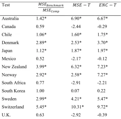
Table 1.10 shows the resulting forecast accuracy measures8. Based on the mean square error (MSE) ratio, we find evidence indicating that the composite model outperforms the benchmark model in predicting the movements of the US dollar for eight currencies. In addition, the MSE-T statistics are larger than the critical value in eight cases. Thus, we reject strongly the null of equal mean squared forecast errors indicating that the one-step-ahead forecast errors from the benchmark model are significantly larger than those from the composite model.
Finally, the ENC-T statistics are larger than the critical value in eight cases. This in turn suggests that the composite model contains added information for the US dollar exchange rate for eight currencies. Thus, the composite model encompasses the benchmark model in eight of the cases. Overall, these forecasting accuracy measures indicate that the price of oil enhances the predictability power of the monetary model of exchange rate.
Table 1.10 Forecasting Accuracy Measures. Test 𝑀𝑆𝐸𝐵𝑒𝑛𝑐ℎ𝑚𝑎𝑟𝑘 𝑀𝑆𝐸𝐶𝑜𝑚𝑝 𝑀𝑆𝐸 − 𝑇 𝐸𝑁𝐶 − 𝑇 Australia 1.42* 6.90* 6.67* Canada 0.59 -2.44 -0.29 Chile 1.06* 1.60* 1.75* Denmark 2.89* 2.53* 3.70* Japan 1.12* 1.87* 1.97* Mexico 0.52 -2.17 -0.12 New Zealand 3.99* 6.32* 7.23* Norway 2.92* 2.58* 7.27* South Africa 0.77 -2.91 -2.21 South Korea 1.00 0.07 0.22 Sweden 2.99* 4.21* 5.47* Switzerland 5.45* 10.31* 9.72* U.K. 0.63 -2.92 -0.39
* Indicates that the composite model is better in forecasting the USD.
1.6
Conclusion
The main objective of this paper is to investigate the impact of higher oil prices on the value of the USD against 13 major currencies, using quarterly data over the period 1986:Q1 through 2014:Q3. To meet this objective, we derived a flexible monetary model of the exchange rate containing the real price of crude oil.
Since our cointegration results indicate the existing of at least one cointegrating relationship between oil prices, monetary fundamentals, and the USD exchange rate, we estimated a vector error correction model and analyzed the effects of oil price movements on the USD exchange rate by computing impulse response functions.
We find evidence of a negative relationship between oil prices and the USD exchange rate. Furthermore, the forecast error variance decomposition analysis suggests that shocks to the real price of oil play a larger role in the movements of the USD exchange rate than do monetary fundamentals. We also find evidence suggesting an essential role of oil price in enhancing the forecasting power of the flexible monetary model of the exchange rate based on three measures of forecasting accuracy.
Chapter 2 - Oil Price Shocks and G7 Real Exchange Rates: The
Role of Monetary Policy
2.1
Introduction
In recent years, both oil prices and exchange rates have experienced sharp fluctuations, as shown in Figure 2.1 and 2.2. Swings in oil prices are transmitted to financi