AND
CHOQUET EXPECTED UTILITY
GILBERT W. BASSETT, JR., ROGER KOENKER, AND GREGORY KORDAS
Abstract. Recent developments in the theory of choice under uncertainty and risk yield a pessimistic decision theory that replaces the classical expected utility criterion with a Choquet expectation that accentuates the likelihood of the least favorable outcomes. A parallel theory has recently emerged in the literature on risk assessment. It is shown that pessimistic portfolio optimization based on the Choquet approach may be formulated as an exercise in quantile regression.
Algernon: I hope to-morrow will be a fine day, Lane.
Lane: It never is, sir.
Algernon: Lane, you’re a perfect pessimist.
Lane: I do my best to give satisfaction, sir.
Oscar Wilde, Importance of Being Earnest, Act I
1. Introduction
The cornerstone of the modern theory of decision making under risk is expected utility maximization as elaborated by Bernoulli (1738), Ramsey (1931), de Finetti (1937), von Neumann and Morgenstern (1944), Savage (1954), Fishburn (1982) and many subsequent authors. And yet there have been persistent doubts expressed about the adequacy of the expected utility framework to encompass the full range of human preferences over risky alternatives. Many variations on the the expected utility theme have been proposed, of these perhaps the most successful has been the family of non-additive, or dual, or rank-dependent formulations of Schmeidler (1989), Yaari Version January 8, 2004. The research was partially supported grant SES-99-11184. The authors would like to thank Quanshui Zhao and Steve Portnoy for helpful discussions related to this work. They would also like to express their appreciation to seminar participants at Toronto, U. Penn Warwick, UCL and EUI-Florence.
(1987), and Quiggin (1982). The familiar Lebesgue integral of the expected utility computation is replaced by a Choquet integral, thereby permitting, for example, the probability weights associated with the least favorable outcomes to be accentuated and thereby yielding a pessimistic decision criterion.
Our aim in this paper is to provide an elementary exposition of one variant of the Choquet expected utility theory as it applies to decisions under risk, to link this the-ory with some recent developments in the literature on risk assessment, and finally to describe its application to the problem of portfolio choice. The problem of portfolio allocation is central to economic decision theory and thus constitutes an acid test of any new criterion designed to evaluate risky alternatives. By offering a general approach to portfolio allocation for pessimistic Choquet preferences we hope to en-courage a critical reexamination of the role of attitudes toward risk in this important setting. In contrast to conventional mean-variance portfolio analysis implemented by solving least squares problems, pessimistic portfolios will be constructed by solving quantile regression problems. Our results complement recent work in the financial econometrics literature on estimation and inference in conditional quantile models, as e.g. in Engle and Manganelli (2001), Bouy´e and Salmon (2002), Christoffersen and Diebold (2003), and Linton and Whang (2003).
2. Choquet Expected Utility
Consider the problem of choosing between two real-valued random variables, X
and Y, having distribution functions, F and G, respectively. Comparing expected utilities, we prefer X toY if EFu(X) = Z ∞ −∞ u(x)dF(x)> Z ∞ −∞ u(x)dG(x) =EGu(Y)
In this framework, the utility function, u, bears the entire burden of representing the decision makers’ attitudes toward risk. Changing variables, we have the equivalent formulation that X is preferred toY if
(2.1) EFu(X) = Z 1 0 u(F−1(t))dt > Z 1 0 u(G−1(t))dt =EGu(Y),
in effect, we have transformed the original integrand into “equally likely” slices on the interval [0,1], now integrable with respect to Lebesgue measure. This formulation of expected utility in terms of the quantile functions F−1(t) of X and G−1(t) of Y is
In its simplest form Choquet expected utility introduces the possibility that pref-erences may require a distortion of the original probability assessments, rather than integrating dt we are permitted to integrate, dν(t), with respect to some other prob-ability measure defined on the interval [0,1]. Preferences are thus represented by a pair of functions (u, ν): u transforms (monetary) outcomes into utility terms, while
ν transforms probability assessments.1 Now X is preferred to Y if (2.2) Eν,Fu(X) = Z 1 0 u(F−1(t))dν(t)> Z 1 0 u(G−1(t))dν(t) =Eν,Gu(Y).
Since our change of variables has ordered the events, u(F−1
(t)) andu(G−1
(t)) are also ordered according to increasing desirability. We assume throughout that u is mono-tone increasing. The distortion function ν acts to inflate or deflate the probabilities
according to the rank ordering of the outcomes. The distortion may systematically increase the implicit likelihood of the least favorable events, for example. But, unlike the original form of the prospect theory of Kahneman and Tversky (1979), it cannot systematically distort small probabilities per se. In contrast, cumulative prospect theory, as developed by Tversky and Kahneman (1992) and Wakker and Tversky (1993), is quite closely aligned with the Choquet approach.
Admittedly, there is something mildly schizophrenic about decision makers who accept at face value probabilities represented by the distribution functions F and G, and then intentionally distort these probabilities in the process of turning them into actions. More general forms of Choquet expected utility, following Schmeidler (1989), dispense entirely with initial probabilities. Monotone set functions, or Choquet ca-pacities, are employed to assign nonadditive probabilities directly to events, enabling the theory to address distinctions between risk, uncertainty and ambiguity that have played a prominent role in the recent literature. By restricting attention to settings in which the Choquet capacity is expressed as the composition of an increasing function
ν : [0,1] → [0,1] with ν(0) = 0 and ν(1) = 1, and a probability measure we sacri-fice some of the power and elegance of the general theory, but in return we obtain a very concise representation of preferences in terms of a pair of simple and easily interpretable functions (u, ν). Following Yaari (1987), we will focus our attention on the function ν, first interpreting it in terms of the possible optimism or pessimism
1Whether this latter transformation is a matter of “perception” or “attitude” or some other
category of psychological experience has been a matter of some debate. We prefer Yaari’s assertion that the theory describes “how perceived risk is processed into choice.”
of the decision maker, then briefly describing its axiomatic underpinnings.2 A brief
exposition of the interrelationship between various forms of the Choquet expectation is provided in an Appendix.
2.1. Pessimism. Choquet expected utility leads naturally to an interpretation of the distorting probability measure ν as a reflection of optimism or pessimism. If the distortion function, ν, is concave, then the least favorable events receive increased weight and the most favorable events are discounted reflecting pessimism. To see this, it may be helpful to consider the case that ν is absolutely continuous as well as concave and therefore has a decreasing density with respect to Lebesgue measure. Thus, instead of the uniform weighting implicit in the expected utility criterion, the Choquet criterion accentuates the weight of the least favorable events and reduces the weight assigned to the most favorable events. When ν is convex the situation is reversed, optimism prevails, and the Choquet integral exaggerates the likelihood of the more favorable events and downplays the likelihood of the worst outcomes. As noted already by Quiggin (1982) and Schmeidler (1989), distortion functions that are initially concave and then convex offer an alternative to the classical Friedman and Savage (1948) rationale for the widespread, but still puzzling, observation that many people seem to be willing to buy insurance and gamble at (nearly) the same time.3
The simplest distortions are those given by the one parameter family, να(t) =
min{t/α,1} forα ∈[0,1]. In this case, we have,
Eναu(X) =α
−1
Z α
0
u(F−1(t))dt,
and we see that – relative to the usual computation of expected utility – the prob-abilities of the α least favorable outcomes are inflated and the 1−α proportion of most favorable outcomes are discounted entirely. This family will play an important role as a building block for more general distortion functions in the sequel.
2Wakker (1990) has shown that Schmeidler’s general theory of Choquet preferences coincides with
the rank dependent, or anticipated utility, formulations of Quiggin and Yaari for decision making under risk, that is when choices are over given probability distributions.
3Whether optimism and pessimism will eventually find a legitimate place in formal decision theory
is likely to remain somewhat controversial – it seems advisable to recall that Savage (1954, p. 68) did not seem think that they could be acommodated into his view of subjective expected utility. But given the long-standing dissatisfaction with expected utility theory it is surely worthwhile to continue to explore the implications of alternative schemes particularly when they are sufficiently tractable to yield concrete competing predictions about behavior for problems of real economic significance.
2.2. Axiomatics. Recall that if A denotes a mixture space of “acts” consisting of functions mapping states of nature,Sto a set of probability distributions on outcomes, then the von Neumann Morgenstern axioms impose the following condition on the binary preference relation () over A:
(A) (Independence) For all f, g, h∈ A and α ∈ (0,1), then f g implies αf + (1−α)hαg+ (1−α)h,
Schmeidler’s seminal 1989 paper argues that the independence axiom “may be too powerful to be acceptable”, and he proposes a weaker form of independence:
(A0
) (Comonotonic Independence) For all pairwise comonotonic acts f, g, h ∈ A
and α∈(0,1), then f g implies αf+ (1−α)hαg+ (1−α)h,
Comonotonicity, a concept introduced by Schmeidler, plays a pivotal role.
Definition 1. Two acts f and g in A are are comonotonic if for no s and t in S, f(s)f(t) and g(t)g(s).
By restricting the applicability of the independence axiom only to comonotonic acts, the force of the axiom is considerably weakened. Schmeidler (1986, 1989) shows that the effect of replacing (A) by (A0
) is precisely to enlarge the scope of preferences from those representable by a von Neumann-Morgenstern (Savage) utility function, u, to those representable by a pair, (u, ν), consisting of a utility function and a Choquet capacity.
To clarify the role of comonotonicity it is useful to consider the following reformu-lation of the definition in terms of random variables.
Definition 2. Two random variables X, Y : Ω → R are comonotonic if there exists a third random variable Z : Ω → R and increasing functions f and g such that X =f(Z) and Y =g(Z).
In the language of classical rank correlation, comonotonic random variables are perfectly concordant, i.e. have rank correlation 1. The classical Fr´echet bounds for the joint distribution function,H, of two random variables, XandY, with univariate marginals F and G is given by
max{0, F(x) +G(y)−1} ≤H(x, y)≤min{F(x), G(y)}
Comonotonic X and Y achieve the upper bound.
From our point of view a crucial property of comonotonic random variables is the behavior of the quantile functions of their sums. For comonotonic random variables
X, Y, we have FX−+1Y(u) =F −1 X (u) +F −1 Y (u)
This is because, by comonotonicity we have a U ∼ U[0,1] such that Z = g(U) =
F−1
X (U)+F
−1
Y (U) wheregis left continuous and increasing, so by monotone invariance
of the quantile function we have, Fg−(U1)=g◦FU−1 =F−1
X +F
−1
Y .
This property will play an essential role in our formulation of pessimistic portfolio theory, a topic that we will introduce with a brief review of some closely related recent work in the theory of risk assessment.
3. Measuring Risk
Motivated by regulatory concerns in the financial sector there has been considerable recent interest in the question of how to measure portfolio risk. An influential paper in this literature is Artzner, Delbaen, Eber, and Heath (1999), which provides an axiomatic foundation for “coherent” risk measures.
Definition 3. (Artzner et al) For real valued random variables X ∈ X on (Ω,A) a mapping %:X →R is called a coherent risk measure if it is:
(i) Monotone: X, Y ∈ X,withX ≤Y ⇒%(X)≥%(Y).
(ii) Subadditive: X, Y, X+Y ∈ X, ⇒%(X+Y)≤%(X) +%(Y).
(iii) Linearly Homogeneous: For all λ≥0 and X ∈ X, %(λX) =λ%(X).
(iv) Translation Invariant: For all λ∈R and X ∈ X, %(λ+X) =%(X)−λ.
These requirements rule out many of the conventional measures of risk traditionally used in finance. In particular, measures based on second moments are ruled out by the monotonicity requirement, and quantile based measures like the value-at-risk are ruled out by subadditivity. A measure of risk that is coherent and that has gained considerable recent prominence in the wake of these findings is,
%να(X) =− Z 1 0 F−1(t)dν(t) =−α−1 Z α 0 F−1(t)dt,
where ν(t) = min{t/α,1} as in Section 2. Variants of %να(X) have been suggested
under a variety of names, including expected shortfall (Acerbi and Tasche (2002)), conditional value at risk (Rockafellar and Uryasev (2000)), tail conditional expecta-tion (Artzner, Delbaen, Eber, and Heath (1999)). For the sake of brevity we will call
%να(X) the α-risk of the random prospect X. Clearly, α-risk is simply the negative
Having defined α-risk in this way, it is natural to consider the criteria: %να(X)− λµ(X), orµ(X)−λ%να(X).Minimizing the former criterion may be viewed as
minimiz-ing risk subject to a constraint on mean return; maximizminimiz-ing the latter criterion may be viewed as maximizing return subject to a constraint on α-risk. Several authors, including Denneberg (1990), Rockafellar and Uryasev (2000), Jaschke and K¨uchler (2001), and Ruszczyski and Vanderbei (2003), have suggested criteria of this form as alternatives to the classical Markowitz criteria in which α-risk is replaced by the standard deviation of the random variable X. Since µ(X) = R F−1
X (t)dt = −%1(X)
these criteria are special cases of the following more general class.
Definition 4. A risk measure % is pessimistic if, for some probability measure ϕ on
[0,1],
%(X) =
Z 1 0
%να(X)dϕ(α).
To see why such risk measures should be viewed as pessimistic, note that by the Fubini Theorem we can write,
%(X) =− Z 1 0 α−1 Z α 0 F−1(t)dtdϕ(α) =− Z 1 0 F−1(t) Z 1 t α−1dϕ(α)dt.
In the simplest case, we can take ϕ as a finite sum of (Dirac) point masses, say
dϕ=Pmi=0ϕiδτi with ϕi ≥0,
P
ϕi = 1, and 0 =τ0 < τ1 < ... < τm ≤1. Noting that Z 1 t α−1δ τ(α)dα=τ −1I(t < τ), we can write (3.1) %(X) = Z 1 0 %να(X)dϕ(α) =−ϕ0F −1(0)− Z 1 0 F−1(t)γ(t)dt whereγ(t) = Pmi=1ϕiτ −1
i I(t < τi). Positivity of the point masses, ϕi, assures that the
resulting density weights are decreasing, so the resulting distortion in probabilities acts to accentuate the implicit likelihood of the least favorable outcomes, and depress the likelihood of the most favorable ones. Such preferences are clearly “pessimistic”. We may interpret the α-risks, %α(·) as the extreme points of the convex set of
coherent risk measures, and this leads to a nice characterization result. Following Kusuoka (2001) we will impose some additional regularity conditions on %:
Definition 5. Let L∞
denote the space of all bounded real-valued random variables on (Ω,F,P) with P non-atomic. A map %:L∞
(i.) % is law invariant, i.e. %(X) =%(Y) if X, Y ∈ L∞
have the same probability law.
(ii.) %is comonotonically additive, i.e. X, Y ∈ L∞
comonotone implies that%(X+
Y) =%(X) +%(Y).
The first condition requires only that % depend upon observable properties of its argument. Random variables with the same distribution functions should have the same risk. The second condition refines slightly the subadditivity property: subad-ditivity becomes adsubad-ditivity when X and Y are comonotone. We can now succinctly reformulate the characterization result of Kusuoka (2001) and Tasche (2002).
Theorem 1. A regular risk measure is coherent if and only if it is pessimistic.
This result justifies our earlier comment that the elementary α-risks are funda-mental building blocks: any concave distortion function, ν, can be approximated by a piecewise linear concave function. These linear approximants are nothing but the weighted sums of Dirac’s introduced above. They correspond to risk functions of the form (3.1) with γ(t) =Pmi=1ϕiτ
−1
i I(t < τi) piecewise constant and decreasing. Note
that as a special case such ν’s are entitled to place positive weight ϕ0 on the least favorable outcome, so they include the extreme case of maximin preferences.
4. Pessimistic Portfolio Allocation
We have seen that decision making based on minimizing a “coherent” measure of risk as defined by Artzner, Delbaen, Eber, and Heath (1999) is equivalent to Choquet expected utility maximization using a linear form of the utility function. But the question remains: Does the Choquet approach to decision making under risk lead to tractable methods for analyzing complex decision problems of practical importance? An affirmative answer to this question is provided in this section.
4.1. Onα-risk as Quantile Regression. Empirical strategies for minimizingα-risk lead immediately to the methods of quantile regression. Let
ρα(u) =u(α−I(u <0))
denote the piecewise linear (quantile) loss function and consider the problem, min
ξ∈R Eρα(X−ξ).
It is well known, e.g. Ferguson (1967), that any ξ solving this problem is an αth quantile of the random variable X. Evaluating at a minimizer, ξα we find that
minimizing the usual α-quantile objective function is equivalent to evaluating the sum of expected return and the α-risk of X, and then multiplying byα.
Theorem 2. Let X be a real-valued random variable with EX=µ <∞, then
min
ξ∈R Eρα(X−ξ) = α(µ+%να(X)).
Proof: Noting that,
Eρα(X−ξ) =α(µ−ξ)− Z ξ −∞ (x−ξ)dFX(x), is minimized when ξα=F −1 X (α), we have, Eρα(X−ξα) =αµ− Z α 0 F−1(t)dt =αµ+α% να(X).
This result provides a critical link to the algorithmic formulation developed in the next subsection.
4.2. How to be Pessimistic. Given a random sample {xi : i = 1, ..., n} on X, an
empirical analogue of α-risk can thus be formulated as (4.1) %ˆνα(x) = (nα) −1min ξ∈R n X i=1 ρα(xi−ξ)−µˆn
where ˆµn denotes an estimator of EX = µ, presumably, ¯xn. The advantage of the
optimization formulation becomes apparent as soon as we begin to consider portfolios. LetY =X>
πdenote a portfolio of assets comprised ofX = (X1, ..., Xp)>with
port-folio weights π. Suppose now that we observe a random sample {xi = (xi1, ..., xip) :
i = 1, ..., n} from the joint distribution of asset returns, and we wish to consider portfolios minimizing
(4.2) min
π %να(Y)−λµ(Y).
This is evidently equivalent to simply minimizing %να(Y) subject to a constraint on
mean return. Alternatively, we could consider maximizing mean return subject to a constraint on α-risk; this equivalent formulation might be interpreted as imposing a regulatory constraint on a risk neutral agent. Since µ(Y) =−%ν1(Y), the mean is also just another α-risk, so the problem (4.2) may be viewed as a special discrete example of the pessimistic risk measures of Definition 4. More general forms are introduced in Section 4.4.
We will impose the additional constraint that the portfolio weights π sum to one, and reformulate the problem as,
min π %να(X > π)s.t. µ(X> π) = µ0, 1> π= 1.
Taking the first asset as numeraire we can write the sample analogue of this problem as (4.3) min (β,ξ)∈Rp n X i=1 ρα(xi1− p X j=2 (xi1−xij)βj−ξ)s.t.x¯ > π(β) =µ0,
where π(β) = (1−Ppj=2βj, β>)>. Note that the term ˆµn in (4.1) can be neglected
since the mean is constrained to take the value µ0, and the factor (nα)−1 can be
absorbed into the Lagrange multiplier of the mean return constraint. This is a linear programming problem of the type consider by Koenker and Bassett (1978), and can be solved very efficiently even when n and p are large by interior point methods. It is easy to verify that the solution is invariant to the choice of the numeraire asset. At the solution, ˆξ is an αth sample quantile of the chosen portfolio’s (in-sample) returns distribution. The required mean return constraint implicitly corresponds to a particular choice of λ in the original specification (4.2). Note that we have not (yet) imposed any further constraints on the portfolio weights β, but given the linear programming form of the problem (4.3) it is straightforward to do so. Software to compute solutions to the problems (5.2-4) subject to arbitrary linear inequality con-straints, and written for the public domain dialect, R, of the S language of Chambers (1998), is available from the authors on request. The algorithms used are based on the interior point, log-barrier methods described in Portnoy and Koenker (1997).
The problem posed in (4.3) is (almost) a conventional quantile regression problem. The only minor idiosyncrasy is the mean return constraint, but it is easy to impose this constraint by simply adding a single pseudo observation to the sample consisting of response κ(¯x1−µ0) and design row κ(0,x1¯ −x2, ...,¯ x1¯ −x¯p)>. (The zero element
corresponds to the intercept column of the design matrix.) For sufficiently large κwe are assured that the constraint will be satisfied. Varying µ0 we obtain an empirical α-risk frontier analogous to the Markowitz mean-variance frontier.
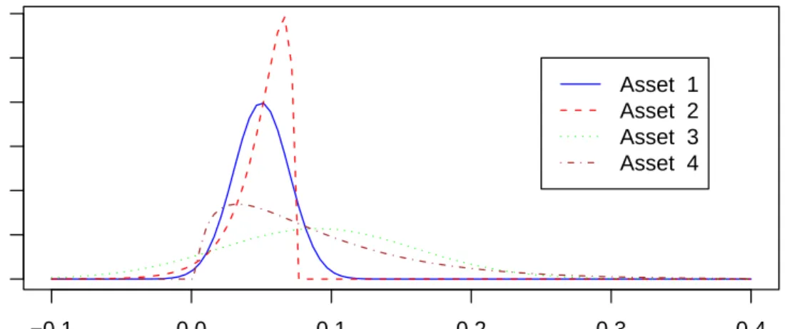
4.3. An Example. Consider forming portfolios from four independently distributed assets with marginal returns densities illustrated in Figure 1. Asset 1 is normally distributed with mean 0.05 and standard deviation 0.02. Asset 2 has a reversed χ2 3
−0.1 0.0 0.1 0.2 0.3 0.4 0 5 10 15 20 25 30 return density Asset 1 Asset 2 Asset 3 Asset 4
Figure 1. Four Asset Densities
those of asset 1. Similarly, assets 3 and 4 are constructed to have identical means (0.09) and standard deviations (0.07). But for the second pair of densities theχ2
3asset
is skewed to the right, as usual, not to the left. The example is obviously chosen with malice aforethought. Asset 2 is unattractive relative to its twin, asset 1, having worse performance in both tails. And asset 3 is unattractive relative to asset 4 in both tails. But from a mean-variance viewpoint the two pairs of assets are indistinguishable.
To compare portfolio choices we generate a sample of n = 1000 observations from the returns distribution of the four assets. We then estimate optimal mean variance portfolio weights by solving
(4.4) min (β,ξ)∈Rp n X i=1 (xi1− p X j=2 (xi1−xij)βj−ξ)2 s.t.x¯ > π(β) =µ0, where π(β) = (1 − Ppj=2βj, β > )>
. We choose µ0 = 0.07, and obtain π( ˆβ) = (0.271,0.229,0.252,0.248). We then estimate optimal α-risk portfolio weights for
α = .1 by solving (4.3) again with required mean return of µ0 = 0.07, obtaining
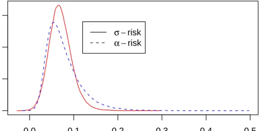
0.0 0.1 0.2 0.3 0 5 10 15 return density σ −risk α −risk
Figure 2. Markowitz (σ-risk) vs. Choquet (α-risk) portfolio returns densities: Portfolios are constrained to achieve the same in-sample mean return; note that the Choquet portfolio has better performance than the Markowitz portfolio in both the lower and upper tails.
“attractive” assets 1 and 4, and less to assets 2 and 3, compared to the mean variance portfolio.
To evaluate our two portfolio allocations we generate a new sample ofn = 100,000 observations for the four assets, and we plot estimated densities of the two portfolios returns in the left panel of Figure 2. It is apparent that the α-risk portfolio has better performance than the mean-variance (σ-risk) portfolioin both tails. It is safer in the lower tail, and also more successful in the upper tail. Improved performance in the lower tail should be expected from the Choquet portfolio since it is explicitly designed to maximize the expected return from the α least favorable outcomes. Improved performance in the upper tail may be attributed to the inability of the variance to distinguish upside from downside risk, and thus its desire to avoid both. The Choquet portfolio exhibits no such tendency. Risk is entirely associated with the behavior in
0.0 0.1 0.2 0.3 0.4 0.5 0 5 10 15 return density σ −risk α −risk
Figure 3. Markowitz (σ-risk) vs. Choquet (α-risk) portfolio returns densities: Portfolios are constrained to achieve the same in-sample α -risk; so performance in the lower tail is virtually identical, but the Cho-quet portfolio now has much better performance than the Markowitz portfolio in the upper tail.
the lower tail, and the expected return component of the objective function is able to exploit whatever opportunities exist in the upper tail.
The foregoing comparison is strongly conditioned by the requirement that the means of the two portfolios are identical. Our second comparison keeps the same
σ-risk portfolio, but chooses theα-risk portfolio to maximize expected return subject to achieving the same α-risk as that achieved by the σ-risk portfolio. This yields a new α-risk portfolio with weights π( ˆβ) = (0.211,0.119,0.144,0.526) that places even more weight on asset 4 and thereby achieves a mean return (in the initial sample) of 0.768. We plot the estimated returns densities of the two portfolios based on the
tail (with α= 0.1) we are able to achieve considerably better (68 basis points!) per-formance. Of course the variance and standard deviation of the new α-risk portfolio is larger than for its σ-risk counterpart, but this is attributable to its better perfor-mance in the upper tail, a result that underscores the highly unsatisfactory nature of second moment information as a measure of risk in asymmetric settings.
4.4. Portfolio Allocation for General Pessimistic Preferences. Although the
α-risks provide a convenient one-parameter family of coherent risk measures, they are obviously rather simplistic. As we have already suggested, it is natural to consider weighted averages of α-risks:
%ν(X) = m X
k=1
νk%ναk(X).
Where the weights, νk:k = 1, ..., m, are positive and sum to one. These general risk
criteria can also be easily implemented empirically extending the formulation in (4.3)
(4.5) min (β,ξ)∈Rp+m m X k=1 n X i=1 νkρα(xi1− p X j=2 (xi1−xij)βj −ξk)s.t.x¯ > π(β) =µ0.
The only new wrinkle is the appearance of m distinct intercept parameters repre-senting the m estimated quantiles of the returns distribution of the chosen portfolio. In effect we have simply stacked m distinct quantile regression problems on top of one another and introduced a distinct intercept parameter for each of them, while constraining the portfolio weights to be the same for each quantile. Since the νk are
all positive, they may be passed inside the ρα function to rescale the argument. The
asymptotic behavior of such constrained quantile regression estimators is discussed in Koenker (1984). Since any pessimistic distortion function can be represented by a piecewise linear concave function generated as a weighted average of α-risks this approach offers a general solution to the problem of estimating pessimistic portfolio weights.
5. Conclusion
Expected utility theory and mean-variance portfolio allocation are firmly embedded in the foundations of modern decision theory and have withstood more than a half century of criticism. Whether a generally accepted alternative theory can be built on the foundations of Choquet expectated utility remains an open question. But it is a question that we believe deserves further investigation.
We have shown that a general form of pessimistic Choquet preferences under risk with linear utility leads to optimal portfolio allocation problems that can be solved by quantile regression methods. These portfolios may also be interpreted as maximiz-ing expected return subject to a “coherent” measure of risk in the sense of Artzner, Delbaen, Eber, and Heath (1999). By providing a general method for computing pessimistic portfolios based on Choquet expected returns we hope to counter the impression occassionally seen in the literature that alternatives to the dominant ex-pected utility view are either too vague or too esoteric to be applicable in problems of practical significance. There is a growing body of scholarship suggesting that pes-simistic attitudes toward risk offer a valuable complement to conventional views of risk aversion based on expected utility maximization; portfolio allocation would seem to provide a valuable testing ground for further evaluation of these issues.
Appendix A. Choquet Capacities and the Choquet Integral Since our formulation of Choquet expected utility in terms of quantile functions is somewhat less conventional than equivalent expressions formulated in terms of distribution functions, it is perhaps worthwhile to briefly describe the connection between the two formulations.
Let X be a real-valued random variable on Ω with an associated system of of sets, or “events”, A. A Choquet capacity, or non-additive measure,µonA, is a monotone set function (forA, B∈ A, A ⊆ B implies that µ(A) ≤ µ(B)), normalized so that µ(∅) = 0 and µ(Ω) = 1. The Choquet expectation ofX, with respect to a capacityµ, is given by,
EµX= Z Xdµ= Z 0 −∞ (µ({X > x})−1)dx+ Z ∞ 0 µ({X > x})dx
In this form, with µdefined directly on events, there is no necessity for any intermediate evaluation of probabilities. The Choquet expectation can accommodate various notions of ambiguity, or uncer-tainty, arising, for example, in the well-known examples of Ellsberg (1961). If, on the other hand,X is assumed to possess a distribution function F, and therefore a survival function, ¯F(x) = 1−F(x) we may write, µ({X > x}) = Γ( ¯F(x)), for some monotone function Γ such that Γ(0) = 0 and Γ(1) = 1. The Choquet expectation becomes,
EµX = Z 0 −∞ (Γ( ¯F(x))−1)dx+ Z ∞ 0 Γ( ¯F(x))dx.
In the special case that µ is Lebesgue measure, Γ is the identity and we have the well-known expression, EX=− Z 0 −∞ F(x)dx+ Z ∞ 0 (1−F(x))dx.
If Γ is absolutely continuous with densityγ, we can integrate by parts to obtain,
EµX= Z ∞ −∞ xdΓ( ¯F(x)) =− Z ∞ −∞ xγ( ¯F(x))dF(x),
Finally, changing variables,x→F−1 (t), we have EµX =− Z 1 0 F−1 (t)γ(1−t)dt = Z 1 0 F−1 (1−s)γ(s)ds = Z 1 0 F−1 (1−s)dΓ(s).
The last expression reveals another slightly mysterious aspect of the conventions used in defining the Choquet capacity. The distortion Γ as defined above integrates the quantile function backwards. Thus following the conventions of Section 2, if we would like to define a distortionν such that
Z 1 0 F−1 (s)dν(s) = Z 1 0 F−1 (1−s)dΓ(s).
then clearly we must haveν(s) =−Γ(1−s). Consequently, if Γ is convex, then ν will be concave, and vice versa. It is for this reason that pessimism, and uncertainty aversion, are often identified with convex capacities, as for example in Schmeidler (1989).
References
Acerbi, C.,andD. Tasche(2002): “Expected Shortfall: A Natural coherent alternative to Value at Risk,”Economic Notes, 31, 379–388.
Artzner, P., F. Delbaen, J.-M. Eber, and D. Heath(1999): “Coherent Measures of Risk,”
Math. Finance, 9, 203–228.
Bernoulli, D. (1738): “Specimen theoriae novae de mensura sortis,” Commentarii Academiae Scientiarum Imperialis Petropolitanae, 5, 175–192, translated by L. Sommer inEconometrica, 22, 23-36.
Bouy´e,and M. Salmon(2002): “Dynamic Copula Quantile Regressions and Tail Area Dynamic Dependence in Forex Markets,” preprint.
Chambers, J. M.(1998): Programming with Data: A Guide to the S Language. Springer.
Christoffersen, P., and F. Diebold (2003): “iFinancial asset returns, direction-of-change forecasting, and volatility dynamics,” preprint.
de Finetti, B.(1937): “La pr´evision ses lois logiques, ses sources subjectives,”Annals de l’Instutute Henri Poincar´e, 7, 1–68, translated by H.E. Kyburg in Studies in Subjective Probability, H.E. Kyburg and H.E. Smokler, (eds.), Wiley, 1964.
Denneberg, D. (1990): “Premium Calculation: Why standard deviation should be replaced by absolute deviation,”ASTIN Bulletin, 20, 181–190.
Engle, R., and S. Manganelli (2001): “CAViaR: Conditional autoregressive value at risk by regression quantiles,” preprint.
Ferguson, T. S. (1967): Mathematical Statistics: A Decision Theoretic Approach. iAcademic Press.
Friedman, M., andL. Savage(1948): “The utility analysis of choices involving risk,”J. Political Economy, 56, 279–304.
Jaschke, S.,andU. K¨uchler(2001): “Coherent Risk Measure and Good Deal Bounds,”Finance and Stochastics, 5, 181–200.
Kahneman, D., and A. Tversky(1979): “Prospect theory: An analysis of decision under risk,”
Econometrica, 47, 263–291.
Koenker, R. (1984): “A Note on L-estimators for Linear Models,”Stat and Prob Letters, 2, 323– 325.
Koenker, R., and G. Bassett(1978): “Regression Quantiles,”Econometrica, 46, 33–50.
Kusuoka, S. (2001): “On Law Invariant Coherent Risk Measures,”Advances in Math. Econ., 3, 83–95.
Linton, O., and Y.-J. Whang (2003): “A quantilogram approach to evaluating directional predictability,” preprint.
Portnoy, S., and R. Koenker(1997): “The Gaussian Hare and the Laplacian Tortoise: Com-putability of Squared-error Versus Absolute-error Estimators,”Statistical Science, 12, 299–300.
Quiggin, J.(1982): “A Theory of Anticipated Utility,”J. of Econ. Behavior and Organization, 3, 225–243.
Ramsey, F.(1931): “Truth and Probability,” inThe Foundations of Mathematics and Other Logical Essays. Harcourt Brace.
Rockafellar, R., and S. Uryasev (2000): “Optimization of conditional VaR,” J. of Risk, 2, 21–41.
Ruszczyski, A.,andR. Vanderbei(2003): “Frontiers of stochastically nondominated portfolios,”
Econometrica, 7, 1287–1298.
Savage, L.(1954): Foundations of Statistics. Wiley.
Schmeidler, D. (1986): “Integral representation without additivity,” Proceedings of Am Math Society, 97, 255–261.
(1989): “Subjective Probability and Expected Utility without Additivity,”Econometrica, 57, 571–587.
Tasche, D. (2002): “Expected Shortfall and Beyond,”Journal of Banking and Finance, 26, 1519– 1533.
Tversky, A.,and D. Kahneman(1992): “Advances in Prospect Theory: Cumulative Represen-tation of Uncertainty,”J. Risk and Uncertainty, 5, 297–323.
von Neumann, J., and O. Morgenstern (1944): Theory of Games and Economic Behavior. Princeton.
Wakker, P. (1990): “Under Stochastic Dominance Choquet-Expected Utility and Anticipated Utility are Identical,”Theory and Decision, 29, 119–132.
Wakker, P.,and A. Tversky (1993): “An Axiomatization of Cumulative Prospect Theory,”J. Risk and Uncertainty, 7, 147–176.
University of Illinois at Chicago
University of Illinois at Urbana-Champaign