Revised parameter estimation methods for the Pitman monthly rainfall-runoff model

(1)

REVISED PARAMETER ESTIMATION METHODS FOR

THE PITMAN MONTHLY RAINFALL-RUNOFF MODEL

A thesis submitted in fulfilment of the requirements for the degree of

Master of Science of Rhodes University Grahamstown South Africa By Evison Kapangaziwiri October 2007

(2)

Dedication

This thesis is dedicated to my friend and wife, Concillia, and our son Hanyadzashe who had patiently endured my long absence from home. Thank you guys for all your understanding and support. Love ya!

(3)

Acknowledgements

I am grateful to Prof Denis Hughes, my supervisor, for the support and guidance throughout the conception and execution of this research work. I am especially thankful for his patience in going through the numerous manuscripts that preceded this final report. The equations developed for the estimation procedures were packaged into a small and neat computer program which he coded for me. Thank you also to David Forsyth for assisting with the conversion of data to formats acceptable in the SPATSIM software. A number of small programs were written for my benefit and this is greatly appreciated.

A special word of thanks goes out to the providers of data used in the development and testing of the estimation methods in this thesis, Department of Water Affairs and Forestry (DWAF), the Zimbabwe National Water Authority (ZINWA), Dr Rikard Liden of SWECO Consultants (Sweden), Mr. Anthony Mporokoso of Department of Water Affairs (Zambia). I also would like to express my gratitude to numerous colleagues who help shape this thesis through constructive comments and encouragement.

I would like to thank Institute for Water Research (IWR) for their financial support in the form of bursary for 2006 and a partial bursary for 2007. The financial assistance of the department of Labour (DST) towards this research is also hereby acknowledged. Opinions expressed and conclusions arrived at, are those of the author and are not necessarily to be attributed to the DST or IWR.

I would like to thank all members of staff of the Institute for Water Research for various fruitful and enlightening discussions that helped my appreciation of various water related issues.

(4)

ABSTRACT

In recent years, increased demands have been placed on hydrologists to find the

most effective methods of making predictions of hydrologic variables in ungauged

basins. A huge part of the southern African region is ungauged and, in gauged

basins, the extent to which observed flows represent natural flows is unknown,

given unquantified upstream activities. The need to exploit water resources for

social and economic development, considered in the light of water scarcity

forecasts for the region, makes the reliable quantification of water resources a

priority.

Contemporary approaches to the problem of hydrological prediction in ungauged

basins in the region have relied heavily on calibration against a limited gauged

streamflow database and somewhat subjective parameter regionalizations using

areas of assumed hydrological similarity. The reliance of these approaches on

limited historical records, often of dubious quality, introduces uncertainty in water

resources decisions. Thus, it is necessary to develop methods of estimating model

parameters that are less reliant on calibration.

This thesis addresses the question of whether physical basin properties and the

role they play in runoff generation processes can be used directly in the

estimation of parameter values of the Pitman monthly rainfall-runoff model. A

physically-based approach to estimating the soil moisture accounting and runoff

parameters of a conceptual, monthly time-step rainfall-runoff model is proposed.

The study investigates the physical meaning of the model parameters, establishes

linkages between parameter values and basin physical properties and develops

relationships and equations for estimating the parameters taking into account the

(5)

methods are then tested in selected gauged basins in southern Africa and the

results of model simulations evaluated against historical observed flows.

The results of 71 basins chosen from the southern African region suggest that it is

possible to directly estimate hydrologically relevant parameters for the Pitman

model from physical basin attributes. For South Africa, the statistical and visual fit

of the simulations using the revised parameters were at least as good as the

current regional sets, albeit the parameter sets being different. In the other

countries where no regionalized parameter sets currently exist, simulations were

equally good.

The availability, within the southern African region, of the appropriate physical

basin data and the disparities in the spatial scales and the levels of detail of the

data currently available were identified as potential sources of uncertainty. GIS

and remote sensing technologies and a widespread use of this revised approach

(6)

2 RAINFALL-RUNOFF MODELLING ... 8

2.1 Introduction ... 8

2.2 Model types and structure ... 9

2.3 Parameter interaction and sensitivity ... 14

2.4 Model parameter calibration and validation ... 17

2.4.1 Model Calibration... 17

2.4.2 Parameter validation... 20

2.4.3 Assessment of model performance... 21

2.5 Modelling in ungauged basins ... 24

2.5.1 The Ungauged Problem ... 24

2.5.2 Parameter Regionalization ... 25

2.6 Parameter uncertainty in hydrological modelling ... 29

2.7 Use of hydrological models in southern Africa... 30

3 THE PITMAN MODEL... 33

3.2 The Pitman model ... 33

3.3 Use of the Pitman model in SPATSIM ... 37

4 PITMAN MODEL PARAMETER DESCRIPTIONS ... 41

4.1.1 Seasonal variations... 42

4.1.2 Scale effects ... 42

4.2 Rainfall Distribution Factor (RDF) ... 42

4.3 Interception Parameters: PI1, PI2 ... 44

4.4 Infiltration Parameters: AI, ZMIN, ZAVE, ZMAX ... 47

4.5 Soil Moisture Storage Parameters: ST, SL... 51

4.6 Soil Moisture Runoff Parameters: FT, POW... 55

4.7 Groundwater Recharge Parameters: SL, GW,GPOW... 57

4.8 Evaporation Parameters: R, AFOR, FF ... 59

4.9 Runoff Routing Parameters: TL, GL, CL ... 61

4.10 Groundwater Accounting Parameters: DDENS, T, S, RWL, GWSlope, RipFactor ... 63

4.11 Channel Loss Parameter: TLGMax... 70

4.12 Non-Natural Parameters ... 74

4.12.1 Water Use Parameters: Airr, IWR, IrrAreaDmd, NIrrDmd, EffRf.... 74

4.12.2 Reservoir Parameters: DAREA, MAXDAM, A, B ... 78

(7)

5 PARAMETER ESTIMATION METHODS FOR THE PITMAN MODEL ... 82

5.2 Soil moisture accounting, subsurface runoff and recharge parameters .... 85

5.2.1 Estimating STsoil... 85

5.2.2 Estimating STunsat... 87

5.2.3 Estimating FTsoil... 90

5.2.4 Estimating FTunsat... 92

5.2.5 Estimating POW ... 93

5.2.6 Estimating GW and GPOW ... 97

5.3 Soil surface infiltration parameters ... 98

5.3.1 Generating runoff using the infiltration excess function... 98

6 RESULTS ...103

6.1 Introduction ...103

6.2 Basin characteristics...103

6.2.1 Climate, relief, geology and soil ...103

6.2.2 Size of basin areas ...108

6.3 Applying the revised parameter estimation procedures ...109

6.3.1 Modelling period...109

6.3.2 The revised parameters...111

6.3.3 Measures of model Performance ...119

6.3.4 Revised estimates of basin physical properties...123

7 DISCUSSION AND CONCLUSIONS...127

7.1 The parameter quantification approach ...127

7.2 Evaluation of simulations using the revised parameters ...129

7.3 Evaluation of physical basin attributes data in the region ...131

7.4 Conclusions and Recommendations ...132

References ...137

Appendices ...151

Appendix 1: Brief descriptions of physical characteristics of basins used in the study ...151

Appendix 2: A summary of the physical property data, estimated physically based parameters and results of model simulations. ...154

(8)

List Of Figures

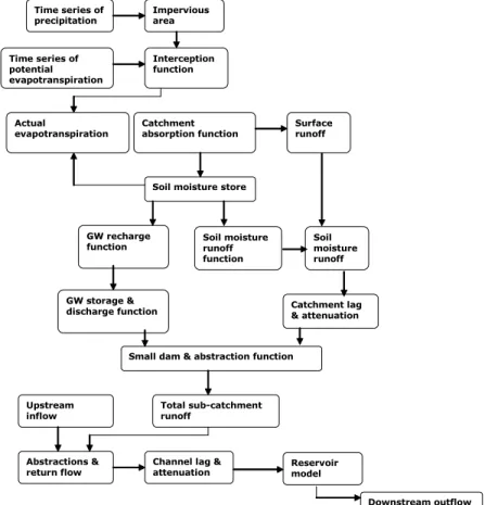
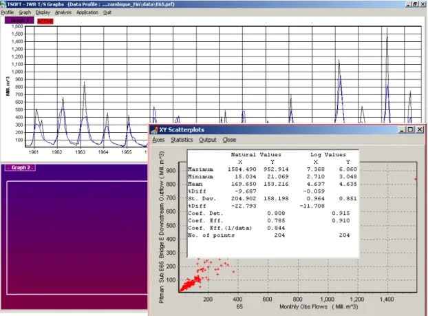
3.1 Flow diagram of the main components of the Pitman model... 34 3.2 A graphical view of the observed and the simulated in the top diagram

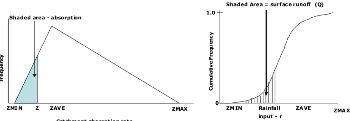
and a statistical analysis of the goodness of fit in the TSOFT analysis program of SPATSIM... 40 4.1 Illustration of a left-skewed non-symmetrical triangular frequency

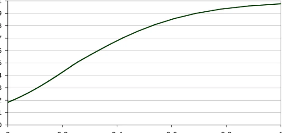
distribution of basin absorption rate, Z (left side) and the cumulative frequency curve illustrating the proportion contributing to surface

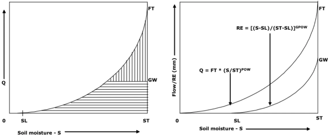
runoff generation (right side)... 48 4.2 Illustration of the relationship between ST, GW and FT and the

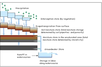
subsurface runoff generation parameters as used in PITMGW... 52 4.3 Illustration of the conceptualization of the moisture storages of the

PITMGW model ... 53 4.4 Relationship between basin evaporation (E) and soil moisture (S)

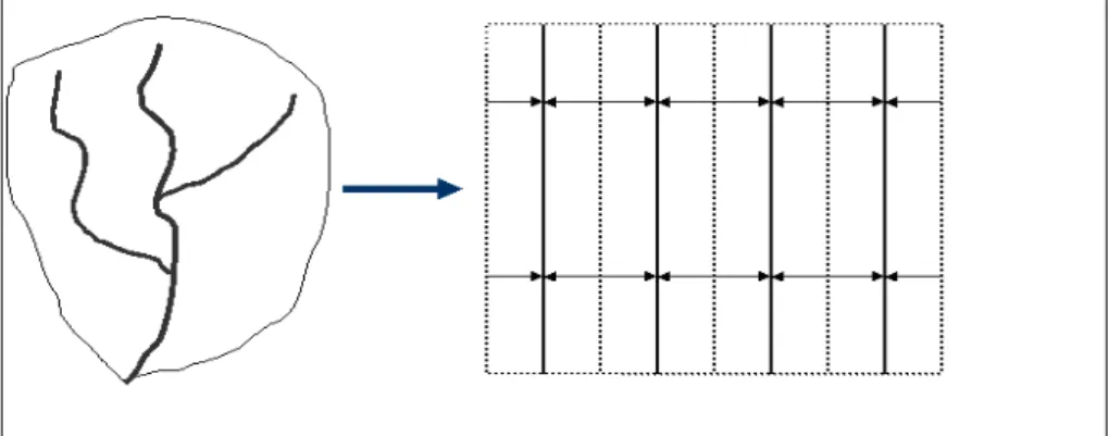
for R= 0 (A) and R = 1 (B)... 60 4.5 Conceptual representation of drainage in the basin where the channels

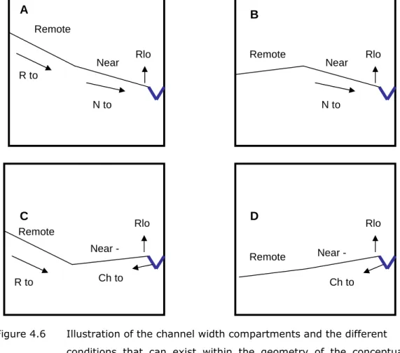
are of unit length and DDENS of 4/sqrt (Area)... 64 4.6 Illustration of the channel width compartments and the different

conditions that can exist within the geometry of the conceptual aquifer. 67 4.7 Shape of the power relationship between current month discharge

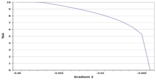
relative to a maximum value and a model variable, TLQ………….………. 71 4.8 Shape of the power relationship between current down slope gradient

and a model variable, TLG. The maximum value of TLG is defined by a model parameter….………..………. 72 5.1 Approaches to parameter estimation and model regionalization used in the

southern African region (A) and the proposed new approach (B)... 84 5.2 Illustration of the default basin property and parameter estimation

Program... 86 5.3 Conceptualization of the subsurface drainage that determines the

interflow process from the unsaturated zone... 88 5.4 Default estimation approach for the drainage vector slope... 89 5.5 Illustration of the concept of using a frequency distribution to describe

the spatial distribution of soil moisture for different mean moisture

contents... 95 5.6 Runoff-moisture content relationships for four conditions (defined by the

moisture distribution parameter, SDEV)... 96 5.7 Runoff-moisture content relationships for the same basin without

FTunsat (left side) and with FTunsat (right side)... 97 5.8 Illustration of the use of the default estimation procedures for the

surface runoff parameters (ZMIN, ZAVE and ZMAX)... 100 5.9 Illustration of the estimation of ZMIN, ZAVE and ZMAX for two

situations. The diagram on the left represents sandy soils of moderate depth with ZMIN = 30, ZAVE = 415 and ZMAX = 800. The diagram on the right represents crusted clay soils of moderate depth with

ZMIN = 0, ZAVE = 120 and ZMAX = 350... 102 6.1 The distribution of mean annual evapotranspiration (MAE) and mean

annual precipitation (MAP) over southern Africa. The MAP is a 40 year average for the period between 1950 and 1989... 104 6.2 Illustration of the detail of soils information from Zimbabwe. The map

shows part of the Mzingwane catchment with the locations of the basins for gauging stations B15, B29, B56, B77 and B78... 106 6.3 Illustration of the spatial scales and the level of detail of the soils

information available in southern Africa. The figure shows a part of the FAO maps for South Africa and a land type for a part of the

Eastern Cape... 107 6.4 Illustration of the degree of variation of the ST, FT and POW parameter

(9)

values and the number of basins with this change... 113 6.5 Results of model simulations using WR90 and the revised parameters

compared to the observed flow for the Little Boesmans river at gauging station V7H012 (A) and the Bree river at gauging station H1H003 (B). 117 6.6 Results of model simulations using the revised parameter estimation

methodology for the Macheke system at gauging station E19 in Zimbabwe (A) and for the Pungwe river system at the Pungwe Bridge (gauging station E65) in Mozambique (B)... 119 6.7 An uncertain extreme high flow value in the Pungwe basin at F14 recorded for March 1976... 121

(10)

List Of Tables

3.1 A list of the parameters of the Pitman model including those

of the reservoir water balance model... 38 5.1 Soil texture classes according to USDA (1969), based on percentage

volumes of sand, silt clay and quartz content... 87 5.2 Comparison of values of hydraulic conductitivity (in m d-1_{) by three}

estimation methods (F, G, H = 1 in column 4)... 92 5.3 Results of default estimation procedure for FTsoil (mm month-1)... 92

6.1 The distribution of the lengths of modelling periods for the basins

in the study... 110 6.2 Brief descriptions of the physical attributes of some basins

investigated in the study... 112 6.3 Basin property data, the parameters from the physically based

parameter estimation methods and results of model simulations... 114 6.4 An analysis of the results of model simulations based on the four

of the six objective functions used... 120 6.5 Analysis of the model simulations using the percentage deviation

of the simulated mean flow from the mean of the observed

flow (%M) ... 122 6.6 Comparison of estimated soil depth and porosity used to assess data

from the Atlas against the estimates used in this study... 124 6.7 Estimated parameters and the results of model simulations for 6 of the

basins using the basin property data from the Atlas (Atlas data) compared with the initial parameter estimates using the

revised procedures... 126

(11)

1

INTRODUCTION

1.1 Background

The complexity of current water resource management poses many challenges. Water managers need to solve a range of interrelated water dilemmas, such as balancing water quantity and quality, flooding, drought, maintaining biodiversity and ecological functions and services. The reliable quantification of hydrological variables such as rainfall and streamflow is a prerequisite for sustainable water resource management, planning and development within basins. Southern Africa's hydrological regime is characterized by high variability and low runoff coefficients with less than 15% conversion of mean annual precipitation (MAP) to mean annual runoff (MAR) known to be present across large parts of the region (Walmsley, 1991). With predictions of water scarcity conditions, due to rapid population growth, expanding urbanization, increased economic development and climate change, being predicted for the region (Rosegrant and Perez, 1997), water looks set to become a limiting resource in Southern Africa. The dynamics of demand and supply will have a large impact on the future socio-economic development of the region (Basson et al. 1997; Rosegrant and Perez, 1997). The other huge problem in southern Africa is the trans-boundary nature of a number of the river systems (e.g. the Zambezi, Limpopo, Orange, Okavango). This makes decision making for both the present and the future very difficult and uncertain and it is imperative to create a common platform for the quantification of this precious resource.

It is therefore prudent to be able to quantify the water resource adequately for meaningful management decisions, not only for the present but also for the future. However, data paucity as a result of shrinking measurement networks due to economic and manpower problems (Hughes, 1997; Oyebande, 2001) has had a limiting effect. Some of the major river systems in the region have been gauged for the determination of hydrological variables, but this has not been the case with most medium and small sized basins. Even so, there are several major basins in different parts of the region that are not adequately gauged and in some basins the existing gauging networks are being discontinued; this leads to uncertainty in the design of water resource systems. However, in spite of these problems water resource developments must continue to take place to satisfy the economic and social development needs of communities (Mazvimavi, 2003). To alleviate the problem of data paucity, hydrological and ecological simulation

(12)

models have been used extensively in the region and water resource planning has thus often been highly dependent on their results. The Pitman model (Pitman, 1973) is an example.

The Pitman model has grown to be a widely used hydrological assessment tool in the Southern African region and it is the author’s conviction that it could be used to a greater extent in the future. Its simplicity and user-friendly interface make it an attractive option and its data requirements are quite simple and easily met by most of the region’s hydro-meteorological agencies. The major limitation of the Pitman model is the number of model parameters that need to be optimized which often makes it harder to apply consistently in data scarce regions like southern Africa. However, with the current impetus in hydrology being the improvement of methods that enable hydrological predictions to be made in basins with limited or no historical measurement records and the reduction of the uncertainties associated with these predictions (Sivapalan, et al., 2003), the problem may be resolved. This study is borne out of the initiative of the International Association of Hydrological Sciences (IAHS) for predictions in ungauged (PUB).

The most popular of the traditional methods for prediction in ungauged basins has been the use of parameter regionalization. This involves the calibration of the model against naturalized observed flows and then developing statistical relationships between the parameters and some basin physical attributes or using some parameter mapping based on basin similarities. Two problems have always dogged regionalization in southern Africa – the limitations of flow monitoring networks mean there are generally limited reliable observed data for the calibration of the model and that there are quality issues with the data that are available. Unquantified upstream water use and abstractions mean that there are uncertainties with regards to the extent to which the observed flow data represent the natural hydrology of the basins. Given that there are other data collected by various agencies across the region (e.g. soil hydraulic properties, geology) that can be used to aid the understanding of the rainfall-runoff transfer process, this study therefore addresses the question of whether physical basin properties and the role they play in runoff generation can be used directly in the estimation of parameter values. If the answer is yes, then it may be possible to develop procedures for parameter estimation in ungauged basins that are less reliant on limited calibration results that are themselves likely to generate values with a degree of uncertainty.

(13)

There are a total of 41 parameters (only 11 are free/calibration parameters, the rest are estimated from basin properties) in the version of the model being used and the focus of this study is on the 7 calibration parameters that control the soil moisture accounting, runoff and recharge and the soil surface infiltration routines The prospect of ‘free simulations’ (using the model without calibration) would then be possible and could be used to generate flows in data scarce areas and ungauged basins. While there might be issues with the use of free simulations, they are definitely better than not having any information at all (Bergstrom, 1991). More robust parameter estimation procedures based on the physical basin characteristics may reduce the uncertainties associated with these.

1.2 Aims and Objectives

While the ultimate goal of a study of this nature would be to develop regional parameter sets for southern African basins similar to those established during the South African water resources assessment project of the 1990s (Midgley et al., 1994), the main aim of this study is to produce revised and improved calibration and application (in ungauged basins) procedures for the Pitman model in southern African basins under different climate, topography, geology, soils and vegetation conditions. This involves the estimation of parameters using conceptually physically sound principles which can be related to measurable basin characteristics and would be easier to evaluate in ungauged basins. A key goal in the development of the estimation procedures is to minimize the need for a basin-specific model calibration, and to achieve this, the model parameterization is to be structured around the use of basin physical and hydro-meteorological data.

To achieve this overall the following specific aims are envisaged for the study:

i. To develop a conceptual framework for the physical interpretation of the Pitman model parameters.

ii. To develop equations for the direct estimation of model parameters from physical basin property data.

iii. To generate sets of parameters for the Pitman model for selected basins in southern Africa.

iv. To assess the simulation results based on the use of revised estimation procedures in selected basins within southern Africa.

(14)

1.2.1 Developing a conceptual framework for the physical interpretation of the Pitman model parameters

Before physically-based estimation procedures can be developed for the Pitman model, it is essential to revisit the conceptual structure of the model and the way in which this relates to real hydrological processes. In doing this it is also necessary to consider the spatial and temporal scales at which the model is typically applied. To achieve this requires that the effect of each parameter be isolated and studied in depth to identify their physical meaning. This is what is meant by a conceptual framework for the interpretation of the parameters.

1.2.2 Developing equations for the direct estimation of model parameters from physical basin property data.

The conceptual framework will identify the specific hydrological response effects of each parameter. Using well understood principles of conceptual physical hydrology it should be possible to identify the physical basin properties that are relevant to individual parameters and develop equations that can be used to estimate the parameters. Once again, scale effects will need to be considered as will the typical availability of basin property data.

1.2.3 Generating sets of parameters for selected basins

Generating parameter sets for selected basins in the region requires the collection of appropriate basin property data. It was recognized at the start of the study that the sources, spatial resolution and accuracy of such data would vary considerably within the region, and clearly affect the results. However, this is part of the reality of applying estimation procedures in data scarce regions. Only the soil moisture accounting, recharge, runoff and soil surface infiltration parameters are being investigated and the other parameters would have to be calibrated where no regionalized parameter sets currently exist. For South Africa where regionalized parameter sets exist, those parameters estimated by the revised procedure will be used with existing parameters (not part of the new procedures) and with the same input data (rainfall and evaporation) used within the WR90 database (Midgley, et al., 1994).

(15)

1.2.4 Testing the parameters from revised estimation procedures in selected basins

The revised parameter set will be used in the model and the simulation results compared with observed flow data as well as previously established results using WR90 parameter sets in the case of South African basins. The results comparisons will be based upon a standard set of statistical criteria. One of the issues to consider is that few southern African observed flow data are completely natural, while it is often difficult to properly quantify the upstream development impacts. This issue will necessarily have to be considered in the selection of the test basins and in the interpretation of the results.

1.3 Research Questions

This study directly explores some of the principle issues associated with PUB, uncertainty analysis (though this part is not specifically covered in this study) and the practical application of hydrological models, in particular the Pitman model (Pitman, 1973), in a data scarce region such as southern Africa. The study will attempt to provide answers to the following questions:

i. How can we estimate hydrologically relevant model parameters?

ii. Can model parameters be defined in a physical manner that is consistent with physical hydrology principles?

iii. What are the optimal process conceptualizations for parameter estimations?

iv. What are the physical basin characteristics that affect model parameters? v. What relationships exist between the parameters and the physical basin

characteristics?

vi. What are the most robust ways of estimating parameters? Given the availability of data in southern Africa.

vii. What alternative sources of data can be used to aid the parameter estimation procedures?

viii. How can this knowledge be used to develop new guidelines for the calibration and application of the model?

It is accepted that models are generally quite simplified representations of reality whose parameter quantification is one of the major sources of uncertainty. This is especially so for conceptual models like the Pitman model. Therefore, in

(16)

attempting to answer these questions a number of science issues would naturally arise and these would also need attention during the whole process. The issues that arise in this study are related to the following questions:

i. What are the limits of available data sets and what new data are required? ii. Are there alternative conceptualizations (at the appropriate model spatial

and temporal scales) of the natural hydrologic processes that will facilitate better parameter estimation procedures?

iii. What are the criteria for acceptability and are these sufficient?

iv. What is the uncertainty of using these estimation methods? How does this uncertainty propagate to the ungauged basin? What would the risk be in practice?

1.4 Expected research outputs and research justification

Given the regional situation, this study has the potential to provide a practical solution for water resource managers who are often called upon to make hydrological predictions in data scarce areas for long term, highly capitalized water resource development projects. It is realistic to believe that the Pitman model will remain to be a standard hydrological tool in the southern African region for a long time to come. The scope of use of the model will also continue to rise as more uses of the model are discovered. Chief among these may be the need to model water resource impacts of climate change. Published results indicate that climate model results at the monthly time resolution have been more reliable than at shorter time scales. Thus the Pitman model could possibly be used in the forecasting of water resource scenarios in analyzing and planning for the impacts of climate change (Hughes, 2004b). Simple, more objective and robust parameter estimation procedures can only be beneficial to the southern African community of water practitioners. The non-reliance of the proposed estimation methods on limited calibration results means that improved model regionalization could be achieved. In addition, a reduction in the subjectivity associated with traditional regionalization of model parameters could create greater common understanding across the region and foster improved relationships in trans-boundary river systems.

The study is expected to produce revised, physically-based estimation procedures for the soil moisture accounting, runoff, recharge and infiltration parameters of the Pitman model for some selected basins in southern Africa.

(17)

This desktop study has been designed to cover a number of selected basins in southern Africa. 71 basins were selected for the study and were chosen to span the range of basin physical and hydro-meteorological conditions obtaining in the region. In order to reach reliable conclusions it was necessary that the data be of reasonable length of at least 25 years, covering the hydrological and climatological regimes of any chosen basin. The data relevant for this study are monthly streamflow, precipitation and evapotransipration records. The data have been accessed from published information, on-line databases and through direct contact with the relevant data collection agencies. For the streamflow data it was considered appropriate to avoid using basins where the observed data are expected to be substantially impacted by upstream developments. Notwithstanding the time factor, naturalizing the flows demands the availability of records related to storage, abstractions or return flows which are frequently difficult to obtain in the region. Therefore, only basins with as near natural flow as possible, or with minimal human impact, would be chosen.

The remainder of this document consists of chapter 2 which contains a discussion of hydrological modelling with an emphasis on southern Africa. Chapter 3 gives a brief introduction to the Pitman model (Pitman, 1973) and its application as part of SPATSIM (Spatial and Time Series Information Modelling) framework software. This is followed by a detailed description of the model and its parameters which establishes the conceptual framework on which this study is based in chapter 4. A description of the developed parameter estimation procedures follows in chapter 5. Results are presented in chapter 6 with the discussion, conclusions and recommendations finalizing the report in chapter 7.

(18)

2

RAINFALL-RUNOFF MODELLING

2.1 Introduction

A model is a mathematical or physical analogue of a natural system (Linsley, 1981). It represents an abstraction of complex reality into a form that is more easily understood. Models are therefore simplified representations of the real system which is too complex to formulate in detail and their goal within the scientific community is to help understand the operation of and make predictions the real system (Corwin, 1996). The fundamental hydrological problem is the derivation of a relationship between basin rainfall and the resultant runoff. Hydrological modelling has its roots in the work of Pierre Perrault in 1674 whose endeavors to describe the relationship between basin runoff and rainfall resulted in a simple equation: Q = P/6, where Q and P were the annual runoff and precipitation respectively (Linsley, 1981). Other early hydrologists such as Edme Mariotte (1620 – 1684) and Edmond Halley (1608 – 1680) had almost the same relationship. Many developments have followed this pioneer work to the various models of varied description and complexity that are in operation today the world over. Hydrological modelling experienced a boom in the 1970s largely as a result of advances in computing technology.

A casual search for literature (e.g. ScienceDirect on Elsevier gives about 1200 articles) on hydrological modelling reveals many hundreds of papers covering a wide variety of approaches. There are those that focus on the hydrological understanding of the modelling process where physical hydrology principles drive the modelling process. Physical concepts are studied and understood before a decision on their adequate representation in a model is taken. Some deal exclusively with the mathematics of modelling in which emphasis is on such issues as the solutions to differential equations, optimization methods, objective functions, etc. The hydrological content is often very small, the focus being on mathematics. The last approach has been to deal essentially with the ‘modelling’ issues themselves where attention has been on the improvement of model efficiency, issues of uncertainty and equifinality (Beven and Binley, 1992) and the type of equations that models can use. With such a variety of approaches, it is a daunting task in the early 21st_{century to embark on a comprehensive review of}

(19)

2.2

Model types and structure

This section attempts a description of the various model types and structures that have been used since the advent of modern day hydrological modelling. This discussion is not meant to be exhaustive but merely provide background to the current study. Models fall into many different classes. In an early treatise on hydrologic modelling, Clarke (1973) identifies two broad model classes. Models are classified on the basis of their description of the natural phenomenon into either regression or process-based models. Regression models recognize that hydrological events depend on chance and make use of historical hydro-meteorological time series data (e.g. rainfall and streamflow) and statistical principles to predict output in line with statistical patterns. On the other hand, process-based models use mathematical equations to describe hydrological phenomena in a particular basin based on the hydrological processes perceived to be in operation. The following is a small subset of process-based models; HBV (Bergstrom and Forsman, 1973), NAM (Nielsen and Hansen, 1973), Pitman (1973), TOPMODEL (Beven and Kirkby, 1979), ACRU (Schulze, 1986), IHACRES (Jakeman et al., 1990), VTI (Hughes and Sami, 1994), MIKE SHE (Refsgaard and Storm, 1995), Tank (Sugawara, 1995) and ARNO (Todini, 1996).

The process-based hydrological models can further be subdivided into either stochastic or deterministic in nature with the former assuming a randomness or uncertainty in the simulated output as a result of uncertainties in input variables (Beven, 2001). The latter relate to a simulation that allows only one outcome from given inputs on the assumption that processes can be defined in physical terms without a random component (Beven, 2001; Linsley, 1981) and are therefore chance independent (Clarke, 1973). Thus, the processes of transfer of rainfall to runoff are assumed to be governed by definite physical laws and a basin is a not a random assemblage of independent parts but an integrated physical system whose temporal and spatial variation can be adequately described (Pitman, 1973).

Deterministic models can further be classified as either empirical/metric or conceptual or physical. Empirical models are observation–oriented and characterize system response by extracting information from existing data (Kokkonen and Jakeman, 2001). This type of model is therefore essentially used to predict, but not explain, system function. Their development takes little or no cognizance of the features or processes of the hydrological system. There is no

(20)

perceived attempt to understand the rainfall-runoff hydrological processes operating within a basin. The models require records of both river flow and rainfall for calibration, use curve fitting procedures and generally cannot be applied to the ungauged situation without modification. The roots of such models can be traced back to the unit hydrograph theory by Sherman in the 1930s which is based on the assumption of a linear relationship between rainfall excess and runoff. The Rational Method is another example of this type of model (Kokkonen, 2003). To reproduce the basin-wide streamflow response to climate inputs with an empirical model, it would suffice to have a lumped loss function, to account for processes such as evaporation, interception, surface and sub-surface moisture storage and groundwater recharge, and a routing function, to represent the different components of a basin’s response (Wheater, 2005).

A physically-based process-oriented model is a simplified version of the real hydrologic system and tries to reproduce as much of the hydrological behaviour of a basin in the rainfall to runoff transfer process as possible. It is based on the generic understanding of the physics of the basin hydrological processes. Physical models recognize the entire basin as a spatially variable system and attempts to model a range of processes operating at small scales like a hill-slope to those in the entire basin. The basin is generally divided into a network of interlinked component segments for which all significant hydrological parameters are assumed to be measurable in the field. Complex mathematical relationships such as partial differential equations are normally solved numerically to describe the hydrological processes. The first of such models was developed in the 1970s in which finite difference methods were used to solve the Richards’ equation for two dimensional unsaturated flow to represent slope hydrological processes. The Systeme Hydrologique Europeen (SHE) (Abbott et al, 1986; Bathurst, 1986) model is one of the well known physical models developed along similar lines. While these models may provide mathematically sound representation of hydrological physics, usually at smaller scales, they require comprehensive data and extensive computations. The models are, however, characterized by parameters that are, in principle, measurable and have a direct physical interpretation. Theoretically, therefore, if the parameters could be determined a priori, then such models could be applied to ungauged basins and the effects of basin climate variability or land use change explicitly represented. They should be appropriate for integrated basin modelling where considerations such as land use changes and/or climate variability, movements of pollutants and sediments and groundwater recharge are important outputs, e.g. the ACRU model (Schulze,

(21)

1995) and the SWAT model (Arnold and Allen, 1996). However, this has not been achieved in practice owing to the massive extent of the data demanded by such models and the simple fact that such data are not easily available or measured. The transfer of physics-based equations developed in the laboratory at very small scales to the typical modelling scale of a basin is not an easy task (Beven, 1989). The issue here is whether it would be possible to apply theoretical equations in the field, even at relatively small scales where there is extensive natural heterogeneity. This variation in physical basin properties is an important limitation in the wider application of physical models. Physically-based models are therefore more suitable for small scale research studies where the effects of basin heterogeneity and variability of parameters is small (Bergstrom, 1991).

Conceptual models represent a compromise between the two extreme modelling approaches outlined above. Conceptual models have proved to be the most common and parsimonious model type. Conceptual models describe all the component processes of the hydrological cycle considered important in a system. The natural hydrological system is represented as a system of interconnected storages, which would be recharged and depleted by appropriate component processes of the hydrological system. In this system moisture accounting of the input of rainfall is partitioned and routed to eventually produce runoff. The level of conceptualization of such a model reflects the extent to which the model structure and its parameters are representative of basin-scale hydrological processes. This approach is thus essentially semi-physical, where an understanding of the hydrological processes and process representation are integral to the modelling philosophy, but without comprehensive detail as in the physical models. The sizes of the moisture storages, moisture routing between these storages and the output of runoff are all described via mathematical equations (Nash and Sutcliffe, 1970). Besides the coefficients of the mathematical relationships, called parameters, which vary spatially and at times temporally, the core structure of the mathematical relationships is assumed to be constant for all basins. Beven (2001) and Corwin (1996) outline the components of the classical conceptual modelling process as model perception, conceptualization, verification, sensitivity analysis, calibration and validation. The conceptual model form became popular in the late 1960s and early 1970s thanks to computing power which then made possible an integrated approach to the land component of the hydrological cycle, albeit using simplified relationships, to generate continuous flow (Wheater, 2005). The application of this type of model to a basin usually requires the quantification of the parameters that describe the model in that

(22)

particular basin and, for their extension to the ungauged basin, the development of relationships between the parameter sets and the basin physiographic characteristics. An attendant risk of conceptual modelling is that as the number of component processes increases so would the number of parameters and the uncertainties associated with their quantification. The Pitman (Pitman, 1973), the HBV (Bergstrom and Forsman, 1973), and the Sacramento (Burnash, et al., 1973) models are examples of the conceptual model type. Since their demand for input data is usually, though not always, minimal, conceptual models can be used in areas of data deficiency, making them practical and useful tools in operational hydrology. They are used mostly in hydrological forecasting (e.g. the operational flood forecasting system in the United states is based on the Sacramento model and in Sweden and Finland the HBV model is used), reservoir operation (e.g. HBV in Sweden) and in the extension of and filling in of gaps in observed records. They are also used extensively for a wide variety of water resource assessment studies (for example, Midgley et al., 1994).

Another distinct classification recognizes deterministic models as being either lumped or distributed. This classification is based on the spatial description of basin processes. A lumped model is one in which the parameters, inputs and outputs are spatially averaged for the whole basin. In a distributed model the basin is treated as a spatially variable system with all variables and parameters being allowed to vary spatially in response to differences in basin characteristics as well as rainfall and other climatic variables. There are two main groups of distribution system – one based on rectangular grids and the other on the use of natural drainage units. These drainage units vary in size from small hill-slopes or first order basins to larger basins such that the model network consists of lumped models connected by some routing system. Parameter quantification in lumped models usually requires that a historical observed flow record be available against which the model is calibrated. The parameters are averages over a basin and do not usually have any ‘true’ physical meaning. This unfortunately limits the applicability of such models beyond the areas for which they have been calibrated and their use in ungauged basins is problematic. However, a concise and unambiguous physical interpretation of the parameters should extend their applicability. In a fully physically-based distributed model attempts are made to infer parameter values from measurable physical and hydro-meteorological basin properties, thus rendering calibration unnecessary when sufficient data are available. In reality, however, some calibration is often necessary as it is impossible to characterize all the spatial and temporal variability of the

(23)

parameters at the basin scale. This is the typical model scale for most practical purposes in water resource assessments and planning and is generally larger than the design scale of distributed models. Thus, some lumping is inevitable and the parameters become spatial averages rather than direct point values from field measurements. The ‘probability distributed’ approach of Moore (1985), who suggested that ‘sub-grid’ or ‘sub-basin’ effects could be accounted for through probability distribution functions representing the (largely unknown) variations in process functioning (and therefore parameter values) within a spatial unit, could be used. The parameters of a distributed model can, at least in theory, be validated by field measurements. This should make them more reliable to use in ungauged basins. In general, however, the large data requirements and structural complexity of distributed models make them less favorable for routine use than their normally parsimonious lumped counterparts.

Hughes (2004b) considers a classification based on model complexity. Model complexity is envisaged as “the extent to which the model attempts to represent the many and diverse processes that affect the response of runoff to rainfall”. More complex models would attempt to explicitly represent all hydrologic processes (of interception, infiltration, soil water drainage, evapotranspiration, groundwater movement, etc) in a basin. This inevitably means more parameter space and more time, effort and information required in order for them to be used with any degree of success since all parameters would have to be quantified. The fully distributed process-based model types are a good example of the more complex type. Three methods of classifying models, spatial complexity, temporal complexity and model purpose, are identified. A “spatially complex” model is one in which the total basin is disaggregated into a number of sub-basins based on natural drainage units (e.g. slopes, channels, basins) or on geometric shapes (square grids, polygons, etc). The rationale of adopting this approach is that the parameters and the variations in input climatic data may be realistically represented, with limited heterogeneity, within smaller units of the total basin.

“Temporal complexity” groups models based on the time-step used. Time steps can vary from coarse intervals of a month or more, to fractions of an hour and to variable time scales (Hughes and Sami, 1994; Hughes, 1993a). With smaller time intervals, it is possible to simulate more realistically and in greater detail such rapidly changing hydrologic responses as floods. The two classes discussed above are not necessarily independent of each other and the separation in the discussion has only been for convenience. For each model structure a choice is

(24)

made about the methods appropriate for the representation of the hydrologic processes and this decision necessarily influences the time interval of modelling and the spatial distribution system to be used. Lastly, “modelling purpose” groups models according to the type of outputs generated. While some models simulate single events only, there are a number that are designed to be multi-purpose and generate a wide array of continuous information such as moisture status, groundwater levels, channel transmission losses and recharge (see Hughes and Parsons, 2005).

Even though more complex models use more input data and have a more detailed process description there is no obvious relationship between model complexity and the quality of simulation results (WMO, 1975). In fact the more complex a model is, the more likely the problem of over-parameterization and the attendant parameter interdependencies. Such structurally complex and distributed models have been useful for research and process investigation and understanding. Simple, general water balance models can work fairly well for most practical hydrological purposes even though they may not represent the physical operation of the basin in a lot of detail. Simple models therefore have a role to play in the field of water resource estimation and increasing their complexity could be counterproductive.

Notwithstanding all the various model classes, the distinction between model types is not always obvious and models firmly rooted in one approach may exhibit characteristics of a different type. In reality, therefore, almost all models are usually crossbreeds from a number of model formulations and philosophies. Many models are therefore classified as, but not limited to, lumped conceptual models, distributed physically-based or, process-oriented or semi-distributed conceptual models. The Sacramento (Burnash et al., 1973) and the Stanford Watershed model (Crawford and Linsley, 1966) are common examples of lumped conceptual models. The Pitman model (Pitman, 1993) and the HBV (Bergstrom and Forsman, 1973) are examples of semi-distributed conceptual models while SHE (Refsgaard and Storm, 1995) is a common example of a fully distributed physically-based model.

2.3

Parameter interdependence and sensitivity

Though models do vary in complexity and structure, nearly all have parameters for which values must be somehow quantified. A parameter is a quantity that

(25)

characterizes an aspect of a hydrological system in a particular basin and should remain constant in time. Parameters are distinct from variables in a hydrological system which are measurable characteristics of the system that assume different numerical values at different times (Clarke, 1973). Thus input rainfall, simulated soil moisture and both observed as well as simulated runoff are model variables. The number of parameters in a model has often been used to determine its level of parsimony as there is usually a positive correspondence between model complexity and the number of parameters. Parameters are an inherent component of all models and are basin or sub-basin specific with some having been observed to vary seasonally and still others being dependent on the spatial or temporal scales used.

Within any model, parameters exhibit elements of interdependence with each other, the extent depending on the structure and complexity of the model. Parameter interdependencies make the process of model calibration very difficult. A parameter response surface represents the value of one or more objective functions associated with results of varying two or more parameter values. Calibration is aimed at identifying the optimal location on this surface (either maximum or minimum, depending on the objective function). An objective function is a statistical function associated with an optimization problem and determines the success of a solution. It measures the match between simulated and observed time series. (see section 2.4.3). Calibration of the parameters, especially by an automatic algorithm, is thus often referred to as hill climbing in reference to the progressive attempts to get to the optimal solution. Generally optimization algorithms are categorized as either local or global where the later are designed to locate the global optimum and not be trapped at a local optimum (Madsen, 2000). Popular stochastic global search criteria include the shuffled complex evolution (SCE) algorithm (Duan et al., 1992) and genetic algorithms (GA) (Ndiritu and Daniell, 2001). The SCE has been used extensively in the calibration of conceptual rainfall-runoff models e.g. the Sacramento, NAM, Xinanjiang and the Pitman models (Gan et al., 1997) and physically-based models (see Duan et al., 1992). It has proved to be a reliable and efficient automatic optimization tool.

The interdependence characteristic of parameters has led to problems of parameter unidentifiability, over-parameterization and equifinality (Beven, 1993; 2001). A parameter is said to be unidentifiable if it cannot be estimated from a given data set. It is theoretically unidentifiable if it can never be estimated, no

(26)

matter how extensive the data set is. If the best value of a parameter depends on the values of other parameters, then it is not identifiable. On the other hand a model is said to be over-parameterized if there are too many degrees of freedom in relation to the amount of information that is contained in the observed record. Wheater et al. (2005) suggest that on the basis of information normally available in observed time series flow data, a maximum of five or six parameters would be adequate to sufficiently describe a system. This, however, seems to be an arbitrary mathematical interpretation. In practice, if models are to be used in a more physically-based manner in ungauged basin it is often necessary to have increased parameters in order to adequately describe the basin response to meteorological input. While fewer parameters may be attractive, their physical relevance is highly compromised. Calibration is then reduced to optimizing an objective function ignoring any connection between parameter values and basin properties. This problem is exacerbated in regional model calibrations where consistent and unambiguous relationships, which can be transferred to ungauged basins, are one of the objectives. Equifinality defines the existence of a number of different equally good parameter sets within a given model structure that may be acceptable in the reproduction of the observed behavior of that system (Beven and Freer, 2001). This clearly is in contradiction with the traditional concept of model calibration which is, implicitly, built on the hypothesis of the existence of a unique parameter set. While these problems are not unique to any one modelling philosophy they are more pronounced in the conceptual type of model. Normally, at the basin scale, the conceptual model approach is rather crude and almost statistical in nature, based on the assumption that the spatial variability of physical processes is not adequately known. Therefore their parameters are reduced to being just averages over a large area which often is an integral of several processes and their variability (Bergstrom, 1991). This consequently makes the physical interpretation of the parameters quite vague and difficult. Consequently the parameter response surface of conceptual models is dotted with numerous local optima making the use of local optimization search methods ineffective since the estimated optimum solution will depend on the starting point of the calibration process. The usually unknown interactions of the parameters make the parameter estimation procedure and the regionalization of parameters very difficult.

(27)

2.4

Model parameter calibration and validation

2.4.1 Model Calibration

A model structure, through its parameters, needs to be established in order to adequately simulate the hydrologic response of a specific basin to meteorological inputs. In this process the parameters are continuously adjusted until the simulated time series is a reasonable match to the observed time series data. The process of adjusting parameters to get an optimal parameter set is known as calibration. ‘Free’ parameters are those that cannot be quantified from experience, from basin property data or from other sources of information. Calibration is a necessary step in hydrological modelling, regardless of the number of parameters and the complexity of the model structure. This is because most model parameters cannot be measured, which frequently is a consequence of ambiguous physical meaning (Ao, et al, 2006). Madsen (2000) outlines the following synthesis of the objectives, in operational terms, of calibration:

i. A good water balance shown by a good agreement between the average runoff volumes.

ii. A reasonable agreement in the shapes of the simulated and observed hydrographs.

iii. A reasonable agreement in the timing, rate and volume of the peak discharges.

iv. A reasonable reproduction of the observed low flows.

What can be considered ‘reasonable’ would, however, need to be quantified for an individual basin and may depend to a certain extent on the quality of the input data and the objectives of the modelling exercise. For a successful calibration the observed record must contain sufficient signals to guide the process. While there are no hard and fast rules about the length of calibration period, it is necessary for the data to be long enough to cover the spectrum of significant events experienced in the basin (wet and dry periods, for example). The period should cover as many signals as possible and also be long enough to establish a stable parameter set. The length of record required may vary between climatic zones (Görgens, 1984). Model calibration can be achieved manually or automatically.

(28)

2.4.1.1 Manual calibration

The manual calibration technique is the traditional and used to be the more widely preferred of the two techniques. It involves the manual (or ‘expert’) adjustment of parameter values to improve the model response, based on visual inspection of the observed and simulated hydrographs and assessment using statistical measures of correspondence or objective functions. The aim is to reproduce the hydrograph peaks (amount and timing), runoff volumes, recession slopes and baseflow. A successful manual calibration calls upon the experience of the modeller and an intimate knowledge of the basic processes and interactions in the model. Thus the process can be slow, laborious and frustrating, particularly when there are many parameters to optimize and many unknown interactions between these parameters. Manual calibration can be highly subjective. However, it is the only feasible approach in areas of data scarcity (like southern Africa) where it is possible that the use of automatic calibration may lead to an optimization against inadequate signals or errors in the data. While optimization could be achieved it may be for the wrong reasons and the parameter set may not be hydrologically sensible due to calibration against errors in the data set. Manual calibration is also useful in regional calibration where it is necessary to ensure that similar basins have similar parameters, so that guidelines are developed for the use of the model in ungauged basins.

2.4.1.2 Automatic calibration

To circumvent the apparent disadvantages of the manual process, automatic techniques were developed. Automated calibration is based on optimization theory and requires the definition of a statistical measure of the differences between the simulated and observed hydrographs (i.e. objective function) and uses a mathematical algorithm to search the parameter response surface for the optimum parameter set. Also required to enable an automatic search is an observed time series against which model performance is assessed and a termination criterion to stop the iterations (Madsen, 2000). Automatic calibration has developed rapidly since the early pioneer work by Dawdy and O’Donnell (1965), Nash and Sutcliffe (1970), Ibbitt (1970) and others. The motivation for automatic techniques has been: a) the need to speed up and simplify the calibration process, b) the need to assign some objectivity and confidence to the naturally subjective manual calibrations and hence, model predictions and c) the lack of numerous expert calibrators (Hogue, et al., 2000). The Generalized

(29)

Likelihood Uncertainty Estimation (GLUE) (Beven and Binley, 1992) is an example of generic algorithms for automatic calibration of hydrologic models that has enjoyed widespread use.

The advantages forwarded in support of this method are that the computer, rather than the modeller, does the hard work of exploring the parameter space and that the procedure is relatively objective and would (at least in theory) provide, after thorough searching, a single optimum parameter set. Experience has, however, tended to disprove the later as no unique optimum parameter sets have been obtained for models (Beven, 1989; 1993; Beven and Freer, 2001). This has been attributed to the imperfect input data such as rainfall and evapotranspiration, over-parameterization or the fact that parameters, even for the physically-based process-oriented models, are only averages over heterogeneous landscapes (Wheater et al., 2005; Bergstrom, 1991). Wheater et al. (2005) further outline a number of issues that arise in automatic calibration as:

i. The existence of many local optima in the parameter space.

ii. Many known and unknown interactions among model parameters giving rise to problematic valleys, ridges and/or saddle points on the parameter response surface.

iii. Some parameters are insensitive beyond certain threshold values

iv. Scale issues e.g. where different parameters are determined at different scales making it difficult to define an optimization step size in each parameter direction when used simultaneously in a search of the response surface.

In many cases though, it is practical to use both calibration techniques to complement each other. Frequently in some conceptual models, it is wise to guide the calibration process by first roughly calibrating the model manually in order to get an acceptable, hydrologically sensible parameter set. Parameter boundaries would then be designed to constrain the subsequent automatic calibration. This ensures that the model simulations are hydrologically plausible and the simulation is for the right reasons.

(30)

2.4.2 Parameter validation

For the purposes of testing the adequacy of a calibrated parameter set in a gauged basin, it is necessary to perform a validation of the set on an independent period of the observed record. Parameter validation involves the comparison of the model output to the observed time series data with no adjustment or modification of the parameter set. Typically, validation performance statistics are worse than for the calibration period and if they are significantly lower, then questions about over-parameterization could be raised as the model might have many more degrees of freedom beyond the information contained in the observed calibration record. However, the calibration data set may also not have been representative. Klemes (1986) outlines some of the different ways of achieving a validation as;

i. Split-sample test - this is the use of two mutually exclusive subsets of the observed record.

ii. Differential split-sample test - used when the model is to simulate hydrologic response to climate and/or land-use conditions that may be significantly different from those of the available flow record, e.g. if a model was intended to simulate streamflow response to dry climate conditions it would be calibrated on a wet period and validated on the dry period.

iii. Proxy-basin test - relates to the use of one or several basins for calibration and validation in another, but homogeneous, basin. This is done, for instance, when a basin, with insufficient streamflow data, is to have its record extended. Adjustment of parameters on the basis of basin properties is allowable but not calibration.

iv. Differential proxy-basin test - is a combination of split-sample, differential split-sample and proxy basin validation. This is used for a general model aimed at accommodating all possible spatial variations.

Klemes (1986) further maintains that a model ought to be validated for the specific need and the types of application for which it is intended. Beyond these the model performance cannot be guaranteed and uncertainties are high. Besides Klemes’ methods, in multi-purpose models, designed to produce a wider range of outputs, calibration and validation may be performed on two different output variables. Such multi-criterion validation assesses the goodness of simulations of different variables when the model is calibrated with respect to another variable

(31)

(Hughes, 1993b). This should reduce the problem of equifinality and help in the assessment of parameter and model uncertainty (Wheater, 2005) and test model stability. A validation test can also be performed based on regionalization where the calibrated optimum parameter values are related to basin characteristics. This kind of validation assesses the physical soundness of both the model and the parameter estimation procedures (Seibert, 1999).

2.4.3 Assessment of model performance

Regardless of which method of calibration is used, there is always a need to assess the performance of the model in any particular basin that is being modelled. This is achieved by measuring the extent to which the simulated runoff matches the observed runoff time series. Besides a visual inspection of the two time series hydrographs, usually associated with manual calibration, more objective statistical measures are also used. A statistical method, referred to as an ‘objective function’, is normally used to objectively assess the correspondence between the two time series. The aim of the calibration process, therefore, is to optimize (either minimize or maximize depending on the type of statistical measure being used) this objective function. There is a wide variety of objective functions cited in the literature and a modelling application usually determines the ones to use. All methods aggregate the time series of the residual errors over the whole modelling period. Given that there is so much information that can be obtained from an observed flow time series, it is not possible for all the different flow components (e.g. peaks, low flows, and recessions) of the data to be sufficiently evaluated by a single performance criterion. For a complete assessment, a number of objective criteria should be used. While a more comprehensive list of objective functions can be found in Görgens (1983), a small sample of common objective functions is listed here:

(i) Coefficient of Efficiency (CE): This is the Nash and Sutcliffe (1970) model efficiency criterion. The model efficiency has become one of the most widely used measures of goodness-of-fit in hydrological modelling. CE is a dimensionless relative index of correspondence between the simulated and observed time series. Comparisons of performance can be done over different periods or basins owing to the dimensionless characteristic of CE. It is given mathematically as:

(32)

where Qobs is the observed time series, Qsim the simulated time series and Qobs is

the mean of the observed series. CE can assume any values between -∞ and 1 with the latter indicating a perfect fit between the observed and the simulated flows. When CE takes the value of zero, the simulated flow is no better estimator than the mean of the observed flows and a negative value indicates that the simulated flow is a worse estimator than the mean observed flow. CE has been observed to give relatively high values even for some visually poor simulations. It is also difficult to get high CE values in basins or periods where the variation of streamflow is low. The value of CE is sensitive to systematic errors.

(ii) Coefficient of determination, R2_{: relates to the proportion of variability}

within an observed time series data set that is explained by the simulated one. It is written mathematically as:

R2_{= ∑[(Q}

obs - Qobs)*(Qsim - Qsim)]2/[∑ (Qobs - Qobs)2 * (Qsim - Qsim)2]... 2.2

where Qsim is the mean of the simulated time series. R2 varies between 0 and 1

inclusive and _R2_{= 1 indicates that the simulated time series explains all}

variability in the observed time series, while R2_{= 0 indicates a poor}

correspondence between the two time series. While the CE is sensitive to systematic errors (general over- or under-estimation), R2 is not similarly affected and a value close to 1 does not necessarily imply a good simulation. Where both the CE and R2 are used as assessment criteria, large differences between them indicate systematic errors.

(iii) Percentage error of the total discharge volume (%V) or peak discharge (%P): these measure the percentage deviation in the total volume and peak discharge of the simulated from the observed. A perfect correspondence between the hydrographs of simulated and observed flows is shown by a value of zero with poor simulations being shown by an increasing divergence (in both directions) from zero. High values of %P and %V are an indication of systematic error. Low values of %P and %V can indicate low CE or R2 values. The percentage error of total discharge volume is written as:

(33)

where VQobs and VQsim relate to volume of observed and simulated time series

respectively. A percentage error of the mean annual runoff (MAR) can also be used and is given by:

%Mean = 100 * (MARobs – MARsim)/ MARobs ……….…… 2.4

For the %P, a threshold is defined above which all flows are regarded as peak flow events and it is expressed as;

%P = (100/Y) * ∑ (PQob