Models and Issues in Data Stream Systems
Brian Babcock Shivnath Babu Mayur Datar Rajeev Motwani Jennifer Widom
Department of Computer Science Stanford University Stanford, CA 94305
babcock,shivnath,datar,rajeev,widom @cs.stanford.edu
Abstract
In this overview paper we motivate the need for and research issues arising from a new model of data processing. In this model, data does not take the form of persistent relations, but rather arrives in multiple, continuous, rapid, time-varying data streams. In addition to reviewing past work relevant to data stream systems and current projects in the area, the paper explores topics in stream query languages, new requirements and challenges in query processing, and algorithmic issues.
1
Introduction
Recently a new class of data-intensive applications has become widely recognized: applications in which the data is modeled best not as persistent relations but rather as transient data streams. Examples of such applications include financial applications, network monitoring, security, telecommunications data manage-ment, web applications, manufacturing, sensor networks, and others. In the data stream model, individual data items may be relational tuples, e.g., network measurements, call records, web page visits, sensor read-ings, and so on. However, their continuous arrival in multiple, rapid, time-varying, possibly unpredictable and unbounded streams appears to yield some fundamentally new research problems.
In all of the applications cited above, it is not feasible to simply load the arriving data into a tradi-tional database management system (DBMS) and operate on it there. Traditradi-tional DBMS’s are not designed for rapid and continuous loading of individual data items, and they do not directly support the continuous
queries [84] that are typical of data stream applications. Furthermore, it is recognized that both approxima-tion [13] and adaptivity [8] are key ingredients in executing queries and performing other processing (e.g.,
data analysis and mining) over rapid data streams, while traditional DBMS’s focus largely on the opposite goal of precise answers computed by stable query plans.
In this paper we consider fundamental models and issues in developing a general-purpose Data Stream
Management System (DSMS). We are developing such a system at Stanford [82], and we will touch on some
of our own work in this paper. However, we also attempt to provide a general overview of the area, along with its related and current work. (Any glaring omissions are, naturally, our own fault.)
We begin in Section 2 by considering the data stream model and queries over streams. In this section we take a simple view: streams are append-only relations with transient tuples, and queries are SQL operating over these logical relations. In later sections we discuss several issues that complicate the model and query language, such as ordering, timestamping, and sliding windows. Section 2 also presents some concrete examples to ground our discussion.
In Section 3 we review recent projects geared specifically towards data stream processing, as well as a plethora of past research in areas related to data streams: active databases, continuous queries, filtering
Work supported by NSF Grant IIS-0118173. Mayur Datar was also supported by a Microsoft Graduate Fellowship. Rajeev Motwani received partial support from an Okawa Foundation Research Grant.
systems, view management, sequence databases, and others. Although much of this work clearly has ap-plications to data stream processing, we hope to show in this paper that there are many new problems to address in realizing a complete DSMS.
Section 4 delves more deeply into the area of query processing, uncovering a number of important issues, including:
Queries that require an unbounded amount of memory to evaluate precisely, and approximate query processing techniques to address this problem.
Sliding window query processing (i.e., considering “recent” portions of the streams only), both as an approximation technique and as an option in the query language since many applications prefer sliding-window queries.
Batch processing, sampling, and synopsis structures to handle situations where the flow rate of the input streams may overwhelm the query processor.
The meaning and implementation of blocking operators (e.g., aggregation and sorting) in the presence of unending streams.
Continuous queries that are registered when portions of the data streams have already “passed by,” yet the queries wish to reference stream history.
Section 5 then outlines some details of a query language and an architecture for a DSMS query processor designed specifically to address the issues above.
In Section 6 we review algorithmic results in data stream processing. Our focus is primarily on sketching techniques and building summary structures (synopses). We also touch upon sliding window computations, present some negative results, and discuss a few additional algorithmic issues.
We conclude in Section 7 with some remarks on the evolution of this new field, and a summary of directions for further work.
2
The Data Stream Model
In the data stream model, some or all of the input data that are to be operated on are not available for random access from disk or memory, but rather arrive as one or more continuous data streams. Data streams differ from the conventional stored relation model in several ways:
The data elements in the stream arrive online.
The system has no control over the order in which data elements arrive to be processed, either within a data stream or across data streams.
Data streams are potentially unbounded in size.
Once an element from a data stream has been processed it is discarded or archived — it cannot be retrieved easily unless it is explicitly stored in memory, which typically is small relative to the size of the data streams.
Operating in the data stream model does not preclude the presence of some data in conventional stored relations. Often, data stream queries may perform joins between data streams and stored relational data. For the purposes of this paper, we will assume that if stored relations are used, their contents remain static. Thus, we preclude any potential transaction-processing issues that might arise from the presence of updates to stored relations that occur concurrently with data stream processing.
2.1 Queries
Queries over continuous data streams have much in common with queries in a traditional database manage-ment system. However, there are two important distinctions peculiar to the data stream model. The first distinction is between one-time queries and continuous queries [84]. One-time queries (a class that includes traditional DBMS queries) are queries that are evaluated once over a point-in-time snapshot of the data set, with the answer returned to the user. Continuous queries, on the other hand, are evaluated continuously as data streams continue to arrive. Continuous queries are the more interesting class of data stream queries, and it is to them that we will devote most of our attention. The answer to a continuous query is produced over time, always reflecting the stream data seen so far. Continuous query answers may be stored and updated as new data arrives, or they may be produced as data streams themselves. Sometimes one or the other mode is preferred. For example, aggregation queries may involve frequent changes to answer tuples, dictating the stored approach, while join queries are monotonic and may produce rapid, unbounded answers, dictating the stream approach.
The second distinction is between predefined queries and ad hoc queries. A predefined query is one that is supplied to the data stream management system before any relevant data has arrived. Predefined queries are generally continuous queries, although scheduled one-time queries can also be predefined. Ad hoc queries, on the other hand, are issued online after the data streams have already begun. Ad hoc queries can be either one-time queries or continuous queries. Ad hoc queries complicate the design of a data stream management system, both because they are not known in advance for the purposes of query optimization, identification of common subexpressions across queries, etc., and more importantly because the correct answer to an ad hoc query may require referencing data elements that have already arrived on the data streams (and potentially have already been discarded). Ad hoc queries are discussed in more detail in Section 4.6.
2.2 Motivating Examples
Examples motivating a data stream system can be found in many application domains including finance, web applications, security, networking, and sensor monitoring.
Traderbot [85] is a web-based financial search engine that evaluates queries over real-time streaming
financial data such as stock tickers and news feeds. The Traderbot web site [85] gives some examples of one-time and continuous queries that are commonly posed by its customers.
Modern security applications often apply sophisticated rules over network packet streams. For exam-ple, iPolicy Networks [52] provides an integrated security platform providing services such as firewall support and intrusion detection over multi-gigabit network packet streams. Such a platform needs to perform complex stream processing including URL-filtering based on table lookups, and correlation across multiple network traffic flows.
Large web sites monitor web logs (clickstreams) online to enable applications such as personaliza-tion, performance monitoring, and load-balancing. Some web sites served by widely distributed web servers (e.g., Yahoo [95]) may need to coordinate many distributed clickstream analyses, e.g., to track heavily accessed web pages as part of their real-time performance monitoring.
There are several emerging applications in the area of sensor monitoring [16, 58] where a large number of sensors are distributed in the physical world and generate streams of data that need to be combined, monitored, and analyzed.
The application domain that we use for more detailed examples is network traffic management, which involves monitoring network packet header information across a set of routers to obtain information on traffic flow patterns. Based on a description of Babu and Widom [10], we delve into this example in some detail to help illustrate that continuous queries arise naturally in real applications and that conventional DBMS technology does not adequately support such queries.
Consider the network traffic management system of a large network, e.g., the backbone network of an Internet Service Provider (ISP) [30]. Such systems monitor a variety of continuous data streams that may be characterized as unpredictable and arriving at a high rate, including both packet traces and network perfor-mance measurements. Typically, current traffic-management tools either rely on a special-purpose system that performs online processing of simple hand-coded continuous queries, or they just log the traffic data and perform periodic offline query processing. Conventional DBMS’s are deemed inadequate to provide the kind of online continuous query processing that would be most beneficial in this domain. A data stream system that could provide effective online processing of continuous queries over data streams would allow network operators to install, modify, or remove appropriate monitoring queries to support efficient management of the ISP’s network resources.
Consider the following concrete setting. Network packet traces are being collected from a number of links in the network. The focus is on two specific links: a customer link, C, which connects the network of a customer to the ISP’s network, and a backbone link, B, which connects two routers within the backbone network of the ISP. Let and denote two streams of packet traces corresponding to these two links. We
assume, for simplicity, that the traces contain just the five fields of the packet header that are listed below.
src: IP address of packet sender. dest: IP address of packet destination.
id: Identification number given by sender so that destination can uniquely identify each packet. len: Length of the packet.
time: Time when packet header was recorded.
Consider first the continuous query , which computes load on the link B averaged over one-minute intervals, notifying the network operator when the load crosses a specified threshold . The functions
get-minuteandnotifyoperatorhave the natural interpretation.
: SELECT notifyoperator(sum(len))
FROM
GROUP BY getminute(time) HAVING sum(len)
While the functionality of such a query may possibly be achieved in a DBMS via the use of triggers, we are likely to prefer the use of special techniques for performance reasons. For example, consider the case where the link B has a very high throughput (e.g., if it were an optical link). In that case, we may choose to compute an approximate answer to
by employing random sampling on the stream — a task outside the
reach of standard trigger mechanisms.
The second query isolates flows in the backbone link and determines the amount of traffic generated
by each flow. A flow is defined here as a sequence of packets grouped in time, and sent from a specific source to a specific destination.
: SELECT flowid, src, dest, sum(len) AS flowlen
FROM (SELECT src, dest, len, time
FROM
ORDER BY time )
GROUP BY src, dest,getflowid(src, dest, time) AS flowid
Heregetflowidis a user-defined function which takes the source IP address, the destination IP address, and the timestamp of a packet, and returns the identifier of the flow to which the packet belongs. We assume that the data in the view (or table expression) in the FROM clause is passed to thegetflowidfunction in the order defined by the ORDER BY clause.
Observe that handling over stream is particularly challenging due to the presence of GROUP BY
and ORDER BY clauses, which lead to “blocking” operators in a query execution plan.
Consider now the task of determining the fraction of the backbone link’s traffic that can be attributed to the customer network. This query, , is an example of the kind of ad hoc continuous queries that may be
registered during periods of congestion to determine whether the customer network is the likely cause.
: (SELECT count (*)
FROM C, B
WHERE C.src = B.src and C.dest = B.dest and C.id = B.id)
(SELECT count (*) FROM )
Observe that joins streams and on their keys to obtain a count of the number of common packets.
Since joining two streams could potentially require unbounded intermediate storage (for example if there is no bound on the delay between a packet showing up on the two links), the user may prefer to compute an approximate answer. One approximation technique would be to maintain bounded-memory synopses of the two streams (see Section 6); alternatively, one could exploit aspects of the application semantics to bound the required storage (e.g., we may know that joining tuples are very likely to occur within a bounded time window).
Our final example, , is a continuous query for monitoring the source-destination pairs in the top 5
percent in terms of backbone traffic. For ease of exposition, we employ the WITH construct from SQL-99 [87].
: WITH Load AS
(SELECT src, dest, sum(len) AS traffic
FROM
GROUP BY src, dest) SELECT src, dest, traffic FROM Load AS
WHERE (SELECT count(*) FROM Load AS
WHERE .traffic .traffic)
(SELECT "! count(*) FROM Load)
3
Review of Data Stream Projects
We now provide an overview of several past and current projects related to data stream management. We will revisit some of these projects in later sections when we discuss the issues that we are facing in building a general-purpose data stream management system at Stanford.
Continuous queries were used in the Tapestry system [84] for content-based filtering over an append-only database of email and bulletin board messages. A restricted subset of SQL was used as the query language in order to provide guarantees about efficient evaluation and append-only query results. The Alert system [74] provides a mechanism for implementing event-condition-action style triggers in a conventional SQL database, by using continuous queries defined over special append-only active tables. The XFilter content-based filtering system [6] performs efficient filtering of XML documents based on user profiles expressed as continuous queries in the XPath language [94]. Xyleme [67] is a similar content-based filtering system that enables very high throughput with a restricted query language. The Tribeca stream database manager [83] provides restricted querying capability over network packet streams. The Tangram stream query processing system [68, 69] uses stream processing techniques to analyze large quantities of stored data.
The OpenCQ [57] and NiagaraCQ [24] systems support continuous queries for monitoring persistent data sets spread over a wide-area network, e.g., web sites over the Internet. OpenCQ uses a query process-ing algorithm based on incremental view maintenance, while NiagaraCQ addresses scalability in number of queries by proposing techniques for grouping continuous queries for efficient evaluation. Within the Ni-agaraCQ project, Shanmugasundaram et al. [79] discuss the problem of supporting blocking operators in query plans over data streams, and Viglas and Naughton [89] propose rate-based optimization for queries over data streams, a new optimization methodology that is based on stream-arrival and data-processing rates. The Chronicle data model [55] introduced append-only ordered sequences of tuples (chronicles), a form of data streams. They defined a restricted view definition language and algebra (chronicle algebra) that operates over chronicles together with traditional relations. The focus of the work was to ensure that views defined in chronicle algebra could be maintained incrementally without storing any of the chronicles. An algebra and a declarative query language for querying ordered relations (sequences) was proposed by Se-shadri, Livny, and Ramakrishnan [76, 77, 78]. In many applications, continuous queries need to refer to the sequencing aspect of streams, particularly in the form of sliding windows over streams. Related work in this category also includes work on temporal [80] and time-series databases [31], where the ordering of tuples implied by time can be used in querying, indexing, and query optimization.
The body of work on materialized views relates to continuous queries, since materialized views are effectively queries that need to be reevaluated or incrementally updated whenever the base data changes. Of particular importance is work on self-maintenance [15, 45, 71]—ensuring that enough data has been saved to maintain a view even when the base data is unavailable—and the related problem of data expiration [36]— determining when certain base data can be discarded without compromising the ability to maintain a view. Nevertheless, several differences exist between materialized views and continuous queries in the data stream context: continuous queries may stream rather than store their results, they may deal with append-only input data, they may provide approximate rather than exact answers, and their processing strategy may adapt as characteristics of the data streams change.
The Telegraph project [8, 47, 58, 59] shares some target applications and basic technical ideas with a DSMS. Telegraph uses an adaptive query engine (based on the Eddy concept [8]) to process queries effi-ciently in volatile and unpredictable environments (e.g., autonomous data sources over the Internet, or sensor networks). Madden and Franklin [58] focus on query execution strategies over data streams generated by sensors, and Madden et al. [59] discuss adaptive processing techniques for multiple continuous queries. The
Tukwila system [53] also supports adaptive query processing, in order to perform dynamic data integration
The Aurora project [16] is building a new data processing system targeted exclusively towards stream monitoring applications. The core of the Aurora system consists of a large network of triggers. Each trigger is a data-flow graph with each node being one among seven built-in operators (or boxes in Aurora’s terminology). For each stream monitoring application using the Aurora system, an application administrator creates and adds one or more triggers into Aurora’s trigger network. Aurora performs both compile-time optimization (e.g., reordering operators, shared state for common subexpressions) and run-time optimization of the trigger network. As part of run-time optimization, Aurora detects resource overload and performs load
shedding based on application-specific measures of quality of service.
4
Queries over Data Streams
Query processing in the data stream model of computation comes with its own unique challenges. In this section, we will outline what we consider to be the most interesting of these challenges, and describe several alternative approaches for resolving them. The issues raised in this section will frame the discussion in the rest of the paper.
4.1 Unbounded Memory Requirements
Since data streams are potentially unbounded in size, the amount of storage required to compute an exact answer to a data stream query may also grow without bound. While external memory algorithms [91] for handling data sets larger than main memory have been studied, such algorithms are not well suited to data stream applications since they do not support continuous queries and are typically too slow for real-time response. The continuous data stream model is most applicable to problems where timely query responses are important and there are large volumes of data that are being continually produced at a high rate over time. New data is constantly arriving even as the old data is being processed; the amount of computation time per data element must be low, or else the latency of the computation will be too high and the algorithm will not be able to keep pace with the data stream. For this reason, we are interested in algorithms that are able to confine themselves to main memory without accessing disk.
Arasu et al. [7] took some initial steps towards distinguishing between queries that can be answered ex-actly using a given bounded amount of memory and queries that must be approximated unless disk accesses are allowed. They consider a limited class of queries and, for that class, provide a complete characterization of the queries that require a potentially unbounded amount of memory (proportional to the size of the input data streams) to answer. Their result shows that without knowing the size of the input data streams, it is impossible to place a limit on the memory requirements for most common queries involving joins, unless the domains of the attributes involved in the query are restricted (either based on known characteristics of the data or through the imposition of query predicates). The basic intuition is that without domain restrictions an unbounded number of attribute values must be remembered, because they might turn out to join with tuples that arrive in the future. Extending these results to full generality remains an open research problem.
4.2 Approximate Query Answering
As described in the previous section, when we are limited to a bounded amount of memory it is not always possible to produce exact answers for data stream queries; however, high-quality approximate answers are often acceptable in lieu of exact answers. Approximation algorithms for problems defined over data streams has been a fruitful research area in the algorithms community in recent years, as discussed in detail in Section 6. This work has led to some general techniques for data reduction and synopsis construction, including: sketches [5, 35], random sampling [1, 2, 22], histograms [51, 70], and wavelets [17, 92]. Based on these summarization techniques, we have seen some work on approximate query answering. For example,
recent work [27, 37] develops histogram-based techniques to provide approximate answers for correlated
aggregate queries over data streams, and Gilbert et al. [40] present a general approach for building
small-space summaries over data streams to provide approximate answers for many classes of aggregate queries. However, research problems abound in the area of approximate query answering, with or without streams. Even the basic notion of approximations remains to be investigated in detail for queries involving more than simple aggregation. In the next two subsections, we will touch upon several approaches to approximation, some of which are peculiar to the data stream model of computation.
4.3 Sliding Windows
One technique for producing an approximate answer to a data stream query is to evaluate the query not over the entire past history of the data streams, but rather only over sliding windows of recent data from the streams. For example, only data from the last week could be considered in producing query answers, with data older than one week being discarded.
Imposing sliding windows on data streams is a natural method for approximation that has several attrac-tive properties. It is well-defined and easily understood: the semantics of the approximation are clear, so that users of the system can be confident that they understand what is given up in producing the approximate answer. It is deterministic, so there is no danger that unfortunate random choices will produce a bad ap-proximation. Most importantly, it emphasizes recent data, which in the majority of real-world applications is more important and relevant than old data: if one is trying in real-time to make sense of network traffic patterns, or phone call or transaction records, or scientific sensor data, then in general insights based on the recent past will be more informative and useful than insights based on stale data. In fact, for many such applications, sliding windows can be thought of not as an approximation technique reluctantly imposed due to the infeasibility of computing over all historical data, but rather as part of the desired query semantics explicitly expressed as part of the user’s query. For example, queries# and $ from Section 2.2, which
tracked traffic on the network backbone, would likely be applied not to all traffic over all time, but rather to traffic in the recent past.
There are a variety of research issues in the use of sliding windows over data streams. To begin with, as we will discuss in Section 5.1, there is the fundamental issue of how we define timestamps over the streams to facilitate the use of windows. Extending SQL or relational algebra to incorporate explicit window specifications is nontrivial and we also touch upon this topic in Section 5.1. The implementation of sliding window queries and their impact on query optimization is a largely untouched area. In the case where the sliding window is large enough so that the entire contents of the window cannot be buffered in memory, there are also theoretical challenges in designing algorithms that can give approximate answers using only the available memory. Some recent results in this vein can be found in [9, 26].
While existing work on sequence and temporal databases has addressed many of the issues involved in time-sensitive queries (a class that includes sliding window queries) in a relational database context [76, 77, 78, 80], differences in the data stream computation model pose new challenges. Research in temporal databases [80] is concerned primarily with maintaining a full history of each data value over time, while in a data stream system we are concerned primarily with processing new data elements on-the-fly. Sequence databases [76, 77, 78] attempt to produce query plans that allow for stream access, meaning that a single scan of the input data is sufficient to evaluate the plan and the amount of memory required for plan evaluation is a constant, independent of the data. This model assumes that the database system has control over which sequence to process tuples from next, e.g., when merging multiple sequences, which we cannot assume in a data stream system.
4.4 Batch Processing, Sampling, and Synopses
Another class of techniques for producing approximate answers is to give up on processing every data el-ement as it arrives, resorting to some sort of sampling or batch processing technique to speed up query execution. We describe a general framework for these techniques. Suppose that a data stream query is answered using a data structure that can be maintained incrementally. The most general description of such a data structure is that it supports two operations,update(tuple)andcomputeAnswer(). The
updateoperation is invoked to update the data structure as each new data element arrives, and the com-puteAnswermethod produces new or updated results to the query. When processing continuous queries, the best scenario is that both operations are fast relative to the arrival rate of elements in the data streams. In this case, no special techniques are necessary to keep up with the data stream and produce timely answers: as each data element arrives, it is used to update the data structure, and then new results are computed from the data structure, all in less than the average inter-arrival time of the data elements. If one or both of the data structure operations are slow, however, then producing an exact answer that is continually up to date is not possible. We consider the two possible bottlenecks and approaches for dealing with them.
Batch Processing
The first scenario is that the updateoperation is fast but the computeAnsweroperation is slow. In this case, the natural solution is to process the data in batches. Rather than producing a continually up-to-date answer, the data elements are buffered as they arrive, and the answer to the query is computed periodically as time permits. The query answer may be considered approximate in the sense that it is not timely, i.e., it represents the exact answer at a point in the recent past rather than the exact answer at the present moment. This approach of approximation through batch processing is attractive because it does not cause any uncertainty about the accuracy of the answer, sacrificing timeliness instead. It is also a good approach when data streams are bursty. An algorithm that cannot keep up with the peak data stream rate may be able to handle the average stream rate quite comfortably by buffering the streams when their rate is high and catching up during the slow periods. This is the approach used in the XJoin algorithm [88].
Sampling
In the second scenario,computeAnswermay be fast, but theupdateoperation is slow — it takes longer than the average inter-arrival time of the data elements. It is futile to attempt to make use of all the data when computing an answer, because data arrives faster than it can be processed. Instead, some tuples must be skipped altogether, so that the query is evaluated over a sample of the data stream rather than over the entire data stream. We obtain an approximate answer, but in some cases one can give confidence bounds on the degree of error introduced by the sampling process [48]. Unfortunately, for many situations (including most queries involving joins [20, 22]), sampling-based approaches cannot give reliable approximation guarantees. Designing sampling-based algorithms that can produce approximate answers that are provably close to the exact answer is an important and active area of research.
Synopsis Data Structures
Quite obiously, data structures where both theupdateand the computeAnsweroperations are fast are most desirable. For classes of data stream queries where no exact data structure with the desired properties exists, one can often design an approximate data structure that maintains a small synopsis or sketch of the data rather than an exact representation, and therefore is able to keep computation per data element to a minimum. Performing data reduction through synopsis data structures as an alternative to batch processing
or sampling is a fruitful research area with particular relevance to the data stream computation model. Synopsis data structures are discussed in more detail in Section 6.
4.5 Blocking Operators
A blocking query operator is a query operator that is unable to produce the first tuple of its output until it has seen its entire input. Sorting is an example of a blocking operator, as are aggregation operators such as SUM, COUNT, MIN, MAX, and AVG. If one thinks about evaluating continuous stream queries using a traditional tree of query operators, where data streams enter at the leaves and final query answers are produced at the root, then the incorporation of blocking operators into the query tree poses problems. Since continuous data streams may be infinite, a blocking operator that has a data stream as one of its inputs will never see its entire input, and therefore it will never be able to produce any output. Clearly, blocking operators are not very suitable to the data stream computation model, but aggregate queries are extremely common, and sorted data is easier to work with and can often be processed more efficiently than unsorted data. Doing away with blocking operators altogether would be problematic, but dealing with them effectively is one of the more challenging aspects of data stream computation.
Blocking operators that are the root of a tree of query operators are more tractable than blocking op-erators that are interior nodes in the tree, producing intermediate results that are fed to other opop-erators for further processing (for example, the “sort” phase of a sort-merge join, or an aggregate used in a subquery). When we have a blocking aggregation operator at the root of a query tree, if the operator produces a single value or a small number of values, then updates to the answer can be streamed out as they are produced. When the answer is larger, however, such as when the query answer is a relation that is to be produced in sorted order, it is more practical to maintain a data structure with the up-to-date answer, since continually retransmitting the entire answer would be cumbersome. Neither of these two approaches works well for blocking operators that produce intermediate results, however. The central problem is that the results pro-duced by blocking operators may continue to change over time until all the data has been seen, so operators that are consuming those results cannot make reliable decisions based on the results at an intermediate stage of query execution.
One approach to handling blocking operators as interior nodes in a query tree is to replace them with non-blocking analogs that perform approximately the same task. An example of this approach is the juggle operator [72], which is a non-blocking version of sort: it aims to locally reorder a data stream so that tuples that come earlier in the desired sort order are produced before tuples that come later in the sort order, although some tuples may be delivered out of order. An interesting open problem is how to extend this work to other types of blocking operators, as well as to quantify the error that is introduced by approximating blocking operators with non-blocking ones.
Tucker et al. [86] have proposed a different approach to blocking operators. They suggest augmenting data streams with assertions about what can and cannot appear in the remainder of the data stream. These assertions, which are called punctuations, are interleaved with the data elements in the streams. An example of the type of punctuation one might see in a stream with an attribute calleddaynumberis “for all future tuples, %&('*),+*-.0/*132546 .” Upon seeing this punctuation, an aggregation operator that was grouping by
daynumber could stream out its answers for alldaynumbersless than 10. Similarly, a join operator could discard all its saved state relating to previously-seen tuples in the joining stream with %&('()7+*-.0/(18946 ,
reducing its memory consumption.
An interesting open problem is to formalize the relationship between punctuation and the memory re-quirements of a query — e.g., a query that might otherwise require unbounded memory could be proved to be answerable in bounded memory if guarantees about the presence of appropriate punctuation are pro-vided. Closely related is the idea of schema-level assertions (constraints) on data streams, which also may help with blocking operators and other aspects of data stream processing. For example, we may know that
daynumbersare clustered or strictly increasing, or when joining two stream we may know that a kind of “referential integrity” exists in the arrival of join attribute values. In both cases we may use these constraints to “unblock” operators or reduce memory requirements.
4.6 Queries Referencing Past Data
In the data stream model of computation, once a data element has been streamed by, it cannot be revisited. This limitation means that ad hoc queries that are issued after some data has already been discarded may be impossible to answer accurately. One simple solution to this problem is to stipulate that ad hoc queries are only allowed to reference future data: they are evaluated as though the data streams began at the point when the query was issued, and any past stream elements are ignored (for the purposes of that query). While this solution may not appear very satisfying, it may turn out to be perfectly acceptable for many applications.
A more ambitious approach to handling ad hoc queries that reference past data is to maintain summaries of data streams (in the form of general-purpose synopses or aggregates) that can be used to give approximate answers to future ad hoc queries. Taking this approach requires making a decision in advance about the best way to use memory resources to give good approximate answers to a broad range of possible future queries. The problem is similar in some ways to problems in physical database design such as selection of indexes and materialized views [23]. However, there is an important difference: in a traditional database system, when an index or view is lacking, it is possible to go to the underlying relation, albeit at an increased cost. In the data stream model of computation, if the appropriate summary structure is not present, then no further recourse is available.
Even if ad hoc queries are declared only to pertain to future data, there are still research issues involved in how best to process them. In data stream applications, where most queries are long-lived continuous queries rather than ephemeral one-time queries, the gains that can be achieved by multi-query optimization can be significantly greater than what is possible in traditional database systems. The presence of ad hoc queries transforms the problem of finding the best query plan for a set of queries from an offline problem to an online problem. Ad hoc queries also raise the issue of adaptivity in query plans. The Eddy query execution framework [8] introduces the notion of flexible query plans that adapt to changes in data arrival rates or other data characteristics over time. Extending this idea to adapt the joint plan for a set of continuous queries as new queries are added and old ones are removed remains an open research area.
5
Proposal for a DSMS
At Stanford we have begun the design and prototype implementation of a comprehensive DSMS called
STREAM (for STanford StREam DatA Manager) [82]. As discussed in earlier sections, in a DSMS
tradi-tional one-time queries are replaced or augmented with continuous queries, and techniques such as sliding windows, synopsis structures, approximate answers, and adaptive query processing become fundamental features of the system. Other aspects of a complete DBMS also need to be reconsidered, including query languages, storage and buffer management, user and application interfaces, and transaction support. In this section we will focus primarily on the query language and query processing components of a DSMS and only touch upon other issues based on our initial experiences.
5.1 Query Language for a DSMS
Any general-purpose data management system must have a flexible and intuitive method by which the users of the system can express their queries. In the STREAM project, we have chosen to use a modified version of SQL as the query interface to the system (although we are also providing a means to submit query plans directly). SQL is a well-known language with a large user population. It is also a declarative language
that gives the system flexibility in selecting the optimal evaluation procedure to produce the desired answer. Other methods for receiving queries from users are possible; for example, the Aurora system described in [16] uses a graphical “boxes and arrows” interface for specifying data flow through the system. This interface is intuitive and gives the user more control over the exact series of steps by which the query answer is obtained than is provided by a declarative query language.
The main modification that we have made to standard SQL, in addition to allowing the FROM clause to refer to streams as well as relations, is to extend the expressiveness of the query language for sliding windows. It is possible to formulate sliding window queries in SQL by referring to timestamps explicitly, but it is often quite awkward. SQL-99 [14, 81] introduces analytical functions that partially address the shortcomings of SQL for expressing sliding window queries by allowing the specification of moving aver-ages and other aggregation operations over sliding windows. However, the SQL-99 syntax is not sufficiently expressive for data stream queries since it cannot be applied to non-aggregation operations such as joins.
The notion of sliding windows requires at least an ordering on data stream elements. In many cases, the arrival order of the elements suffices as an “implicit timestamp” attached to each data element; how-ever, sometimes it is preferable to use “explicit timestamps” provided as part of the data stream. For-mally we say (following [16]) that a data stream : consists of a set of (tuple, timestamp) pairs: :<; =,>@? BADCDFEGA >@? HADCIJEGA666JA >@?JK ADC K
EML . The timestamp attribute could be a traditional timestamp or it could be a
sequence number — all that is required is that it comes from a totally ordered domain with a distance met-ric. The ordering induced by the timestamps is used when selecting the data elements making up a sliding window.
We extend SQL by allowing an optional window specification to be provided, enclosed in brackets, after a stream (or subquery producing a stream) that is supplied in a query’s FROM clause. A window specification consists of:
1. an optional partitioning clause, which partitions the data into several groups and maintains a separate window for each group,
2. a window size, either in “physical” units (i.e., the number of data elements in the window) or in “logical” units (i.e., the range of time covered by a window, such as 30 days), and
3. an optional filtering predicate.
As in SQL-99, physical windows are specified using the ROWSkeyword (e.g., ROWS 50 PRECEDING), while logical windows are specified via theRANGEkeyword (e.g.,RANGE 15 MINUTES PRECEDING). In lieu of a formal grammar, we present several examples to illustrate our language extension.
The underlying source of data for our examples will be a stream of telephone call records, each with four attributes:customer id,type,minutes, andtimestamp. Thetimestampattribute is the ordering attribute for the records. Suppose a user wanted to compute the average call length, but considering only the ten most recent long-distance calls placed by each customer. The query can be formulated as follows:
SELECT AVG(S.minutes)
FROM Calls S [PARTITION BY S.customer id ROWS 10 PRECEDING
WHERE S.type = ’Long Distance’]
where the expression in braces defines a sliding window on the stream of calls.
Contrast the previous query to a similar one that computes the average call length considering only long-distance calls that are among the last 10 calls of all types placed by each customer:
SELECT AVG(S.minutes)
FROM Calls S [PARTITION BY S.customer id ROWS 10 PRECEDING]
WHERE S.type = ’Long Distance’
The distinction between filtering predicates applied before calculating the sliding window cutoffs and pred-icates applied after windowing motivates our inclusion of an optional WHERE clause within the window specification.
Here is a slightly more complicated example returning the average length of the last 1000 telephone calls placed by “Gold” customers:
SELECT AVG(V.minutes) FROM (SELECT S.minutes
FROM Calls S, Customers T
WHERE S.customer id = T.customer id AND T.tier = ’Gold’)
V [ROWS 1000 PRECEDING]
Notice that in this example, the stream of calls must be joined to the Customers relation before applying the sliding window.
5.2 Timestamps in Streams
In the previous section, sliding windows are defined with respect to a timestamp or sequence number at-tribute representing a tuple’s arrival time. This approach is unambiguous for tuples that come from a single stream, but it is less clear what is meant when attempting to apply sliding windows to composite tuples that are derived from tuples from multiple underlying streams (e.g., windows on the output of a join operator). What should the timestamp of a tuple in the join result be when the timestamps of the tuples that were joined to form the result tuple are different? Timestamp issues also arise when a set of distributed streams make up a single logical stream, as in the web monitoring application described in Section 2.2, or in truly distributed streams such as sensor networks when comparing timestamps across stream elements may be relevant.
In the previous section we introduced implicit timestamps, in which the system adds a special field to each incoming tuple, and explicit timestamps, in which a data attribute is designated as the timestamp. Explicit timestamps are used when each tuple corresponds to a real-world event at a particular time that is of importance to the meaning of the tuple. Implicit timestamps are used when the data source does not already include timestamp information, or when the exact moment in time associated with a tuple is not important, but general considerations such as “recent” or “old” may be important. The distinction between implicit and explicit timestamps is similar to that between transaction and valid time in the temporal database literature [80].
Explicit timestamps have the drawback that tuples may not arrive in the same order as their timestamps — tuples with later timestamps may come before tuples with earlier timestamps. This lack of guaranteed ordering makes it difficult to perform sliding window computations that are defined in relation to explicit timestamps, or any other processing based on order. However, as long as an input stream is “almost-sorted” by timestamp, except for local perturbations, then out-of-order tuples can easily be corrected with little buffering. It seems reasonable to assume that even when explicit timestamps are used, tuples will be deliv-ered in roughly increasing timestamp order.
Let us now look at how to assign appropriate timestamps to tuples output by binary operators, using join as an example. There are several possible approaches that could be taken; we discuss two. The first approach, which fits better with implicit timestamps, is to provide no guarantees about the output order of
tuples from a join operator, but to simply assume that tuples that arrive earlier are likely to pass through the join earlier; exact ordering may depend on implementation and scheduling vagaries. Each tuple that is produced by a join operator is assigned an implicit timestamp that is set to the time that it was produced by the join operator. This “best-effort” approach has the advantage that it maximizes implementation flexibility; it has the disadvantage that it makes it impossible to impose precisely-defined, deterministic sliding-window semantics on the results of subqueries.
The second approach, which fits with either explicit or implicit timestamps, is to have the user specify as part of the query what timestamp is to be assigned to tuples resulting from the join of multiple streams. One simple policy is that the order in which the streams are listed in the FROM clause of the query represents a prioritization of the streams. The timestamp for a tuple output by a join should be the timestamp of the join-ing tuple from the input stream listed first in the FROM clause. This approach can result in multiple tuples with the same timestamp; for the purpose of ordering the results, ties can be broken using the timestamp of the other input stream. For example, if the query is
SELECT *
FROM S1 [ROWS 1000 PRECEDING], S2 [ROWS 100 PRECEDING] WHERE S1.A = S2.B
then the output tuples would first be sorted by the timestamp of S1, and then ties would be broken according to the timestamp of S2.
The second, stricter approach to assigning timestamps to the results of binary operators can have a drawback from an implementation point of view. If it is desirable for the output from a join to be sorted by timestamp, the join operator will need to buffer output tuples until it can be certain that future input tuples will not disrupt the ordering of output tuples. For example, if S1’s timestamp has priority over S2’s and a recent S1 tuple joins with an S2 tuple, it is possible that a future S2 tuple will join with an older S1 tuple that still falls within the current window. In that case, the join tuple that was produced second belongs before the join tuple that was produced first. In a query tree consisting of multiple joins, the extra latency introduced for this reason could propagate up the tree in an additive fashion. If the inputs to the join operator did not have sliding windows at all, then the join operator could never confidently produce outputs in sorted order.
As mentioned earlier, sliding windows have two distinct purposes: sometimes they are an important part of the query semantics, and other times they are an approximation scheme to improve query efficiency and reduce data volumes to a manageable size. When the sliding window serves mostly to increase query processing efficiency, then the best-effort approach, which allows wide latitude over the ordering of tuples, is usually acceptable. On the other hand, when the ordering of tuples plays a significant role in the meaning of the query, such as for query-defined sliding windows, then the stricter approach may be preferred, even at the cost of less efficient implementation. A general-purpose data stream processing system should support both types of sliding windows, and the query language should allow users to specify one or the other.
In our system, we add an extra keyword, RECENT, that replaces PRECEDING when a “best-effort” ordering may be used. For example, the clause ROWS 10 PRECEDING specifies a window consisting of the previous 10 tuples, strictly sorted by timestamp order. By comparison, ROWS 10 RECENTalso specifies a sliding window consisting of 10 records, but the DSMS is allowed to use its own ordering to produce the sliding window, rather than being constrained to follow the timestamp ordering. TheRECENT
keyword is only used with “physical” window sizes specified as a number of records; “logical” windows such asRANGE 3 DAYS PRECEDINGmust use thePRECEDINGkeyword.
N(O N P NRQ SDT O P UWVYX Q UIVZX O UWVYX P
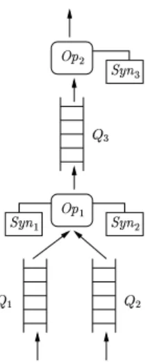
Figure 1: A portion of a query plan in our DSMS.
5.3 Query Processing Architecture of a DSMS
In this section, we describe the query processing architecture of our DSMS. So far we have focused on con-tinuous queries only. When a query is registered, a query execution plan is produced that begins executing and continues indefinitely. We have not yet addressed ad hoc queries registered after relevant streams have begun (Section 4.6).
Query execution plans in our system consist of operators connected by queues. Operators can maintain intermediate state in synopsis data structures. A portion of an example query plan is shown in Figure 1, with one binary operator ([]\*^ ) and one unary operator ([]\H_ ). The two operators are connected by a queue` ,
and operator []\7^ has two input queues,
$ and . Also shown in Figure 1 are two synopsis structures
used by operator []\*^ , a#bHc0^ and a#bHc_ , one per input. For example, []\*^ could be a sliding window join operator, which maintains a sliding window synopsis for each join input (Section 4.3). The system memory
is partitioned dynamically among the synopses and queues in query plans, along with the buffers used for handling streams coming over the network and a cache for disk-resident data. Note that both Aurora [16] and Eddies [8] use a single globally-shared queue for inter-operator data flow instead of separate queues between operators as in Figure 1.
Operators in our system are scheduled for execution by a central scheduler. During execution, an op-erator reads data from its input queues, updates the synopsis structures that it maintains, and writes results to its output queues. (Our operators thus adhere to theupdateandcomputeAnswermodel discussed in Section 4.4.) The period of execution of an operator is determined dynamically by the scheduler and the operator returns control back to the scheduler once its period expires. We are experimenting with different policies for scheduling operators and for determining the period of execution. The period of execution may be based on time, or it may be based on other quantities, such as the number of tuples consumed or pro-duced. Both Aurora and Eddies have chosen to perform fine-grained scheduling where, in each step, the scheduler chooses a tuple from the global queue and passes it to an operator for processing, an approach that our scheduler could choose if appropriate.
We expect continuous queries and the data streams on which they operate to be long-running. During the lifetime of a continuous query parameters such as stream data characteristics, stream flow rates, and the number of concurrently running queries may vary considerably. To handle these fluctuations, all of our operators are adaptive. So far we have focused primarily on adaptivity to available memory, although other factors could be considered, including using disk to increase temporary storage at the expense of latency.
Our approach to memory adaptivity is basically one of trading accuracy for memory. Specifically, each operator maximizes the accuracy of its output based on the size of its available memory, and handles dynamic changes in the size of its available memory gracefully, since at run-time memory may be taken away from one operator and given to another. As a simple example, a sliding window join operator as discussed above may be used as an approximation to a join over the entire history of input streams. If so, the larger the windows (stored in available memory), the better the approximation. Other examples include duplicate elimination using limited-size hash tables, and sampling using reservoirs [90]. The Aurora system [16] also proposes adaptivity and approximations, and uses load-shedding techniques based on application-specified measures of quality of service for graceful degradation in the face of system overload.
Our fundamental approach of trading accuracy for memory brings up some interesting problems:
We first need to understand how different query operators can produce approximate answers under limited memory, and how approximate results behave when operators are composed in query plans.
Given a query plan as a tree of operators and a certain amount of memory, how can the DSMS allocate memory to the operators to maximize the accuracy of the answer to the query (i.e., minimize approximation)?
Under changing conditions, how can the DSMS reallocate memory among operators?
Suppose we are given a query rather than a query plan. How does the query optimizer efficiently find the plan that, with the best memory allocation, minimizes approximation? Should plans be modified when conditions change?
Even further, since synopses could be shared among query plans [75], how do we optimally consider a set of queries, which may be weighted by importance?
In addition to memory management, we are faced the problem of scheduling multiple query plans in a DSMS. The scheduler needs to provide rate synchronization within operators (such as stream joins) and also across pipelined operators in query plans [8, 89]. Time-varying arrival rates of data streams and time-varying output rates of operators add to the complexity of scheduling. Scheduling decisions also need to take into account memory allocation across operators, including management of buffers for incoming streams, availability of synopses on disk as opposed to in memory, and the performance requirements of individual queries.
Aside from the query processing architecture, user and application interfaces need to be reinvestigated in a DSMS given the dynamic environment in which it operates. Systems such as Aurora [16] and Han-cock [25] completely eliminate declarative querying and provide only procedural mechanisms for querying. In contrast, we will provide a declarative language for continuous queries, similar to SQL but extended with operators such as those discussed in Section 5.1, as well as a mechanism for directly submitting plans in the query algebra that underlies our language.
We are developing a comprehensive DSMS interface that allows users and administrators to visually monitor the execution of continuous queries, including memory usage and approximation behavior. We will also provide a way for administrators to adjust system parameters as queries are running, including memory allocation and scheduling policies.
6
Algorithmic Issues
The algorithms community has been fairly active of late in the area of data streams, typically motivated by problems in databases and networking. The model of computation underlying the algorithmic work is
similar to that in Section 2 and can be formally stated as follows: A data stream algorithm takes as input a
sequence of data itemsdefA666gADdihjA666 called the data stream, where the sequence is scanned only once in the increasing order of the indexes. The algorithm is required to maintain the value of a functionk on the prefix of the stream seen so far.
The main complexity measure is the space used by the algorithm, although the time required to process each stream element is also relevant. In some cases, the algorithm maintains a data structure which can be used to compute the value of the function k on demand, and then the time required to process each such
query also becomes of interest. Henzinger et al. [49] defined a similar model but also allowed the algorithm to make multiple passes over the stream data, making the number of passes itself a complexity measure. We will restrict our attention to algorithms which are allowed only one pass.
We will measure space and time in terms of the parameter l which denotes the number of stream
elements seen so far. The primary performance goal is to ensure that the space required by a stream algorithm is “small.” Ideally, one would want the memory bound to be independent of l (which is unbounded).
However, for most interesting problems it is easy to prove a space lower bound that precludes this possibility, thereby forcing us to settle for bounds that are merely sublinear inl . A problem is considered to be
“well-solved” if one can devise an algorithm which requires at most m
>onipRqYrs>utwv x
lyEDE space andm
>onipRqYrs>utwv x lyEDE
processing time per data element or query1. We will see that in some cases it is impossible to achieve such an algorithm, even if one is willing to settle for approximations.
The rest of this section summarizes the state of the art for data stream algorithms, at least as relevant to databases. We will focus primarily on the problems of creating summary structures (synopses) for a data stream, such as histograms, wavelet representation, clustering, and decision trees; in addition, we will also touch upon known lower bounds for space and time requirements of data stream algorithms. Most of these summary structures have been considered for traditional databases [13]. The challenge is to adapt some of these techniques to the data stream model.
6.1 Random Samples
Random samples can be used as a summary structure in many scenarios where a small sample is expected to capture the essential characteristics of the data set [65]. It is perhaps the easiest form of summarization in a DSMS and other synopses can be built from a sample itself. In fact, the join synopsis in the AQUA system [2] is nothing but a uniform sample of the base relation. Recently stratified sampling has been proposed as an alternative to uniform sampling to reduce error due to the variance in data and also to reduce error for group-by queries [1, 19]. To actually compute a random sample over a data stream is relatively easy. The reservoir sampling algorithm of Vitter [90] makes one pass over the data set and is well suited for the data stream model. There is also an extension by Chaudhuri, Motwani and Narasayya [22] to the case of weighted sampling.
6.2 Sketching Techniques
In their seminal paper, Alon, Matias and Szegedy [5] introduced the notion of randomized sketching which has been widely used ever since. Sketching involves building a summary of a data stream using a small amount of memory, using which it is possible to estimate the answer to certain queries (typically, “distance” queries) over the data set.
Letz{;
>
d|BA666JADd"h$E be a sequence of elements where eachdJ} belongs to the domain~;
=
4HA666JA#L .
Let the multiplicity}]; =G
dj;CDL7 denote the number of occurrences of valueC in the sequencez . For
2{ , the
th frequency moment0 ofz is defined ass; }] } ; further, we define ;R } }. 1
The frequency moments capture the statistics of the distribution of values in z — for instance, I is the
number of distinct values in the sequence, is the length of the sequence, is the self-join size (also
called Gini’s index of homogeneity), and
is the most frequent item’s multiplicity. It is not very difficult
to see that an exact computation of these moments requires linear space and so we focus our attention on approximations.
The problem of efficiently estimating the number of distinct values ( ) has received particular attention
in the database literature, particularly in the context of using single pass or random sampling algorithms [18, 46]. A sketching technique to compute, was presented earlier by Flajolet and Martin [35]; however, this
had the drawback of requiring explicit families of hash functions with very strong independence properties. This requirement was relaxed by Alon, Matias, and Szegedy [5] who presented a sketching technique to estimate within a constant factor
2. Their technique uses linear hash functions and requires only
m
>utwv x E
memory. The key contribution of Alon et al. [5] was a sketching technique to estimate G that uses only
m
>utv x
twv x
l E space and provides arbitrarily small approximation factors. This technique has found many
applications in the database literature, including join size estimation [4], estimatingB norm of vectors [33],
and processing complex aggregate queries over multiple streams [27, 37]. It remains an open problem to come up with techniques to maintain correlated aggregates [37] that have provable guarantees.
The key idea behind the 0 -sketching technique can be described as follows: Every element C in the domain ~ is hashed uniformly at random onto a value ¡}$¢
=*£
4HAG4RL . Define the random variable ¤¥;
}
¦}Y¡J} and return ¤
as the estimator of . Observe that the estimator can be computed in a single
pass over the data provided we can efficiently compute the ¡} values. If the hash functions have four-way
independence3, it is easy to prove that the quantity¤
has expectation equal toe and variance less than
§
. Using standard tricks, we can combine several independent estimators to accurately and with high
probability obtain an estimate of . At an intuitive level, we can view this technique as a tug-of-war where
elements are randomly assigned to one of the two sides of the rope based on the value C; the square of the
displacement of the rope captures the skew in the data.
Observe that computing the self-join size of a relation is exactly the same as computing¨ for the values
of the join attribute in the relation. Alon et al. [4] extended this technique to estimating the join size between two distinct relations © and , as follows. Letª and« be random variables corresponding to© and ,
respectively, similar to the random variable¤ above; the mapping from domain valuesC to¡} is the same
for both relations. Then, it can be proved that the estimator ª« has expected value equal to ©¬®¯
and variance less than §
©®¬°©±w²¬°¯. In order to get small relative error, we can usem
>³´"µe´]³¶³·¸µ#·¹³ ³´iµ#·º³»
E
independent estimators. Observe that for estimating joins between two relations, the number of estimators depends on the data distribution. In a recent paper, Dobra et al. [27] extended this technique to estimate the size of multi-way joins and for answering complex aggregates queries over them. They also provide techniques to optimally partition the data domain and use estimators on each partition independently, so as to minimize the total memory requirement.
The frequency moment can also be viewed as the s norm of a vector whose value along the Cth
dimension is the multiplicity ¼}. Thus, the above technique can be used to compute the, norm under a
update model for vectors, where each data element
>Y½
ADC¾E increments (or decrements) some`} by a quantity
½
. On seeing such an update, we update the corresponding sketch by adding
½
¡¶} to the sum. The sketching
idea can also be extended to compute the norm of a vector, as follows. Let us assume that each dimension
of the underlying vector is an integer, bounded by¿ . Consider the unary representation of the vector. It
has ¿ bit positions (elements), where is the dimension of the underlying vector. A 4 in the unary
2
As discussed in Section 6.7, recently Bar-Yossef et al. [12] and Gibbons and Tirthapura [38] have devised algorithms which, under certain conditions, provide arbitrarily small approximation factors without recourse to perfect hash functions.
3Hash functions with four-way independence can be obtained using standard techniques involving the use of parity check matrices of BCH codes [65].
representation denotes that the element corresponding to the bit position is present once; otherwise, it is not present. Thens captures theÀ norm of the vector. The catch is that, given an elementÁY} along dimension C , it is required that we can efficiently compute the range sumÃÂIÄ@Å
F"
¡B}YÆ of the hash values corresponding
to the pertinent bit positions that are set to 4 . Feigenbaum et al. [33] showed how to construct such a family
of range-summableDZ4 -valued hash functions with limited (four-way) independence. Indyk [50] provided
a uniform framework to compute the È norm (for
n
¢
>
A §gÉ
) using the so-called
n
-stable distributions, improving upon the previous paper [33] for estimating the7 norm, in that it allowed for arbitrary addition
and deletion updates in every dimension. The ability to efficiently compute andº norm of the difference
of two vectors is central to some synopsis structures designed for data streams.
6.3 Histograms
Histograms are commonly-used summary structures to succinctly capture the distribution of values in a data set (i.e., a column, or possibly even a collection of columns, in a table). They have been employed for a multitude of tasks such as query size estimation, approximate query answering, and data mining. We consider the summarization of data streams using histograms. There are several different types of histograms that have been proposed in the literature. Some popular definitions are:
V-Optimal Histogram: These approximate the distribution of a set of values
½ BA666BA ½HK by a piecewise-constant functionÊ ½i>
C¨E , so as to minimize the sum of squared error
} >Y½ } £ Ê ½"> C¨EDE .
Equi-Width Histograms: These partition the domain into buckets such that the number of
½
} values
falling into each bucket is uniform across all buckets. In other words, they maintain quantiles for the underlying data distribution as the bucket boundaries.
End-Biased Histograms: These will maintain exact counts of items that occur with frequency above
a threshold, and approximate the other counts by an uniform distribution. Maintaining the count of such frequent items is related to Iceberg queries [32].
We give an overview of recent work on computing such histograms over data streams.
V-Optimal Histograms over Data Streams
Jagadish et al. [54] showed how to compute optimal V-Optimal Histograms for a given data set using dy-namic programming. The algorithm usesm
>
lyE space and requiresm
>
l
ËE time, wherel is the size of the
data set and is the number of buckets. This is prohibitive for data streams. Guha, Koudas and Shim [43]
adapted this algorithm to sorted data streams. Their algorithm constructs an arbitrarily-close V-Optimal Histogram (i.e., with error arbitrarily close to that of the optimal histogram), usingm
>
twv x
lyE space and
m
>
twv x
l E time per data element.
In a recent paper, Gilbert et al. [39], removed the restriction that the data stream be sorted, providing algorithms based on the sketching technique described earlier for computingF norms. The idea is to view
each data element as an update to an underlying vector of lengthl that we are trying to approximate using
the best -bucket histogram. The time to process a data element, the time to reconstruct the histogram, and
the size of the sketch are each bounded by
npHqZrs> ÌA
twv x
lÍAB4JHÎGE , whereÎ is the relative error we are willing
to tolerate. Their algorithm proceeds by first constructing a robust approximation to the underlying “signal.” A robust approximation is built by repeatedly adding a dyadic interval of constant value4which best reduces the approximation error. In order to find such a dyadic interval it is necessary to efficiently compute the