ETFs, Arbitrage, and Contagion

(1)

ETFs, Arbitrage, and Contagion

Itzhak Ben-David

Fisher College of Business, The Ohio State University

Francesco Franzoni

Swiss Finance Institute and the University of Lugano

Rabih Moussawi

Wharton Research Data Services, The Wharton School, University of Pennsylvania

November 2011

VERY PRELIMINARY,

PLEASE DO NOT QUOTE WITHOUT AUTHORS’ PERMISSION Abstract

Recent literature suggests that trading by institutional investors may affect the first and second moments of returns. Elaborating on this intuition, we conjecture that arbitrageurs can propagate liquidity shocks between related markets. The paper provides evidence in this direction by studying Exchange Traded Funds (ETFs), an asset class that has gained paramount importance in recent years. We report that arbitrage activity occurs between ETFs and the underlying assets. Then, we show that ETFs increase the volatility of the underlying assets, and that the prices of the underlying assets are affected by shocks to ETFs. Finally, we present findings consistent with the idea that ETFs served as a conduit for shock propagation between the futures market and the equity market during the Flash Crash on May 6, 2010. Overall, our results suggest that arbitrage activity may induce contagion.

____________________

(2)

2

1 Introduction

The claim that demand shocks can cause significant deviations from fundamental prices is gaining increasing popularity in the finance literature (see Gromb and Vayanos 2010 for a survey). Founded on the concept of the limits of arbitrage, a number of recent studies argue that institutional trading can significantly affect the first and second moments of asset returns. On the theory side, asset pricing models have been developed that explicitly incorporate the impact of institutions on asset prices (e.g., Basak and Pavlova 2011, Vayanos and Wooley 2011). Empirically, there is plenty of evidence on the effect of institutional investors on expected returns (Shleifer 2006, Barberis, Shleifer, and Wurgler 2005, Coval and Stafford 2007, and Wurgler 2010 for a survey) and correlations (Greenwood and Thesmar 2011, Anton and Polk 2011, Lou 2011, Cella, Ellul, and Giannetti 2011, and Chang and Hong 2011). While these studies show that institutional trading may affect asset prices, to the best of our knowledge there is no evidence on the role of arbitrageurs’ trades in the transmission of non-fundamental shocks.

Elaborating on the above literature, this paper conjectures that arbitrage activity between two related assets can transmit liquidity shocks from one asset to another. For example, if the price of one asset drops because of a decrease in demand, arbitrageurs will buy this asset and sell another similar asset that is priced correctly. The selling, however, can lead to downward price pressure on the latter asset, hence, creating a deviation from efficient pricing. In other words, the initial liquidity shock is propagated to the price of the second asset, which falls without a fundamental reason. So, one can expect that the introduction of arbitrage relations among assets, as a result of financial innovation, opens the door to faster propagation of liquidity shocks across financial markets. Ultimately, this channel can cause an increase in non-fundamental volatility for the assets that are part of arbitrage relations. This seems like an unintended consequence of arbitrage.

The paper searches for evidence on this channel of contagion by focusing on Exchange Traded Funds (ETFs). The price of ETFs is tied by arbitrage to the value of the basket of securities in the funds’ portfolio. The fact that new shares of ETFs can be created and redeemed almost continuously assures that, on average, the ETF price cannot diverge consistently and

(3)

3

substantially from its net asset value (NAV).1 Because ETFs are so popular among retail and institutional investors for speculative and hedging purposes, they are exposed to non-fundamental demand shocks. The shocks can be transmitted from the ETF to the underlying assets via the arbitrage activity that is taking place between the two. The alternative hypothesis to our conjecture is that the prices of the underlying securities are securely tied to their fundamental value because they are traded in a very efficient market. In this case, the arbitrage activity following from a non-fundamental shock to the ETF price would only move the ETF price back to the NAV.

This paper presents the first evidence that ETFs propagate shocks to the underlying assets as a result of arbitrage activity. Our main identification strategy is simple. We show that ETF mispricing is positively and significantly associated with subsequent movements in the underlying securities’ prices, after controlling for the price discovery channel. Prices move in the direction predicted by the re-establishment of the arbitrage relation. Because the effect of non-fundamental shocks to the ETF price is to generate deviations from the NAV, showing that the NAV moves to close the mispricing amounts to proving that a non-fundamental shocks to the ETF can be propagated to the underlying assets.

In the first part of the paper, we show that ETF mispricing, i.e., the difference between the ETF price and its NAV, can be non-negligible and increases with measures of limits of arbitrage. In the time series, we show that mispricing is stronger following periods of high volatility and poor stock market returns, which is consistent with the results of Nagel (2011) on the positive link between market volatility and the profitability of liquidity provision. Also, ETF mispricing is greater following periods of poor stock market returns and poor returns for the financial sector. In line with Hameed, Kang, and Viswanthan (2011), these results suggest that mispricing is larger following times in which arbitrageurs are more constrained. In the cross-section, we find that mispricing is larger for poorly performing ETFs and for ETFs with high bid-ask spread. We also document evidence for arbitrage activity as a response to mispricing: short interest in ETFs is associated with ETF prices being higher than the NAV.

1_{The ETF industry has grown at the rate of about 40% per year in the last ten years. In November 2010, assets under}

management by ETFs globally were $1.4 trillion. ETF trading, along with other Exchange Traded Products, represented about 40% of all trading volume in U.S. markets in August 2010. Source: Blackrock. Also see:

(4)

4

In the second part of the paper, we explore the idea that shocks to the prices of ETFs are transmitted to the prices of the underlying assets via arbitrage activity. First, we show that a premium of the ETF price relative to the NAV on a given day significantly predicts an increase in the NAV value on the next day. This may be the result of arbitrage, which is the channel that we want to identify. It can also result from price discovery taking place first in the ETF market, with the prices of the underlying securities following with some delay. To control for the price discovery channel, we include the return on the ETF among the right-hand side variables.

This identification strategy suggests that non-fundamental variation in the ETF price is transmitted to the price of the underlying securities. Also, we find that prices of the underlying stocks increase following a creation of new ETF units. This is likely the result of arbitrage activity, as investors convert baskets of stocks into ETFs units when ETF prices are above the NAV. To separate the effect of arbitrage from other potential explanations, we instrument the daily change in ETF shares with the mispricing in the previous day.

Second, we show a rise in the average volatility of individual stocks after ETFs increase their ownership in those stocks, while controlling for changes in ownership of other institutions. We estimate that median holding of ETFs in late 2010 caused daily stock volatility to increase by 13 basis points, a 3.4% increase. For the 90th percentile ETF ownership, the increase in daily volatility due to ETF ownership was 24 basis points, a 6.3% increase. The effect is more pronounced in small stocks, where arbitrage trading activity is expected to have greater price impact due to reduced liquidity. We take this as further evidence that ETFs operate as a conduit of shocks to the underlying securities. Volatility of the underlying assets increases because of ETF ownership as these assets inherit, via arbitrage, the non-fundamental shocks to the ETF price.

In the last part of the paper, we provide novel evidence suggesting that ETFs operated as a vehicle of contagion between the futures market and the equity market during the Flash Crash on May 6, 2010. On that day, the S&P 500 declined dramatically in value as a result of a negative demand shock originated in the S&P 500 E-mini futures market (see the CFTC and SEC 2010 preliminary and final reports). The anecdotal evidence reports cross-market arbitrage between the futures and the ETFs tracking the index. In practice, after the decline of the futures prices, cross-market arbitrageurs sold index-tracking ETFs and bought futures, driving down

(5)

5

ETF prices. We conjecture and find consistent evidence that arbitrage between the ETFs and the underlying stocks contributed to propagate the initial shock to the spot market for stocks. During the downward move in the market, the ETF discount is a significant predictor of the negative return on the S&P 500 in the following second, controlling for returns of the futures contract. As additional evidence that arbitrage-induced trading is pushing equity prices in the direction of the ETF, we report that the order imbalance on the S&P 500 stocks follows the direction of the lagged ETF mispricing.

The bottom line of the paper is that ETFs transmit shocks to the underlying assets through the process of arbitrage. These findings imply that ETFs increase the risk of contagion across asset classes, and especially so for less liquid securities. More broadly, our results potentially extend to all situations in which assets are linked by arbitrage relations. For this reason, the paper raises the topical question on the extent to which the development of derivative markets has caused an increase in volatility.

The paper proceeds as follows. Section 2 describes the data used in the study. Section 3 provides background information about the arbitrage activity in ETFs. Section 4 shows evidence that arbitrage activity in ETFs can propagate shocks in the stock market. Section 5 focuses on the role of ETFs in shock propagation during the Flash Crash. Section 6 concludes.

2 Data

2.1 Data Sources

We use CRSP, Compustat, and OptionMetrics to identify ETFs traded on the major US exchanges and to extract returns, prices, and shares outstanding. To identify ETFs, we first draw information from CRSP on all the 1,261 securities that have the historical share code of 73, which defines exclusively ETFs in the CRSP universe. We then merge these data with the ETFs that we could extract from Compustat XpressFeed price and OptionMetrics data, where we screen all US traded securities that can be identified as ETFs using the security type variables.2 Compustat shares outstanding data are sparse before 2000, so we fill the gaps in the daily shares

2_{Note that CRSP-Compustat Merged product does not have correct links between ETF securities in CRSP and}

Compustat universes. For this reason, we use historical cusip and ticker information to map securities in CRSP, Compustat, and OptionMetrics databases.

(6)

6

outstanding data using OptionMetrics total shares outstanding figures, which are available from 1996. OptionMetrics is then used to complement the ETF series and extract daily-level shares outstanding. Total shares outstanding allow us to compute the daily market capitalization of each ETF.3

Net Asset Value (NAV), as well as fund styles (objectives) and other characteristics are extracted from Lipper and Morningstar databases. This information starts being available in September 1998. We compute ETF mispricing as the difference between the ETF share price and the NAV of ETF portfolio at day close. Mispricing is expressed as a fraction of ETF price. Daily NAV returns are computed from daily NAVs.

Thomson-Reuters Mutual Fund holdings database allows us to construct the ETF holdings for each stock at the end of every month. ETFs are subject to Investment Company Act reporting requirements and, similar to mutual funds, they have to disclose their portfolio holdings at the end of each fiscal quarter. We use these data to align ETF ownerships every month using the most recently reported holdings. Then, for every stock, we sum the total ownership by various ETFs to construct our ETF holdings measure.

In our analysis of the SPDR ETF on the S&P 500 (SPY) on May 6, 2010, we construct our intraday return measures using TAQ data. We compute the volume weighted average price every second using the price and size for every trade that shows up in TAQ within each second. We then compute the NAV returns by aggregating the returns of the underlying stocks using their weights in the ETF portfolios as disclosed in the prior month-end reports. S&P 500 index intraday returns are constructed using the market capitalization of each constituent as weights. Order imbalances are computed for the individual ETFs and underlying stocks, after classifying trades into buys or sales following Lee and Ready (1991) algorithm. The intraday prices on May 6, 2010, of the E-mini S&P 500 futures are obtained directly from the Chicago Mercantile Exchange (CME).

3_{We use short sale data from Compustat. We notice that short selling of ETFs is prevalent by hedge funds and other}

sophisticated investors as part of their hedging and market timing bets (see http://www.marketwatch.com/story/short-interest-in-etfs-down for example, when the iShares Lehman 20+ Year Treasury Bond Fund (TLT) had a whopping 235 percent of shares outstanding in short interest as of October 2004. The Short interest ratio for TLT was 15,669,711, while the total shares outstanding for this ETF were 4,000,000). Note that “ETFs, unlike regular shares, are exempt from the up-tick rule, so some investors use them for long/short and hedging strategies.”

(7)

7

2.2 Descriptive Statistics

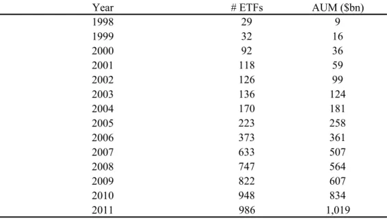
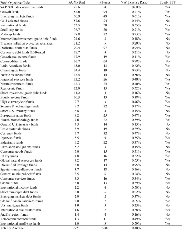
Our final sample consists of 1,146 distinct ETFs, with 1,065,832 daily observations with complete data from September 2, 1998 to March 31, 2011. Figure 1 illustrates the growth of ETFs over our sample period. At the start, the sample contains 20 ETFs, while at the end there are 986 ETFs with complete data. Table 1, Panel A, gives information on the growth of the assets in the ETF sector, showing that the average assets under management (AUM) in U.S. ETFs have grown from $9 billion in 29 ETFs during 1998 to over $1 trillion in 986 ETFs in March 2011. ETF growth in terms of assets and number of ETFs has picked up sharply after 2004. Panel B of Table 1, breaks down the ETFs in March 2011 by their Lipper objective code (for categories with more than $1 billion of AUM). The largest category by AUM contains the ETFs that track the S&P 500 with $95.6 billion in AUM and four ETFs, among which is the SPY that we study in the Flash-Crash analysis. The last column shows the fund objectives that have been included in the Equity ETF group in some of the regressions. From this group, we also exclude leveraged or short equity ETFs with the purpose of focusing on plain-vanilla equity ETFs.

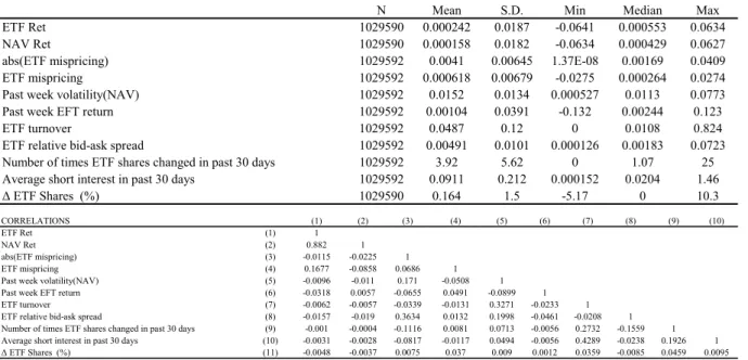
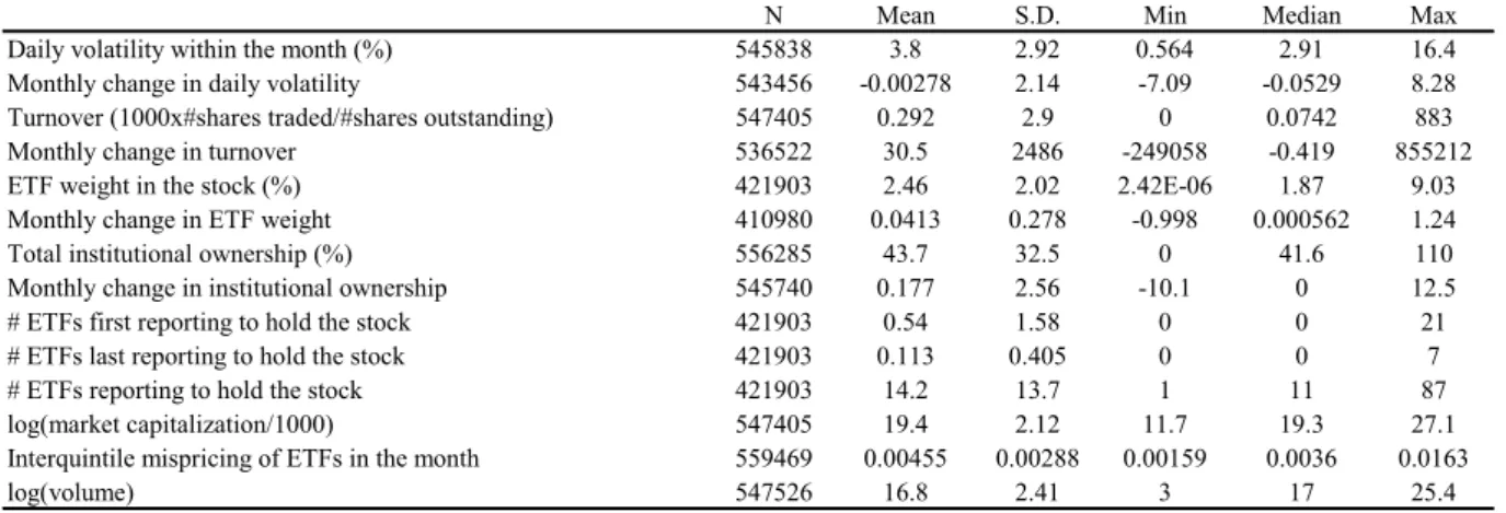
Table 2 reports summary statistics for the variables that are used in the regressions. We defer a description of these variables until we use them in the analysis.

3 ETFs and Arbitrage

3.1 Mechanics

of

Arbitrage

Exchange traded funds are investment companies that typically focus on one asset class, industry, or geographical area. Most ETFs track an index, very much like passive index funds. ETFs were first introduced in the late 1980s, but became more popular with issuance in January 1993 of the SPDR (known as “Spiders”, or Standard &Poor’s Depository Receipts), which is an ETF that tracks the S&P 500 (which we label “SPY” from its ticker). In 1995, another SPDR, the S&P MidCap 400 Index (MDY) was introduced, and since then the number exploded to more than 1,000 ETFs by the end of 2011. Other popular ETFs are the DIA which tracks the Dow Jones Industrials Average and QQQQ which tracks the Nasdaq-100. Since 2008, the Securities and Exchange Commission (SEC) allows actively-managed ETFs.

(8)

8

Similar to closed-end funds, retail and institutional investors can trade ETF shares in the secondary market.4 However, unlike closed-end funds, new ETFs shares can be created and redeemed. Since the price of ETF shares is determined by the demand and supply in the secondary market, it may diverge from the value of the underlying securities (the NAV). Some institutional investors (called “authorized participants,” AP), which are typically market makers or specialists, can trade bundles of ETF shares (called “creation units,” typically 50,000 shares) with the ETF sponsor. An AP can create new ETF shares by transferring the securities underlying the ETF to the ETF sponsor. Symmetrically, the AP can redeem ETF shares and receive the underlying securities in exchange. For some funds5 creations and redemptions of ETF shares can also happen in cash.

To illustrate the arbitrage process, we focus on the two cases of (i) ETF premium (the price of the ETF exceeds the NAV) and (ii) ETF discount (the ETF price is below the NAV). In the case of an ETF premium, APs have an incentive to buy the underlying securities, submit them to the ETF sponsor, and ask for newly created ETF shares in exchange. Then, the AP sells the new supply of ETF shares on the secondary market. This process generates a decline in the ETF price and an increase in the NAV, reducing and potentially eliminating the premium. In the case of an ETF discount, APs buy ETF units in the market and redeem them for the basket of underlying securities from the ETF sponsor. Then, the APs can sell the securities in the market.6 This generates positive price pressure for the ETF and negative pressure for the NAV, which reduces the discount.

Arbitrage can be undertaken by market participants who are not APs. Since both the underlying securities and ETFs are traded, investors can buy the inexpensive asset and short sell the more expensive one.7 For example, in case of an ETF premium, traders buy the underlying securities and short sell the ETF. They hold the positions until prices converge, at which point

4_{Barnhart and Rosenstein (2010) examine the effects of ETF introductions on the discount of closed-end funds and}

conclude that market participants treat ETFs as substitutions to closed-end funds.

5_{Creation and redemption for cash is especially common in ETFs on foreign assets, and where assets are illiquid,}

e.g., fixed income ETFs,

6_See_{http://ftalphaville.ft.com/blog/2009/03/12/53509/the-curious-case-of-etf-nav-deviations/}_{for a description of}

trading strategies by APs.

7_See

http://www.indexuniverse.com/publications/journalofindexes/joi-articles/4036-the-etf-index-pricing-relationship.html for a description of trading strategies that eliminate mispricing between ETFs and their underlying securities.

(9)

9

they cover their long and short positions to realize the arbitrage profit. Conversely, in the case of ETF discount, traders buy the ETF, and short sell the individual securities.

Finally, ETF prices can also be arbitraged against other ETFs (see Marshall, Nguyen, and Visaltanachoti 2010), or against futures contracts (see Richie, Daigler, and Gleason 2007).8_The latter case is relevant in our discussion of the Flash Crash, when the price drop in the E-mini futures on the S&P 500 was propagated to the ETFs on the same index via cross-market arbitrage.

To be precise, although these trading strategies involve claims on the same cash flows, they are not sensustricto arbitrages as they are not risk free. In particular, market frictions might

induce noise into the process. For example, execution may not be immediate, or shares may not be available for short selling, or mispricing can persist for longer than expected. In the remainder of the paper, we will talk about ETF arbitrage implying the broader definition of ‘risky arbitrage.’ Despite the fact that APs and many independent market participants engage in arbitrage activities, mispricing may still be present as a result of limits to arbitrage.

3.2 Time Series of ETF Mispricing

In this section, we explore the extent to which mispricing exists in the ETF market and link it to measures of limits to arbitrage. The goal is to provide the background for the following analysis which assumes that arbitrage activity is taking place between ETFs and their underlying securities. By showing that mispricing is related to the limits of arbitrage, in the time series and in the cross section, we indirectly infer that arbitrage is taking place when the constraints are not binding.

In Figure 2a, we plot the daily percentage mispricing for the SPY, the ETF tracking the S&P 500. The mispricing is defined as the ETF price minus the NAV divided by the ETF price. All these variables are measured at the day close. The SPY is the largest equity ETF, with a market capitalization of $90.965 billion in December 2010. The figure shows that the average mispricing shrank over time. This was possibly the result of the ETF market becoming more liquid, which reduced transaction costs for ETF arbitrage. There are multiple episodes in which

8_See_{http://seekingalpha.com/article/68064-arbitrage-opportunities-with-oil-etfs}_{for a description of a discussion of}

(10)

10

mispricing was sizeable. In particular, mispricing is larger during periods of market stress such the summer of 2007, and the fall of 2008, around the Lehman events. As an example, mispricing was 1% on October 22, 2008, and it was -1.2% on October 27, 2008. Note, further, that at times of high mispricing, the deviations from the NAV are both positive and negative, suggesting that the sign of the mispricing is less interesting than the magnitude of the mispricing as an indicator of limits of arbitrage. Overall, based on this graphical inspection, deviations from fundamental prices appear to be related to the overall liquidity in the market, which suggests a twofold interpretation. First, low market liquidity limits the profitability of ETF arbitrage due to the high transaction costs (see also Figure 2d). Second, low market liquidity can be a symptom of low funding liquidity (Brunnermeier and Pedersen 2009). In turn, a drop in funding liquidity implies that a reduced amount of capital is committed to ETF arbitrage allowing for a larger mispricing to persist.

In Figure 2b, we explore the evolution in the dispersion of mispricing for our entire sample of ETFs.9_{The chosen measure of dispersion is the interquartile range of mispricing} across the ETFs. Consistent with figure 2a, the dispersion of mispricing has a general downward trend, yet ETF mispricing increases across the board during periods of market stress (e.g., late 2002, summer 2007, early 2008, fall 2008, May 2010 (Flash Crash)).

Another interesting measure of mispricing is the net mispricing. We define net mispricing as the difference between the absolute value of the percentage mispricing and the percentage bid-ask spread for the ETF at the day close. This variable approximates the extent to which arbitraging the mispricing for a given ETF-day is profitable after transaction costs. In Figure 2c we report the fraction of ETFs with positive net mispricing in a given day. The figure shows that as the ETF industry expands, the fraction of mispriced ETFs increases. A likely explanation for this time-series relation is that bid-ask spreads shrink as the market becomes more familiar with ETFs and competition increases. As a consequence, a greater fraction of ETFs displays an absolute value of mispricing lying outside the bid-ask spread. Figure 2d confirms this conjecture. End-of-day spreads of ETFs decrease over time, but at times of market stress they increase.

9_{To gauge the evolution of the magnitude of mispricing over time for the cross-section of ETFs, we deem that the}

dispersion of the cross-sectional distribution is a more meaningful statistic than, say, the mean or the median. Because mispricing can be positive and negative, the latter statistics could provide the false impression that mispricing is low, when indeed for some funds it is very large and positive and for others it is very large and negative.

(11)

11

Especially, the bid-ask spreads increased dramatically during the crisis of 2008 paralleling the increase in mispricing observed in Figure 2b. Intuitively, as liquidity dried up, the bid-ask spread enlarged and arbitrageurs found it less profitable to trade on ETF mispricing, which widened as well. Incidentally, we note from Figure 2d that large drops of the ETF bid-ask spread occurred around August 2000 and February 2001. This is possibly the result of the decimalization of quotes on the Amex, where most ETFs were trading at the time (see Chen, Chou, and Chung 2008).

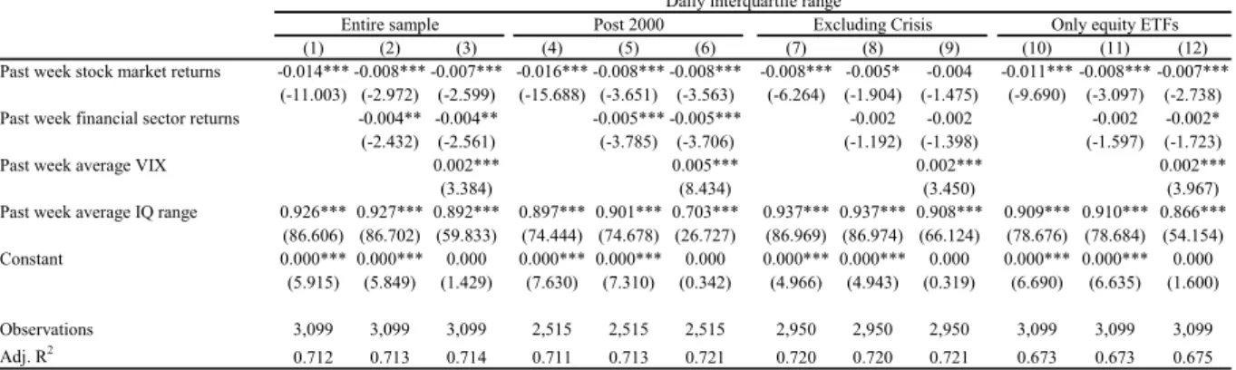
To obtain more systematic evidence on the determinants of mispricing we turn to regression analysis. In Table 3, we run time series regressions at the daily frequency where the dependent variables are summary measures of the daily ETF mispricing. The right-hand side variables are chosen to proxy for times where arbitrage capital is more likely to be scarce. Following, Hameed, Kang, and Viswanthan (2011), we use the stock market (value-weighted index) return in the prior five days to approximate the change in capital constraints in the market making sector. For the same purpose, we consider the prior-five-day return for the financial sector portfolio, which includes broker-dealers and excludes commercial banks (from Prof. Ken French’s forty-nine industry portfolios). Based on Nagel’s (2011) results that times of high VIX are related to a decrease in the supply of liquidity, we include the average level of the VIX in the prior five days. Finally, because mispricing is persistent and we want to focus on the daily innovations, we include the average mispricing in the prior five days. We consider different samples: Columns (1) to (3) present regressions using the entire sample of ETFs, Columns (4) to (6) use a sample that is limited to observations post-2000 (as transaction costs were substantially higher in the early years, as suggested by Figure 2d), Columns (7) to (9) exclude the peak of the financial crisis (the second half of 2008), which was arguably a ‘special’ time, and Columns (10) to (12) include only equity ETFs.

In Panel A of Table 3, the dependent variable is the interquartile range of ETF mispricing, which is plotted in Figure 2b. Consistent with a tightening of capital constraints on market makers and arbitrageurs, the estimates show an increase in the dispersion of mispricing following periods of low stock market returns. Even more convincing on the capital constraints channel, we find that mispricing increases following low past returns for the financial sector, controlling for the return on the stock market. Excluding the financial crisis (Columns (7) to (9)), we identify separate significant effects for the stock market and financial sector returns, and the

(12)

12

two variables are jointly significant. In general, the dispersion of mispricing increases with the VIX index.

To corroborate our results, in Table 3, Panel B, we consider an alternative dependent variable, the fraction of ETFs with positive net mispricing, which is plotted in Figure 2c. The panel shows that following periods of low financial sector returns the fraction of ETFs with positive net mispricing increases. The result is even stronger than in Panel A, as it holds also when the financial crisis is not in the sample. Interestingly, the regressions show that the fraction of ETFs with positive net mispricing decreases as the VIX index increases. In unreported analysis, we find that this effect takes place because bid-ask spreads expand at periods of high VIX (see also Figure 2d).

Overall, the results in this section present evidence that is consistent with the idea that ETF mispricing is larger at times in which arbitrageurs scale back their involvement in the market, either because they are losing capital or because of increased uncertainty.

3.3 The Cross Section of ETF Mispricing

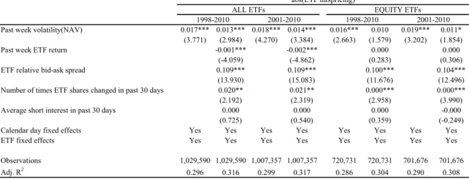
To provide additional evidence on the relation between ETF mispricing and limits to arbitrage, we exploit the cross-section of ETFs. Specifically, in Table 4 we regress the absolute value of mispricing (Panel A), or the signed value of mispricing (Panel B) on cross sectional determinants. Our sample is a panel of daily ETFs between 1998 and 2010. Time and fund fixed effects are included and standard errors are clustered at the fund level.

In Panel A, we find robust evidence that the magnitude of ETF mispricing increases with prior-five-day volatility of the NAV. This result suggests that the volatility in the underlying asset hinders arbitrageurs’ from taking advantage of the mispricing. Because we have time fixed effects, this measure of volatility is mostly capturing idiosyncratic volatility and supports the claim that idiosyncratic risk is a major limit to arbitrage (see, e.g., Pontiff 2006). The negative relation between absolute mispricing and the ETF prior-five day performance in Columns (2) and (4) may suggest that, if arbitrageurs are on average net long in the ETF, trading losses cause a decrease in the arbitrage capital committed to arbitrage ETF mispricing. This effect is not present in the sample of equity ETFs possibly because arbitrageurs do not have a positive net

(13)

13

exposure in this market. A strong result throughout the panel is the positive and significant relation between the ETF bid-ask spread and absolute mispricing, which speaks to the importance of transaction costs in limiting the profitability of arbitrage activity.

More direct evidence that arbitrage is taking place between the ETFs and the underlying securities comes from the positive link between the number of times that ETF shares outstanding change over the past thirty days and the absolute mispricing. As explained above, arbitrage by APs occurs via the creation/redemption of ETF units, which changes the number of shares outstanding. So, one can infer that more mispriced ETFs are characterized by more intense arbitrage activity. In this case, we are not capturing a causal relationship, but the fact that high mispricing attracts more arbitrage activity. Furthermore, our explanation relies on the fact that mispricing is positively autocorrelated (as seen in Table 5) so that if mispricing is high today it was likely high over the course of the prior month.

In Panel B, we focus on the signed mispricing. The goal is to identify variables that are related to the direction of mispricing, rather than to its absolute magnitude. The coefficient on prior week returns changes sign relative to Panel A. The likely mechanical explanation is that a run-up in ETF prices causes the ETF price to rise relative to the NAV. Note that the bid-ask spread loses its significance, which suggests that transaction costs operate to increase mispricing in both directions. Note that, consistent with our priors, there is a positive and significant coefficient on the average short interest in the ETF over the prior thirty days. Only when the mispricing has a positive sign, should arbitrageurs short sell the ETF and buy the underlying securities. So, it makes sense that short interest is significant in Panel B and not in Panel A. As in the case of the change in shares outstanding, we are not capturing a causal relation, but rather the fact that a positive mispricing attracts short sales. Again, our explanation relies on the positive autocorrelation of mispricing.

In sum, the evidence in this section shows that ETF mispricing is correlated with measures of limits to arbitrage, either in the form of constraints on arbitrage capital or in the form of holding and transaction costs. Furthermore, we have shown that mispricing attracts arbitrage activity, which shows up as changes in ETF shares outstanding and ETF short interest. Overall, we can conclude that arbitrage activity is tightly connected with ETF mispricing.

(14)

14

4 ETFs and Shock Transmission

After showing that arbitrage activity is taking place between ETFs and their underlying securities, we focus on the effects of arbitrage activity on stock returns and volatility. For a large part of this analysis, our focus is restricted to ETFs that trade in U.S. equity securities.

4.1 Effect on Returns

The conjecture that we explore in this paper is that arbitrage activity propagates non-fundamental shocks across markets. ETFs are an ideal candidate to shed light on this hypothesis because of the tight arbitrage relation that links them to the underlying securities. A liquidity shock occurring in the ETF market can cause a deviation of the ETF price from the NAV. Then, arbitrage activity may induce price pressure in the market for the underlying securities in the same direction as the initial shock in the ETF market.

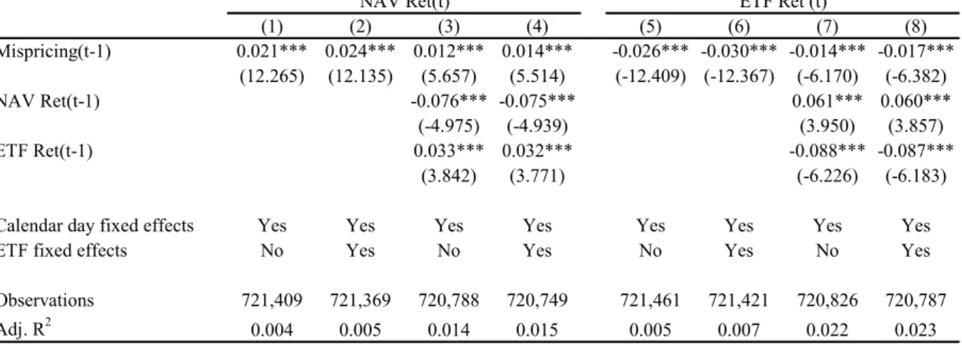
The first step in building this argument is to show that the underlying securities’ prices move in the same direction as the ETF mispricing. Using daily data after 2000 for equity ETFs, in Columns (1) to (4) of Table 5, we regress the day-t return on the NAV onto the mispricing in

day t – 1 and other controls. Date fixed effects are always included and standard errors are

clustered at the date level. Columns (1) and (2) show that, whether or not we control for fund fixed effects, the NAV return moves significantly in the same direction as the mispricing. This is consistent with the conjecture that arbitrage activity transmits a shock in the ETF market to the market of the underlying securities. The transmission occurs when there is a discrepancy between the ETF price and the NAV. As for the economic magnitude, for example, in Column (2) a one-standard deviation increase of mispricing in the previous day (0.619%) is associated with a 1 basis point (bp) increase in the daily return of the NAV. Given that the daily expected return for the average stock is of the order of magnitude of a few bps, the magnitude seems sizeable.10

There is another possible interpretation of this result. Price discovery may be taking place in the ETF first and the underlying securities’ prices may be following with some delay. For

10_{If we take an equity premium of about 6% annually and 250 trading days in a year, this corresponds to a daily}

(15)

15

example, upon the arrival of news, investors may be trading on this information in the ETF market because it is less expensive than trading in the basket of the underlying assets. In this case, we would observe a temporary mispricing which is then closed as the NAV catches up with a delay. To account for this channel, in Columns (3) and (4), we include the ETF return in day t –

1. This variable controls for the lead-lag relationship induced by early price discovery in the ETF market, to the extent that this effect plays out within the daily lag. Furthermore, to confound our identification, NAV returns may be autocorrelated so that a return on the NAV in day t – 1 is

related to the NAV return on day t as well as to the mispricing on the same day, as the NAV moves away from the ETF price on day t – 1. To filter this effect out, we also control for the

NAV return on day t – 1. Once these effects have been controlled for, the coefficient on

mispricing arguably captures the impact of mispricing arbitrage on the next day’s NAV. The relevant slope on mispricing in Columns (3) and (4) remains statistically significant. Quite intuitively, the magnitude is almost halved as we are filtering out the component of mispricing that results from day t – 1 movements both in the ETF price and the NAV, so that the residual

component of mispricing is the mispricing that has accumulated in days prior to t – 1.

The leg of the arbitrage that involves a trade in the ETF can bring about an ETF price movement of the opposite sign of the mispricing. So, to corroborate the conclusion that the estimated positive relation between mispricing and subsequent NAV returns is due to arbitrage, we run a regression of ETF return onto prior day mispricing. Columns (5) to (8) replicate the set of explanatory variables from the previous models. The negative and significant slope on mispricing is consistent with the movement expected if arbitrage activity is taking place. It is interesting to compare the magnitude of the coefficients, e.g., comparing Columns (4) and (8). The coefficients on the mispricing variable are similar, with opposite signs (0.014 vs. -0.017), suggesting that given a mispricing in day t – 1, both the NAV and ETF move to close the

mispricing on day t, almost by an equal amount.

As the effect of non-fundamental shocks to the ETF price is to generate mispricing, the results in Table 5 are consistent with the transmission of shocks from the ETF market to the prices of the underlying securities via arbitrage activity.

The mechanics of mispricing arbitrage implies that shock transmission from the ETF price to the price of underlying securities occurs via the creation/redemption of ETF shares.

(16)

16

When the ETF trades at a premium relative to the NAV, APs buy the underlying securities on the market, use them to create new ETF shares, which are then sold on the secondary market. This process puts upward pressure on the NAV and pushes down the ETF price. The opposite happens if the ETF trades at a discount. Therefore, we should expect changes in ETF share to be positively related to contemporaneous NAV returns.

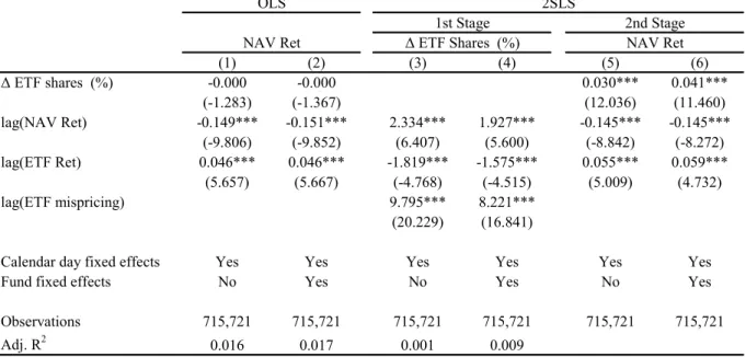
To find evidence of this effect, in Table 6, we regress daily stock returns onto the contemporaneous change in the number of ETF units, which is a proxy for arbitrage activity. The sample is restricted to daily equity-ETF returns starting in 2000 and standard errors are clustered at the date level. We include as control the lagged returns on the ETF and the NAV following the same logic as for Table 5. Columns (1) and (2) show that there is no significant relation between the two variables. This lack of significance is not surprising as ETF shares can change for reasons different from arbitrage. For example, during the process of introduction of a new ETF when new ETF shares are sold to the market, investors can shift their holdings from the underlying securities to the ETF, thus putting downward pressure in the price of the underlying assets. Also, an increase (decrease) in a particular ETF shares could be due to flows from (to) other similar ETFs that track similar index but have higher (lower) management expense fees, which would have zero net effect on the underlying securities. This effect would confound the effect of arbitrage, which is what we want to identify. To this purpose, we instrument the change in shares with the mispricing on the previous day in a two-stage least squares (2SLS) framework. The identifying assumption is that mispricing affects the NAV return on the next day only through the arbitrage activity, which induces the change in ETF shares outstanding. Columns (3) and (4) of Table 6 present the first stage, in which the change in shares is regressed on the mispricing. The slope on lagged mispricing is positive and significant as expected. These regressions suggest that an increase of one standard deviation in the mispricing is associated with an increase of about 1.4% in shares outstanding (Column (3)).

The second stage of the regression is presented in Columns (5) and (6) of Table 6. We are now able to identify a positive and significant relation between the instrumented change in ETF shares outstanding and the NAV return. This evidence suggests that indeed the returns of the underlying stocks move up when new shares are created to arbitrage away the existing mispricing. The opposite occurs when ETF shares are redeemed. As for the economic magnitude, a one-standard deviation increase (0.053 in Column (5) and 0.045 in Column (6)) in the

(17)

17

instrumented values of ΔETF shares is related to an increase of about 16 bps (Column (5), 18 bps in Column (6)) in the return of the underlying securities. This evidence complements the findings in Table 5 and suggests that arbitrage activity has an impact on the prices of the securities in the ETF basket.

4.2 Effect on Volatility

If non-fundamental shocks to ETF prices are passed down to the securities that compose the ETF basket, we should expect ETF ownership to increase stock volatility ceteris paribus.11

For this to happen, it has to be the case that arbitrage activity takes place between the ETF and the underlying assets. The results in Section 3 reveal that the intensity of arbitrage activity is time-varying as a function of limits to arbitrage. When arbitrage is constrained ETF mispricing is larger across the board.

Based on this intuition, we develop a test of the effect of ETF ownership on stock volatility, using the interquartile range of mispricing in a given time period as an inverse proxy for the intensity of arbitrage activity (see Figure 2b and Table 3). In practice, using stock-month level data between 1998 and 2010, we regress stock level volatility in a given month onto the interaction between the fraction of the stock capitalization held by ETFs in that month (ETF weight) and the average interquartile range of mispricing in the same month. We add the ETF weight and calendar month fixed effects as additional controls. Also, because ETF ownership could correlate with ownership by other institutional investor, while our focus is on ETFs, we also have controls for total institutional ownership and its interaction with the interquartile range of mispricing. Stock volume and capitalization are also included to control for unobservable stock characteristics which may attract ETF ownership, and stock fixed effects are sometimes considered for the same reason. Panel A of Table 7 has the estimates. Standard errors are clustered at the month level in Columns (1) and (3) and at the stock level in Columns (2) and (4). The results are supportive of the hypothesis that arbitrage activity increases the volatility of the underlying securities. The coefficients of the interaction between the average interquartile range and the ETF weight are negative in all columns. This suggests that at times in which arbitrage is

11_{Bradley and Litan (2011) raise similar concern in their testimony before the United States Senate Committee on}

(18)

18

tight, i.e. the average interquartile range of ETF mispricing is low, stocks with higher ETF holdings have higher volatility. From Column (1), a one-standard deviation increase in the interaction of ETF mispricing and ETF weight (0.016) decreases the daily volatility in the same month by about 15 bps.12 The mean daily volatility in our sample is about 3.8%, which suggests that the contribution of ETF ownership to daily volatility is not large on average, but can be sizeable for some stocks.

In Panel A of Table 7, we notice a negative relation between stock volatility and the level of ETF ownership. This reflects the fact that ETFs are typically created to track indexes, which tend to be comprised of larger and less volatile stocks. To get around this issue, in Panel B of Table 7 we look at the effect of a change in ETF ownership in month t on the change in stock

volatility between month t and month t + 1. Again, the idea is that an increase in ETF ownership

should bring about an increased exposure of the underlying stocks’ prices to non-fundamental shocks. The results are in Panel B of Table 7. Stock fixed effects are included in all specifications along with a control for a change in total institutional ownership. Standard errors are clustered at stock level and stock fixed effects are added to some of the specifications. From Columns (1) and (2), we note that an increase in ETF ownership of the stock raises the stock daily volatility in the following month, which is consistent with shock transmissions from the ETF to the underlying stocks. In terms of magnitude (from Column (1)), a 1% increase in the ETF weight raises daily volatility by 3 bps. Hence, for the stock with the median ETF ownership in December 2010 (4.3% ETF ownership), the daily volatility has increased over time as a consequence of ETF ownership by roughly 13 bps13 — which amounts to 3.4% of daily stock volatility.14 For the stock at the 90th percentile of ETF ownership in December 2010 (ETF ownership of 7.9%), the cumulative increase in volatility is approximately 24 bps, or 6.3% of daily volatility.

Naturally, one would expect smaller stocks to be more sensitive to shock transmission from the ETFs due to their lower liquidity. In Columns (3) and (4) of Panel B, Table 7, we add an interaction between a small stock indicator (capitalization the below the CRSP median in the month) and the change in ETF weight. As expected, the regressions show that the magnitude of

12_{0.016 × 9.3 = 0.15} 13_{4.3 × 3 bps = 12.9 bps}

(19)

19

the increase in volatility is significantly larger for smaller stocks. Actually it appears that the entire effect of the change in ETF weight plays out among these smaller stocks, as the baseline effect is statistically insignificant.

In the third test of the effect of ETF ownership on stock volatility, we focus on ETFs that begin or stop holding a stock. Under our hypothesis, an increase in the number of ETFs that own the stock should increase stock volatility because of the increased exposure to the non-fundamental shocks coming from the ETF market. The opposite happens if ETFs stop holding the stock. The number of ETFs holding the stock is drawn from the ETF investment company filings with the SEC, and which are available in Thomson-Reuters Mutual Fund Ownership database.

In Columns (1) and (2) of Panel C, Table 7, we test this conjecture. The dependent variable is the same as in Panel B, the change in volatility between month t and month t +1. The

number of ETFs is measured at month t. We include as controls the change in total institutional

ownership (as reported in the institutional 13F filings), logged market capitalization, volatility in month t, turnover in month t, and the number of ETFs that hold the stock in month t, as our focus

is on the change (positive or negative) in this number. Standard errors are clustered at the stock level. Consistent with our conjecture, the regressions show that monthly volatility increases when additional ETFs start holding the stock, and it decreases when ETFs stop including the stock in their basket, holding constant the total number of ETFs that own the stock. Coverage by one additional ETF increases the daily volatility in the next month by 0.016% to 0.019%. A withdrawal of an ETF decreases the daily volatility in the next month by 0.038% to 0.047%.

If this volatility effects occurs via the arbitrage activity induced by ETF mispricing, we should observe increased trading in the stock as new ETFs cover the stock. In Columns (3) and (4) we test this conjecture. The dependent variable is the change in turnover between months t

and t +1. The explanatory variables are the same as in Columns (1) and (2). The results are

consistent with our prior, as the change in turnover is significantly related to positive and negative changes in ETFs covering the stock. As more ETFs cover the stock, turnover increases, keeping constant the total number of ETFs owning the stock. Stock turnover decreases when ETFs stop holding the stock.

(20)

20

Overall, the results in this section suggest that ETFs have a significant impact on the prices of the stocks in their basket. This effect results from arbitrage activity which propagates shocks in the ETF price to the prices of the underlying securities. As a result ETF ownership increases volatility of the underlying stocks.

5 Evidence from the Flash Crash

The events in the U.S. stock market in May 6, 2010 (the “Flash Crash”) drew the attention of the media and of regulators to ETFs. On that day, the S&P 500 plunged nearly 6% within minutes and recovered by the end of the day (see Figure 3a). According to CFTC and SEC report (2010), which summarized their findings about the Flash Crash, the price decline began in the futures market, when a large institutional investor sold S&P 500 E-mini futures contracts at an increasing rate, which as a consequence led to a liquidity dry up in the futures market. At the present time, a full account on how the liquidity problem in the futures market led to a crash in the equity market is still missing.15

In this section we test whether arbitrage trading on ETFs contributed to transmitting the shock from the futures market to the equity market. The idea is that ETFs tracking the S&P 500 were arbitraged against two types of assets: the futures contracts (S&P 500 E-minis),16 and the basket of underlying stocks (the S&P 500). The liquidity shock hit initially the futures contract. Consistent with the anecdotal evidence (see the CFTC and SEC 2010 preliminary and final reports), we conjecture that the arbitrage relation between the futures market and the ETF market led the ETFs to decline as well. Then, an arbitrage relation between ETFs and the underlying stocks led to the transmission of the liquidity shock to the equity market.

We begin by eye-balling the S&P 500 index (the NAV), the S&P 500 E-mini futures, and the SPY (the largest ETF on the S&P 500) in Figures 3b and 3c in the time period leading to trough of the three series, which occurred at about 14:45:45. The figure shows that the E-mini was leading the decline in price, then the ETF followed, and the NAV moved last. In most of the

15_{Among traded securities, ETFs were among the ones that declined the most. The prevailing explanation among}

industry practitioners (e.g., Borkovec, Domowitz, Serbin, and Yegerman 2010) for this fact is that market makers for ETF pulled out of the market after suffering severe losses. As a result market liquidity dried up, leading to further decline in prices.

16_{Richie, Daigler, and Gleason (2007) describe the process in which the arbitrage between S&P 500 futures and the}

(21)

21

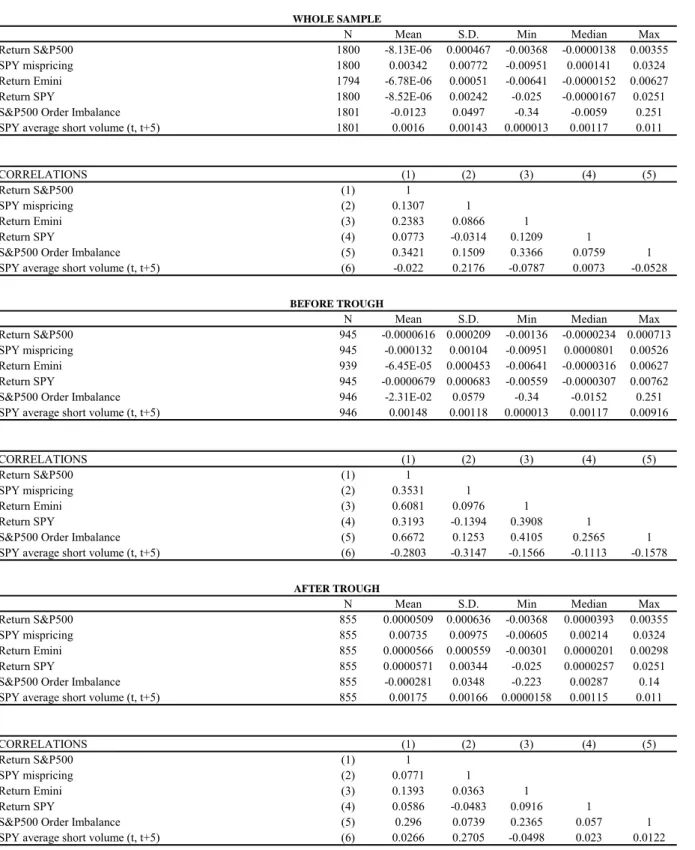
seconds in the two charts, during the way down, the NAV is located above the ETF. This suggests an explanation in which the futures price decline induced arbitrageurs to sell ETFs and by futures. Then, the ETF traded at a discount relative to the NAV, which made it profitable to buy ETFs and sell the basket of underlying securities, causing part of the decline in the S&P 500. To test this relation more formally, we turn to a time-series regression framework, using one-second level data for the period between 14:30 and 15:00. In Table 8, Panel A, Column (1), we regress the returns on the S&P 500 index on the SPY mispricing in the previous second. The positive coefficient suggests that the S&P 500 declined more strongly following seconds in which the mispricing was negative, i.e., the S&P 500 was above the SPY. The magnitude of the coefficient can be interpreted as follows: a one-standard deviation decrease in the SPY mispricing (i.e., the SPY is lower than S&P 500 index) is associated with a 0.6 bps decline in the S&P 500 in the following second.

Two potential non-mutually exclusive explanations can cause this relation. The first one is the arbitrage relation we have discussed so far: market participants buy the ETF and short sell the NAV. The second explanation is based on price discovery: market participants observe the prices of the futures contract and of the ETF, and use them as guidelines for the true valuation of the S&P 500 (Cespa and Foucault 2011). To disentangle the two stories, we control for the lagged returns of the S&P 500, the lagged returns of the SPY, and the lagged returns of the e-mini S&P 500 futures contract (Column (2)). The regression shows that the magnitude and the significance of the SPY mispricing remain intact even when these variables are included. Also, we control for longer horizon changes in the prices of these variables in Column (3). The coefficient of interest declines in magnitude, but it remains statistically significant. We conclude that our arbitrage hypothesis is a viable complementary explanation to the price discovery channel.

In Columns (4) to (9) we split the sample to the pre-trough period (pre 14:45:45), and post-trough period (post 14:45:45). The results show that the arbitrage relation between the ETF mispricing and the returns on the NAV remains strong and has similar magnitude for both periods.

To further establish the conjecture that ETFs served as a conduit for transmitting the shock in the futures market to the equities market through the mechanism of arbitrage, we

(22)

22

explore the determinants of the order imbalance on the S&P 500. This variable is compute as the dollar value of buy trades minus the dollar value of sell trades in the second, scaled by the total market capitalization (the variable is measured as % of market capitalization and multiplied by 1000). In Table 8, Panel B, we regress the S&P 500 order imbalance on the lagged ETF mispricing (Column (1)), as well as lagged cumulative returns (Column (2)). The regressions show that order imbalance on the S&P 500 is positively correlated with the extent of the ETF mispricing. At times in which the SPY mispricing is low (i.e., the price of the S&P 500 is above the SPY), order imbalance is low, meaning that there are more selling orders for the S&P 500 than buy orders. Hence, these findings further solidify the conclusion that price pressure on the S&P 500 developed as a result of arbitrage between the SPY and the S&P 500.

Finally, ETF mispricing arbitrage involves selling the ETF whenever its price is above the NAV. During the Flash Crash, this occurred after the trough. So, if arbitrage was occurring we should observe a significantly positive relation between the short volume in the ETF and the mispricing, only when the mispricing was positive, that is, after the trough. Panel C of Table 8 provides evidence which is consistent with this conjecture. The relationship is positive and significant in Columns (5) and (6), that is, after the market had hit the bottom. The data for intraday short volume in the SPY comes from Arca, and we average this variable over the five seconds between t and t + 5 to reduce noise. The standard errors are adjusted to account for

autocorrelation using the Newey and West (1987) estimator with five lags. The evidence from Panel C is also suggestive that arbitrage activity was occurring to take advantage of the SPY mispricing.

To summarize, the results in this section are consistent with the idea that the arbitrage relation between ETFs and the underlying securities, and between ETFs and the futures market, contributed to the propagation of the Flash Crash from the futures market to the equity market.

6 Conclusion

The paper shows that arbitrage activity can lead to the propagation of non-fundamental shocks across assets that are tied by an arbitrage relation. We present several pieces of evidence on this mechanism in the ETF market. First, we show that arbitrage activity is taking place between ETFs and their underlying securities. Second, we show that coverage of stocks by ETFs

(23)

23

is associated with increased volatility and turnover, especially in small stocks. Third, we present evidence from the Flash Crash demonstrating that ETFs served as a conduit for shock transmission from the futures market to the equity market.

Our results provide a novel and provocative interpretation of the role of arbitrage in financial markets. Arbitrage does not only adjust prices of mispriced securities, but also it can move the price of securities that are correctly priced. Thus, the greater resources dedicated to arbitrage mispricing away do not necessarily improve the quality of pricing.

Related to this, our findings complement the recent evidence about comovement of stocks and indices (e.g., Barberis, Shleifer, and Wurgler 2005). We suggest that arbitrage activity can propagate non-fundamental shocks and induce heightened volatility and correlation. The changes in the second moments could potentially reflect a deterioration of the degree of price efficiency. This topic deserves further theoretical and empirical research.

Finally, our results should be of interest to regulators. The evidence in the paper suggests that ETFs, a relatively new instrument that grew tremendously in the last few years, may increase the risk of contagion in financial markets by transmitting non-fundamental shocks. Our study of the Flash Crash of May 6, 2010, is a notable example in this direction.

(24)

24

References

Amihud, Yakov, 2002, Illiquidity and Stock Returns: Cross-Section and Time-Series Effects,

Journal of Financial Markets 5(1), 31-56.

Anton, Miguel and Christopher Polk, 2010, Connected Stocks, Working Paper, London School of Economics.

Barnhart, Scott W., and Stuart Rosenstein, 2010, Exchange-Traded Fund Introductions and Closed-End Fund Discounts and Volume, Financial Review 45(4), 973-994.

Barberis, Nicholas, Andrei Shleifer, and Jeffrey Wurgler. 2005, Comovement, Journal of

Financial Economics 75(2), 283-317.

Basak, Suleyman and Anna Pavlova, 2010, Asset Prices and Institutional Investors, Working Paper, London Business School.

Borkovec, Milan, Ian Domowitz, Vitaly Serbin, and Henry Yegerman, 2010, Liquidity and Price Discovery in Exchange-Traded Funds, Investment Technology Group Report.

Bradley, Harold, and Robert E. Litan, 2011, ETFs and the Present Danger to Capital Formation, Testimony before the United States Senate Committee on Banking, Housing, and Urban Affairs. October 19th_{, 2011.Brunnermeier, Markus K., and Lasse H. Pedersen, 2009, Market Liquidity} and Funding Liquidity, Review of Financial Studies 22, 2201-2238.

Cella, Cristina, Andrew Ellul, and Mariassunta Giannetti, 2011, Investors’ Horizons and the Amplification of Market Shocks, Working Paper, Stockholm School of Economics and Indiana University.

Cespa, Giovanni, and Thierry Foucault, 2011, Learning from Prices, Liquidity Spillovers, and Endogenous Market Segmentation, Working paper, HEC Paris.

Chang, Yen-Cheng and Harrison G. Hong, 2011, Rules and Regression Discontinuities in Asset Markets, Working Paper, Princeton University.

Chen, Wei-Peng, Robin K. Chou, and Huimin Chung, 2008, Decimalization and the ETFs and Futures Pricing Efficiency, Journal of Futures Markets 29(2), 157-178.

Commodity Futures Trading Commission and Securities & Exchange Commission, 2010, Findings regarding the market events of May 6, 2010,

www.sec.gov/news/studies/2010/marketevents-report.pdf

Coval, Joshua, and Erik Stafford, 2007, Asset Fire Sales (and Purchases) in Equity Markets,

Journal of Financial Economics 86(2), 479-512.

Crawford, Steve S., James Hansen and Richard Price, 2010,CRSP Portfolio Methodology and the Effect on Excess Returns, Working Paper, Rice University.

Greenwood, Robin, and David Thesmar, 2011, Stock price fragility. Journal of Financial

Economics 102(3), 471-490.

Gromb, Denis, and Dimitri Vayanos, 2010, Limits of Arbitrage: The State of the Theory, Annual

Review of Financial Economics 2, 251–275.

Hameed, Allaudeen, Wenjin Kang, and S. Viswanathan, 2010, Stock Market Declines and Liquidity, Journal of Finance 65(1), 257-293.

(25)

25

Jiang, Guohua, Charles M. C. Lee, and Yi Zhang, 2005, Information Uncertainty and Expected Returns, Review of Accounting Studies 10, 185-221.

Lee, Charles M. C., and Mark J. Ready, 1991, Inferring trade direction from intraday data,

Journal of Finance 46(2), 733-746.

Lou, Dong, 2011, A Flow-Based Explanation of Returns Predictability, Working Paper, London School of Economics.

Marshall, Ben R., Nhut H. Nguyen, and Nuttawat Visaltanachoti, 2010, ETF Arbitrage, Working Paper, Massey University.

Nagel, Stefan, 2010, Evaporating Liquidity, Working Paper, Stanford University.

Pontiff, Jeffrey, 2006, Costly arbitrage and the myth of idiosyncratic risk, Journal of Accounting and Economics, 42, 35-52.

Ramaswamy, Srichander, 2011, Market Structures and Systemic Risks of Exchange-Traded Funds, Working Paper, Bank of International Settlements.

Richie, Nivine, Robert Daigler, and Kimberly C. Gleason, 2007, Index Arbitrage between Futures and ETFs: Evidence on the limits to arbitrage from S&P 500 Futures and SPDRs, XXXX Trainor, William J. Jr., 2010, Do Leveraged ETFs Increase Volatility? Technology and

Investment 1(3), 215-220.

Vayanos, Dimitri, and Paul Woolley, 2011, Fund Flows and Asset Prices: A Baseline Model, Working Paper, London School of Economics.

Wurgler, Jeffrey, 2010, On the Economic Consequences of Index-Linked Investing, Working Paper, New York University.

(26)

26

Appendix: List of Variables

ETF variables Description Data Sources

ETF Return ETF Closing Price and ETF distributions

made during the period, divided by ETF closing price in the previous period

CRSP, Compustat, OptionMetrics

NAV Return Change in the Net Asset Value of ETF

portfolio securities. NAV is computed as the fair market value of all ETF security

holdings, divided by ETF shares outstanding

CRSP Mutual Fund Database, Lipper

ETF Mispricing Difference between ETF Price and ETF

NAV. Positive (Negative) ETF mispricing is referred to as ETF Premium (Discount).

CRSP, Compustat, OptionMetrics, CRSP MFDB and Lipper

NAV Volatility Standard deviation of the NAV return CRSP Mutual Fund

Database, Lipper ETF relative bid-ask spread Difference between closing ask and closing

ask, relative to closing midpoint

Equity ETF Identifying ETFs with the majority of

portfolio in equity securities using Lipper (CRSP MFDB) and Morningstar investment objective codes. Non-Equity ETFs include Bond, commodities, derivatives (e.g. short bias, leveraged, etc.) and other asset classes.

CRSP Mutual Fund Database, Lipper, Morningstar

ETF Turnover ETF Trading Volume during the period,

scaled by period end ETF shares outstanding

ETF AUM ETF market value calculated as day end

shares outstanding multiplied by closing ETF price

CRSP, Compustat, OptionMetrics ETF Short Interest Ratio in the past

30 days End of month and mid-month short interest shares (adjusted) scaled by day end shares outstanding

Compustat

Cross Sectional Measures Description Data Sources

Daily interquartile range interquartile range of mispricing across all ETFs in each time period used as an inverse proxy for the intensity of arbitrage activity

CRSP, Compustat, OptionMetrics, CRSP MFDB and Lipper Daily fraction of ETFs with

positive net mispricing Number of ETFs with ETF price above the NAV, scaled by the total number of ETFs. Fraction > 0.5 is when most ETFs exhibit premiums possibly due to positive demand shocks

CRSP, Compustat, OptionMetrics, CRSP MFDB and Lipper

(27)

27

Appendix: List of Variables (Cont.)

Stock Level Variables Description Data Sources

Daily volatility within the month (%)

Standard deviation of daily returns during the month

CRSP

Turnover Period Volume scaled by period-end shares

outstanding, after adjusting both volume and shares outstanding to splits and similar events.

CRSP

ETF weight in the stock (%) Total shares owned by ETF scaled by total shares outstanding, for each common stock. ETF holdings are extracted from their most recent holdings reports (N-CSR, N-CSRS, and N-Qs) that they are required to file pursuant to the Investment Company Act of 1940, and which are collected by Thomson-Reuters Mutual Fund Ownership Database

Thomson-Reuters Mutual Fund Ownership Data

Total institutional ownership (%) Total shares owned by institutions divided

by stock shares outstanding. Thomson-Reuters 13F Data # ETFs first reporting to hold the

stock

Using ETF mutual fund holdings report to determine the number of new ETFs that started reporting during that month and that they hold this stock.

# ETFs last reporting to hold the stock

The number of ETFs that own this stock and that will never report their holdings

afterwards. Conditional analysis on those two variables allows a better identification, by focusing on the increase in weights that coincide with inception of new ETFs that will hold the stock (and vice versa for stocks with decreasing ETF weights because of closing ETFs).

# ETFs reporting to hold the stock The breadth of ownership by ETF which is the number of ETFs that reported their holdings in this stock, in the most recent ETF mutual fund ownership filings.

(28)

28

Appendix: List of Variables (Cont.)

Intraday Variables Description Data Sources

S&P500 Return Using TAQ and CME trade data for individual ETFs, common stocks, and E-minis, volume weighted average prices are constructed at the second intervals using all valid trades in each second. Intraday returns are then computed each second as the price in second t divided by the price in second t-1, minus one. If there are no trades in a particular second, the return is set to zero. S&P 500 returns are computed by averaging the returns of individual components each second, using as weights, the market value of S&P 500 components in day -1

TAQ

SPY Return TAQ

E-Mini Return CME

S&P500 Stocks Average Order

Imbalance After computing the second-level buy sell imbalance as fraction of stock market value for each stock, a weighted average order imbalance is aggregated across all S&P500 components, similar to intraday return computation.

TAQ

SPY Average Short Volume Using ARCA RegSho data, short volume are aggregated each second and then divided by total shares outstanding.

ARCA

(29)

29

Table 1. ETF Sample Description

The table presents the distribution of ETFs in our sample. Panel A has the number of ETFs at year-end and the average monthly total assets under management (AUM, in $billion) of ETFs over the year. Panel B presents summary statistics on AUM (in $billion), the number of funds, and a value-weighted expense ratio by objective code as of end of March 2011 (for funds for which the objective code is not missing). The last column of Panel B shows whether the fund is included in the equity funds’ sample.

Panel A: ETF Statistics, by Year

Year # ETFs AUM ($bn)

1998 29 9 1999 32 16 2000 92 36 2001 118 59 2002 126 99 2003 136 124 2004 170 181 2005 223 258 2006 373 361 2007 633 507 2008 747 564 2009 822 607 2010 948 834 2011 986 1,019

(30)

30

Table 1. ETF Sample Description (Cont.) Panel B: ETF Statistics, by Objective Code

Fund Objective Code AUM ($bn) # Funds VW Expense Ratio Equity ETF

S&P 500 index objective funds 95.6 4 0.09% Yes

Growth funds 82.6 94 0.21% Yes

Emerging markets funds 70.9 49 0.61% Yes

Gold oriented funds 57.6 24 0.44% No

International funds 53.5 38 0.35% Yes

Small-cap funds 36.7 30 0.21% Yes

Mid-cap funds 28.8 32 0.23% Yes

Intermediate investment grade debt funds 24.6 8 0.18% No

Treasury inflation protected securities 21.2 5 0.20% No

Dedicated short bias funds 20.4 97 0.94% No

Corporate debt funds BBB-rated 18.7 8 0.21% No

Growth and income funds 17.9 19 0.11% Yes

Commodities funds 16.7 64 0.78% No

Latin American funds 15.0 13 0.62% Yes

China region funds 14.4 19 0.73% No

Pacific ex Japan funds 13.4 14 0.56% No

Financial services funds 13.2 26 0.40% Yes

Natural resources funds 12.3 25 0.40% Yes

Real estate funds 12.0 15 0.32% Yes

Short investment grade debt funds 11.2 4 0.16% No

Equity income funds 10.3 13 0.38% Yes

High current yield funds 9.7 3 0.46% Yes

Science & technology funds 9.2 32 0.37% Yes

Short U.S. treasury funds 8.8 4 0.15% No

European region funds 8.2 25 0.47% Yes

Health/biotechnology funds 7.6 22 0.39% Yes

General U.S. treasury funds 7.5 14 0.15% No

Basic materials funds 5.9 19 0.39% No

Currency funds 5.7 32 0.47% No

Japanese funds 5.5 9 0.55% Yes

Industrials funds 5.2 22 0.37% Yes

Ultra-short obligations funds 5.2 3 0.15% No

Consumer goods funds 5.0 15 0.31% Yes

Utility funds 4.8 16 0.32% Yes

Global natural resources funds 4.2 17 0.55% Yes

Diversified leverage funds 3.8 14 0.95% No

Specialty/miscellaneous funds 3.7 18 0.56% No

General municipal debt funds 3.5 6 0.24% No

Consumer services funds 3.5 16 0.34% Yes

Global funds 3.0 13 0.39% Yes

International income funds 2.2 4 0.50% No

Short municipal debt funds 2.0 6 0.22% No

Emerging markets debt funds 2.0 2 0.57% No

Global financial services funds 2.0 7 0.65% Yes

U.S. mortgage funds 1.9 3 0.25% No

International real estate funds 1.6 7 0.58% Yes

Pacific region funds 1.4 4 0.16% No

Telecommunication funds 1.3 11 0.49% Yes

International small-cap funds 1.0 3 0.59% Yes

(31)

31

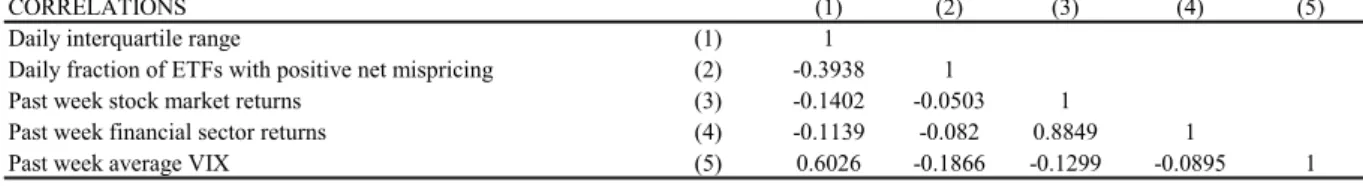
Table 2. Summary Statistics

The table presents summary statistics about the variables used in the regressions. Panel A shows summary statistics of ETF data aggregated at a daily level. Panel B shows summary statistics about the dataset that is at the ETF-day level. Panel C presents summary statistics for data at the stock-month level. Panel D presents second-level data used at the Flash Crash analysis.

Panel A: Time-series, ETF-level, analysis

N Mean S.D. Min Median Max

Daily interquartile range 3104 0.00504 0.00371 0.00129 0.00402 0.0351

Daily fraction of ETFs with positive net mispricing 3104 0.325 0.163 0 0.362 0.723

Past week stock market returns 4509 0.00195 0.0255 -0.186 0.00358 0.2

Past week financial sector returns 4509 0.00309 0.043 -0.272 0.00457 0.373

Past week average VIX 4509 0.207 0.0857 0.0968 0.196 0.729

CORRELATIONS (1) (2) (3) (4) (5)

Daily interquartile range (1) 1

Daily fraction of ETFs with positive net mispricing (2) -0.388 1

Past week stock market returns (3) -0.1353 -0.0308 1

Past week financial sector returns (4) -0.117 -0.0636 0.8865 1