Dynamic Linkages in the Pairs (GBP/EUR, USD/EUR) and (GBP/USD, EUR/USD): How Do They Change During a Day?

Dynamic Linkages in the Pairs (GBP/EUR,

USD/EUR) and (GBP/USD, EUR/USD):

How Do They Change During a Day?

Małgorzata Doman

, Ryszard Doman

Abstract

In the paper, we document how conditional dependencies observed in the FOREX market change during a trading day. The analysis is performed for the pairs (GBP/EUR, USD/EUR) and (GBP/USD, EUR/USD) of exchange rates. We consider daily returns calculated using the exchange rates quoted at different hours of a day. The dynamics of the dependencies is modeled by means of 3-regime Markov 3-regime switching copula models, and the strength of the linkages is described using dynamic Spearman’s rho and the dynamic coefficients of tail dependence. The established approach allows us to monitor the changes in the dependence structure.

Keywords: exchange rates, FOREX, linkages, copula, Markov regime switching, Spearman’s rho, volatility, tail dependence, crisis

JEL Classification: G15, C58, G01, C32

∗_{Poznań University of Economics; e-mail: malgorzata.doman@ue.poznan.pl} †_{Adam Mickiewicz University in Poznań; e-mail: rydoman@amu.edu.pl}

1

Introduction

In the paper, we document that the dynamics of linkages between the exchange rates for the pairs (GBP/EUR, USD/EUR) and (GBP/USD, EUR/USD) depends on time of a trading day. The analysis is based on daily returns calculated using the exchange rates quoted at 11 fixed hours of a day. To describe changes in a pattern of the linkages we apply 3-regime Markov regime switching copula models, and the strength of the dependencies is described using dynamic Spearman’s rho and tail dependence coefficients.

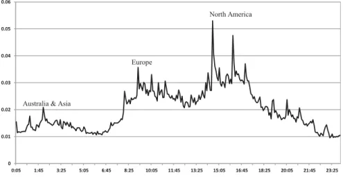
The FOREX market is open 24 hours a day, with the exception of weekends. Trades between the FOREX participants are conducted through electronic communication networks and phone networks in various markets around the world. While some regional markets are closed, the other are open and the trade lasts. Trading hours of several regional markets overlap what results in more active FOREX trading during some periods. Figure 1 presents the periodic daily pattern observed in 5-minute returns of the exchange rate EUR/USD. The plot is obtained by calculating the average absolute value of the returns corresponding to each 5-minute segment. It is easy to observe that during a day there are three phases of higher volatility and thereby with higher market activity. The maxima visible in Figure 1 indicate the periods of the highest activity of traders from three main FOREX regions: Australia and Asia, Europe, and North America. The idea of our analysis comes from a conjecture that this pattern of changing activity should generate different patterns of conditional dependencies for daily returns built on exchange rates quoted at different times of a day. This is the reason why we perform our analysis of dependencies using daily returns calculated based on quotations from selected fixed hours of a day. Considering daily returns calculated in such a way seems to be quite natural in some circumstances. For instance, the daily returns calculated based on the quotations from 2:00 CET are strongly influenced by the activity of the Asian traders, and those corresponding to 9:00 CET can be considered as a result of decisions taken by the European traders. For investors from different continents different currencies are of importance, which should be reflected in the dynamics of dependencies. To the best of our knowledge, there are no earlier studies concerning the problem of changes in linkages in the FOREX market that take the proposed approach.

In Table 1, we show trading hours for the stock markets in the considered regions. Approximately, these periods are consistent with the periods of the most active trade in regional FOREX markets.

Our choice to model the dependencies for the pairs (GBP/EUR, USD/EUR) and (GBP/USD, EUR/USD) is connected with the idea of currency co-movement promoted by Eun and Lai (2004) and Eun et al. (2013). The investigation of co-movement in currency market is complicated because in order to describe the linkages between two currencies it is necessary to consider their exchange rates. Since the latter are calculated against a third currency, the results of the analysis strongly depend on the choice of it. Eun and Lai (2004) suggest that the exchange rates against the euro

Figure 1: EUR/USD. The daily periodic pattern in 5-minute returns (Central European Time). Calculations based on the observations from the period: November 11, 2011 — January 31, 2014 0 0.01 0.02 0.03 0.04 0.05 0.06 0:05 1:45 3:25 5:05 6:45 8:25 10:05 11:45 13:25 15:05 16:45 18:25 20:05 21:45 23:25 Europe North America

Australia & Asia

Table 1: A rough chart of trading hours for stock markets

CET 0 1 2 3 4 5 6 7 8 9 10 11 12 13 14 15 16 17 18 19 20 21 22 23 Australia Japan Singapore India Europe USA

should be used to describe linkages with the U.S. dollar, and, similarly, the exchange rates against the U.S. dollar should be applied to explain linkages with the euro. According to their philosophy, our analysis shows how the impacts of the U.S. dollar and the euro on the British pound change during the trading day in the FOREX market.

Our investigation covers the period from March 2, 2005 to January 31, 2014, and thus includes the long periods of financial crises and turmoil in global financial market. We are interested in possible changes in the structure of conditional dependencies which could be caused by these events. For this reason, our analysis is based on 3-regime Markov regime switching copula models, which are a tool flexible enough to capture qualitative and/or quantitative changes of the linkages in currency market. Applying this approach, we can measure not only the average conditional dependence using dynamic Spearman’s rho coefficients, but, additionally, the obtained estimates of tail dependence coefficients enable us to get a deeper insight into the pattern of

the dependencies between extreme observations. In particular, due to applying the Markov regime switching copula models we are able to thoroughly trace temporal changes in the impact of the global currencies on the British pound during the period under scrutiny.

The results of our research are thus twofold. First, we show how the dynamic linkages between the GBP and the USD or the EUR are changing during the trading day. The second group of our results deals with those changes in the daily pattern of the dependencies which are caused by observed market events.

2

Copula-based dependence measures

It is well documented (McNeil et al. 2005) that outside the class of elliptical distributions (e.g. multivariate normal or multivariate Student’s t) an adequate approach to measuring dependence between random variables should use the concept of a copula. A bivariate copula is a mapping C : [0,1]×[0,1] → [0,1] from the unit square into the unit interval, which is a distribution function whose marginal distributions are standard uniform. The importance of copulas follows from a theorem by Sklar (1959). It states that if (X, Y) is a 2-dimensional random vector with joint distribution H and marginal distributions F and G then for some copula C the following formula holds:

H(x, y) =C(F(x), G(y)). (1)

If F and G are continuous, the copulaC is unique. It is called the copula of H or (X, Y), and can be represented as

C(u, v) =H(F←(u), G←(v)) (2)

for u, v ∈ [0,1], where F←(u) = inf{x : F(x) ≥ u}. It follows from (1) that by means of copula the marginals and the dependence structure can be separated. Thus, it makes sense to interpret the copula C as the dependence structure of the vector (X, Y).

The simplest copula is the one corresponding to independence of marginal distributions. It is defined by CΠ_{(u, v) = uv. In this paper we will also use the}

Gaussian, Joe-Clayton, and rotated Joe-Clayton copulas. They are defined as follows:

C_ρGauss(u, v) = Φρ Φ−1(u),Φ−1(v), (3) C_κ,γJ−C(u, v) = 1− 1−[1−(1−u)κ]−γ+ [1−(1−v)κ]−γ−1 −1/γ1/κ , (4) C_κ,γJ−C_r90(u, v) =v−C_κ,γJ−C(1−u, v). (5)

In formula (3), Φρ denotes the distribution function of a standard 2-dimensional

normal distribution function.

The parameters of the Joe-Clayton copula (4) are assumed to satisfy the conditions:

κ ≥ 1, γ > 0. For κ = 1, the Joe-Clayton copula becomes the Clayton copula

CClayton

γ . In the limit caseγ = 0, the Clayton copula approaches the independent

copulaCΠ_{(Nelsen 2006). The rotated version of the Joe-Clayton copula, C}J−C_r90

κ,γ ,

is applied to modeling negative dependence, which is impossible using the copula

Cκ,γJ−C.

An absolutely continuous copulaC possesses the densitycdefined by

c(u, v) =∂

2_{C(u, v)}

∂u∂v . (6)

IfH is an absolutely continuous distribution function with the copulaC, the density

c is related to the joint density functionhby the following canonical representation:

h(x, y) =c(F(x), G(y))f(x)g(y), (7)

whereF andGare the marginal distribution functions, andf andgare the marginal density functions.

Copula-based dependence measures are the ones that depend only on the copula of a random vector (X, Y). In particular, such measures are invariant with respect to strictly increasing transformations of the variablesXorY.In the case of non-elliptical random vectors they should be used instead of the linear correlation coefficient in order to avoid potential pitfalls (see, McNeil et al. 2005). An example of a copula-based dependence measure, which is used in the empirical part of this paper, is Spearman’s rho. It is defined as

ρS(X, Y) =ρ(F(x), G(y)), (8)

where F andG are the distribution functions of the variablesX andY, respectively (McNeil et al. 2005). If (X, Y) is a vector whose components have continuous distribution functions, andC is its copula, then

ρS(X, Y) =ρC = 12

Z Z

[0,1]2

C(u, v)dudv−3 (9)

(Nelsen 2006). In the case of the Gaussian copula, CGauss

ρ , Spearman’s rho equals 6

πarcsin 1

2ρ

(McNeil et al. 2005). There is no explicit formula for Spearman’s rho for the Clayton and Joe-Clayton copulas, so in this case one has to compute it numerically using (9). Spearman’s rhos for the copula CJ−C_r90

κ,γ and Cκ,γJ−C differ

only by the sign.

In financial applications, it is often very important to know whether two variables behave similarly when their extreme values occur. Such phenomena can be described in probabilistic terms by coefficients of tail dependence (see, Joe 1997). If X and

upper tail dependence is defined as

λU,U = lim

q→1−P(Y > G

←_{(q)|X > F}←_{(q)), (10)}

provided a limit λU,U ∈ [0,1] exists. Analogously, the coefficient of lower tail

dependence is defined as

λL,L= lim

q→0+P(Y ≤G

←_{(q)|X ≤F}←_{(q)), (11)}

provided that a limitλL,L∈[0,1] exists. IfλU,U ∈(0,1] (λL,L∈(0,1]), thenX and Y are said to exhibit upper (lower) tail dependence. Upper (lower) tail dependence assesses the likelihood to observe a large (low) value ofY given a large (low) value of

X. The coefficients of tail dependence are copula-based dependence measures: ifC is the copula linkingX andY then

λL,L= lim q→0+ C(q, q) q , (12) λU,U= lim q→0+ ˆ C(q, q) q . (13)

where ˆC(u, v) =u+v−1 +C(1−u,1−v). The Gaussian copula does not exhibit tail dependence: λU,U =λL,L = 0 (McNeil et al. 2005). In the case of the Joe-Clayton

copula,λU,U= 2−21/κandλL,L= 2−1/γ (Patton 2006), which means that upper and

lower tail dependence coefficients are independent of each other.

When the components of the random vector (X, Y) display negative dependence the notion of negative tail dependence should be introduced. We define the coefficients of negative tail dependence,λU,LandλL,U, by the following formulas:

λU,L= lim q→0+P(Y ≤G ←_{(q)|X > F}←_{(1−q)), (14)} λL,U = lim q→1−P(Y > G ←_{(q)|X ≤F}←_{(1−q)), (15)}

provided that the limits exist. It can be directly shown that the coefficients of negative tail dependence depend solely on the copulaC of the random vector (X, Y):

λU,L= lim q→0+ q−C(1−q, q) q , (16) λL,U = lim q→0+ q−C(q,1−q) q . (17)

Moreover, formulas (5), (12), (13), (16) and (17) show that for the rotated Joe-Clayton copulaCJ−C_r90

κ,γ the following holds: λU,L Cκ,γJ−C_r90 =λL,L Cκ,γJ−C = 2−1γ_{, (18)} λL,U Cκ,γJ−C_r90 =λU,U Cκ,γJ−C = 2−2κ1_{. (19)}

3

Markov regime switching copula models

When modeling time-varying joint conditional distributions of bivariate returns, the evolution of the conditional copulaCthas to be specified. Usually, the functional form

of the conditional copula is fixed, but its parameters evolve through time (Patton 2004, 2006), or it is assumed that there are regimes in each of which a fixed copula prevails, and they switch according to some Markov chain (Garcia and Tsafack 2011). In the present paper, we follow the latter approach. Thus in the applied Markov regime switching copula model (MRSC model) the joint conditional distribution of the vectorrt= (r1,t, r2,t) has the following form

rt|Ωt−1∼CSt(F1,t(·), F2,t(·)|Ωt−1) (20)

where St is a homogeneous Markov chain with state space {1,2,3}. The

parameters of the MRSC model are the parameters of univariate models for marginal distributions (ARMA-GARCH), the parameters of copulas C1, C2

and C3, and the transition probabilities, pij = P(St=j|St−1=i), (i, j) ∈ {(1,1),(2,2),(3,3),(1,2),(2,1),(3,2)}.

The parameters of the model have been estimated by the maximum likelihood method. The main by-products of the estimation are the conditional probabilities

P(St=j|Ωt−1) and P(St = j|Ωt), j = 1,2,3, which are calculated by means of

Hamilton’s filter (Hamilton 1994):

P(St=j|Ωt−1) = 3 X i=1 pijP(St−1=i|Ωt−1), (21) P(St=j|Ωt) = cj(ut|St=j,Ωt−1)P(St=j|Ωt−1) 3 P i=1 ci(ut|St=i,Ωt−1)P(St=i|Ωt−1) , (22) where p13= 1−p11−p12,p23= 1−p21−p22,p31= 1−p31−p33,ut= (u1,t, u2,t)0, u1,t=F1,t(r1,t), u2,t=F2,t(r2,t), (23)

andcj(·|St=j,Ωt−1) is the density of the conditional copula coupling the conditional

marginal distributions in regimej,j= 1,2,3. The maximized log-likelihood function has the form

L = T P t=1 ln 3 P j=1 cj ut|St=j,Ωt−1; ˜θj P St=j|Ωt−1; ˜θj ! + + T P t=1 ln (f1,t(r1,t|Ωt−1;θ1)) + T P t=1 ln (f2,t(r2,t|Ωt−1;θ2)) , (24)

wheref1,tandf2,tare the density functions corresponding toF1,tandF2,t, fitted using

When presenting the empirical results, we use the so-called smoothed probabilities. They are calculated from the predicted and filtered probabilities by using the backward recursion: P(St=j|ΩT) =P(St=j|Ωt) 3 X i=1 pjiP(St+1=i|ΩT) P(St+1=i|Ωt) , t=T−1, . . . ,1, (25)

whereT denotes the length of the sample.

The models are estimated by the two-step maximum likelihood method. Thus, first we fit univariate ARMA-GARCH models to the return data. Then, the obtained standardized residuals are transformed to uniform variates, using the theoretical cumulative distribution functions. After that, the Markov regime switching copula models are fitted and estimates of dynamic Spearman’s rho and the lower and upper tail coefficients and the coefficients of negative tail dependence are calculated using the smoothed probabilities.

The above approach to estimating copula-based models has an advantage that it is computationally tractable at a moderate cost of the loss of full efficiency (Patton 2012, 2013). As an alternative approach, Bayesian inference should be mentioned (see e.g. Min and Czado 2010, Almeida and Czado 2012, and references therein). The latter includes uncertainty of the parameter estimates and can deliver credible intervals for the time-varying point estimates of Spearman’s rho.

4

The Model Confidence Set

The Model Confidence Set (MCS) methodology was introduced by Hansen et al. (2003). It was originally designed for selecting the best volatility forecasting models. Its applications, however, are not limited to evaluation of models. Equally well, it can be used to compare the means of two or more populations. The MCS procedure allows to select in a set of models a subset consisting of models which are better than the others in terms of some specified criterion. To be precise, for some collection

M0_{of models, the MCS procedure produces a subset ˆM}∗

1−α of M0, which contains

the subsetM∗ _{of superior models with a given confidence level 1−α. The collection} M0 _{can be any finite set of objects indexed by i = 1, . . . , m}

0. Suppose they are

evaluated in terms of a loss function that assigns to the objecti in periodt the loss

Li,t, t = 1, . . . , n. If the relative performance is defined as dij,t ≡ Li,t −Lj,t for

i, j ∈ M0 _{and the meanµ}

ij ≡E(dij,t) is finite and does not depend on t, then the

set of superior objects is defined by

M∗_≡

i∈ M0_{: µ}

ij ≤0 for allj∈ M0 .

The MCS procedure uses an equivalence testδM to test the hypothesis

at levelαfor anyM ⊂ M0_{. WhenH}

0,Mis rejected, an elimination ruleeMis applied

to identify the object ofM that is to be removed fromM. Consequently, the MCS is based on the following steps:

Step 0: Set initiallyM=M0_.

Step 1: TestH0,M at significance levelαusing δM.

Step 2: IfH0,M is not rejected, set ˆM∗1−α =M, otherwise useeM to eliminate

an object fromMand repeat the procedure beginning with Step 1.

It is proved in Hansen et al. (2011) that under some standard requirements for the equivalence test and the elimination rule it holds that

lim inf n→∞P M∗⊂Mˆ∗_1−α≥1−α, (26) lim n→∞P i∈Mˆ∗_1−α= 0 for alli /∈ M∗, (27) lim n→∞P M∗_{= ˆM}∗ 1−α

= 1 ifM∗_{consists of a single model. (28)}

The MCS p-values are defined as follows. If PH0,Mi denotes thep-value associated

with the null hypothesis H0,Mi (with convention that PH0,Mm0 = 1), then the MCS p-value for modeleMj ∈ M

0_{is defined as ˆp}

eMj ≡maxi≤jPH0,Mi.

The null hypothesisH0,Mcan be tested using traditional quadratic-form statistics or

multiplet-statistics (see, Hansen et al. 2011). In this paper, we apply thet-statistic

TR,Mdefined as TR,M= max i,j∈M|tij|, (29) where tij= ¯ dij q vˆar d¯ij fori, j∈ M, (30)

and ¯dij = n−1Pn_t=1dij,t. Because of the presence of nuisance parameters, the

asymptotic distribution of the statistic TR,M is nonstandard. The bootstrap

implementation of the MCS procedure involving this statistic is described in Appendix B of the paper by Hansen et al. (2003). The estimated bootstrap distribution of

TR,M, under the null hypothesis, is given by the empirical distribution of

T_b,R∗ = max i,j∈M |d¯∗_b,ij−d¯ij| q c var ¯dij , (31) where ¯d∗_b,ij = _n1Pn

t=1dij,τ_bt is the bootstrap resample average, and var ¯c dij = = _B1 PB b=1 ¯ d∗_b,ij−d¯ij 2

. For generating B resamples, the block bootstrap is used. Thep-value ofH0,Mis given by

PH0,M= 1 B B X b=1 1Tb,R∗ > TR,M . (32)

In the present paper, we apply the MCS procedure to compare the means of exchange rate volatilities, and the averages of strength of linkages between exchange rates, measured by means of Spearman’s rho.

5

The data

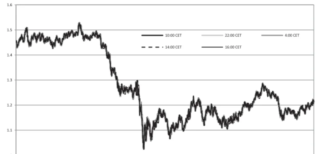
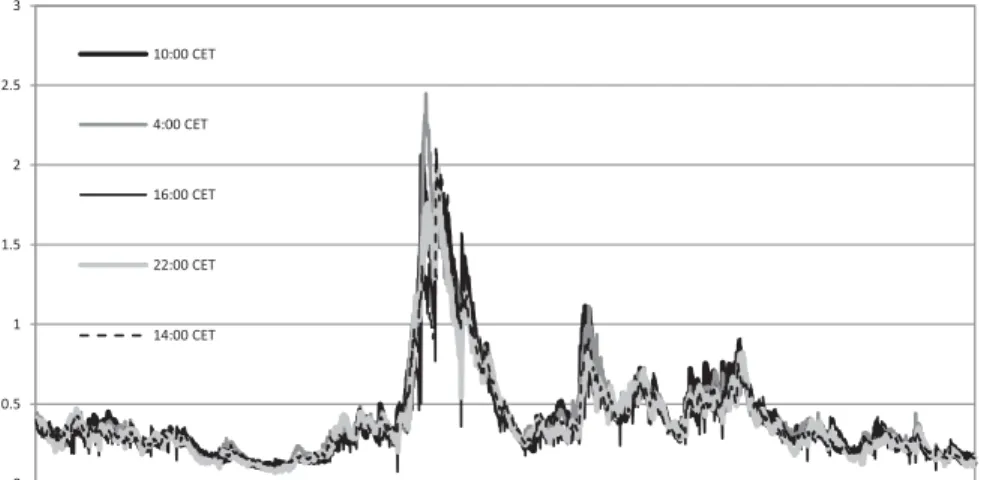
We investigate the exchange rates GBP/USD, GBP/EUR and EUR/USD. As it is established in the practice of FX markets, the symbol X/Y means the price of a unit of the currency X in units of the currency Y. The analysis is performed for the daily percentage logarithmic returns, which are separately calculated based on exchange rates quoted at 11 fixed hours of a day: 2:00 CET, 4:00 CET, 6:00 CET , . . . ,22:00 CET. The period under scrutiny is from March 2, 2005 to January 31, 2014 (2317 daily observations for each of the selected hours). The exchange rate series were obtained from the service Stooq. The plots in Figure 2 present the quotations, over the period under scrutiny, of the exchange rate GBP/EUR at indicated hours of a day. The fluctuations of the quotations of the GBP/EUR at the selected hours of the same day are not very strong, and similar behavior has been observed in the case of the other analyzed exchange rates.

Figure 2: The quotations of the exchange rate GBP/EUR at 4.00, 10.00, 14.00, 16.00. 22.00 CET 1 1.1 1.2 1.3 1.4 1.5 1.6 2005-03-01 2005-12-06 2006-09-12 2007-06-21 2008-04-01 2009-01-08 2009-10-15 2010-07-26 2011-05-02 2012-02-06 2012-11-12 2013-08-21 10:00 CET 22:00 CET 4:00 CET 14:00 CET 16:00 CET

6

Analysis of volatility and dependencies

To investigate dependencies between the analyzed exchange rates, we use 3-regime Markov switching copula models. This allows us to describe different types of dependence and capture temporal changes in the linkages of the GBP with the USD or the EUR.

As mentioned in Section 3, we applied a 2-step estimation procedure. First, we fitted a univariate ARMA-GARCH model to each of the investigated return series. As usually in the case of very liquid assets, the fitted models are mostly simple GARCH or GJR-GARCH with a Student’stor skewed Student’stdistribution for the innovations (Tsay 2010). The standardized residuals from the fitted ARMA-GARCH models were examined for consistency with the assumed distributional properties and serial independence. Next, they were transformed by means of the theoretical cumulative distribution functions into the series of the form (23), and the MRSC models were fitted by the maximum likelihood method, using the first summand in (24). We considered copulas from various families including those allowing to capture negative dependence. In the final choice we followed the results of the information criteria and the likelihood ratio tests performed where they were applicable. The estimation was done using G@RCH 6.0 package (Laurent 2009) and the Matlab software.

The first part of our results concerns the dynamics of volatility. Due to space limitations, we do not report here full results of the estimation of univariate models. Table 2 contains the types of GARCH models fitted to the analyzed data. In Figures 3-8, the corresponding volatility estimates are shown.

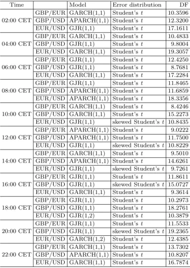
Table 2 shows that the dynamics of the daily exchange rate returns is changing over the day. Interesting things are appearance and disappearance of asymmetry in the data and changes in the number of degree of freedom (DF) in Student’s t distribution. A lower DF value means more frequent occurrence of outliers in the return process. This indicates higher market sensitivity on new information and is connected with more active trading. In the case of the EUR/USD, the highest DF values are observed from 2:00 CET to 8:00 CET. This is a time period when the European and the U.S. markets are closed. At the same time, we observe the lowest DF values for the GBP/USD. This means that for Asian traders the latter exchange rate is more important than the former. The GBP/EUR is the most heavily traded when the European markets are open (9:00 CET – 17:00 CET). There are only four cases with skewed Student’s

t distribution (negative asymmetry) for the innovations: EUR/USD (at 10:00 CET and 14:00 CET) and GBP/USD (at 16:00 CET and 20:00 CET).

When the fitted models are GJR-GARCH or APARCH, we meet another type of asymmetry connected with the so-called leverage effect (see, Tsay 2010). From Tables 1 and 2 it is easy to see that in the case of the GBP/EUR returns this type of asymmetry is produced by joint activity of Asian markets (in particular Indian markets) and the U.S. markets. The GBP/USD daily returns show asymmetric behavior for all the considered hours with the exception of 10:00 CET (joint impact of Asian and European markets). The best model for the EUR/USD data is mostly a

GARCH(1,1). The asymmetric phenomena are present at 2:00 CET, 8:00 CET, 12:00 CET (model), 10.00 CET (distribution) and 14:00 CET (model and distribution).

Table 2: Types of GARCH models fitted to daily returns calculated for data quoted at the selected hours

Time Model Error distribution DF

02:00 CET

GBP/EUR GARCH(1,1) Student’st 10.3596 GBP/USD APARCH(1,1) Student’st 12.3200 EUR/USD GJR(1,1) Student’st 17.1611 04:00 CET

GBP/EUR GARCH(1,1) Student’st 10.4833 GBP/USD GJR(1,1) Student’st 9.8004 EUR/USD GARCH(1,1) Student’st 19.3057 06:00 CET

GBP/EUR GJR(1,1) Student’st 12.4250 GBP/USD GJR(1,1) Student’st 8.7681 EUR/USD GARCH(1,1) Student’st 17.2284 08:00 CET

GBP/EUR GJR(1,1) Student’st 11.8465 GBP/USD APARCH(1,1) Student’st 11.6859 EUR/USD APARCH(1,1) Student’st 18.3356 10:00 CET

GBP/EUR GARCH(1,1) Student’st 8.4246 GBP/USD GARCH(1,1) Student’st 15.2273 EUR/USD GJR(1,1) skewed Student’st 10.8435 12:00 CET

GBP/EUR APARCH(1,1) Student’st 9.0222 GBP/USD APARCH(1,1) Student’st 11.7500 EUR/USD GJR(1,1) skewed Student’st 10.8229 14:00 CET

GBP/EUR GARCH(1,1) Student’st 9.5010 GBP/USD APARCH(1,1) Student’st 14.6261 EUR/USD GJR(1,1) skewed Student’st 9.7261 16:00 CET

GBP/EUR GJR(1,1) Student’st 11.8611 GBP/USD GJR(1,1) skewed Student’st 15.0727 EUR/USD GARCH(1,1) Student’st 9.3614 18:00 CET GBP/EUR GJR(1,1) Student’st 10.2973 GBP/USD GJR(1,1) Student’st 18.2761 EUR/USD GJR(1,2) Student’st 10.3879 20:00 CET GBP/EUR GJR(1,1) Student’st 11.5533 GBP/USD GJR(1,1) skewed Student’st 19.2365 EUR/USD GARCH(1,2) Student’st 12.4385 22:00 CET

GBP/EUR GARCH(1,1) Student’st 13.7302 GBP/USD APARCH(1,1) Student’st 10.8207 EUR/USD GARCH(1,1) Student’st 16.7874

The models described in Table 2 are simple, but they indicate some changes in the dynamics of volatility when different hours of a day are considered. These diverse models, however, give very similar volatility estimates. This is clearly visible in Figures 3-5 presenting volatility estimates for the exchange rates quoted at 4:00 CET, 10:00 CET, 14:00 CET, 16:00 CET and 22:00 CET. All the plots show a well-known

volatility pattern. The explosion of volatility corresponds in each case to the short period during the subprime crisis encompassing the bankruptcy of Lehman Brothers. The main observation is that the daily volatility estimates corresponding to different hours do not differ significantly. This impression is confirmed by the plots in Figures 6-8 presenting a synthetic view on the volatility estimates.

The surfaces presented in Figures 6-8 show that generally the level of volatility remains almost unchanged across the selected hours of a day. Some fluctuations, however, are observed during turmoil periods – the strongest during the subprime crisis and weaker in time of the Eurozone crisis. This indicates a higher market sensibility on information during the crisis period.

The main part of our analysis deals with the question about the changes in the conditional dependence structure connected with the activity of different regional markets. In Table 3 we present the types of all fitted MRSC models, and in Tables 4-6, examples of parameter estimates are given. In the case of the pair (GBP/USD, EUR/USD) we do not observe tail dependence. The fitted models are 3 or 2-regime MRSC ones with two Gaussian copulas and the independence copula in the case where regime 3 appears. The number of regimes changes depending on the considered hour of a day. The dynamics of linkages between the GBP/EUR and USD/EUR is more complicated. Usually, in one of the regimes the Joe-Clayton copula prevails, indicating the presence of lower and upper tail dependencies. The only exceptions are 8:00 CET (before European markets opening) and 22:00 CET (the U.S. market closing).

Table 3: The types of MRSC models fitted to daily returns calculated for data quoted at the selected hours

Time 02:00 04:00 06:00 08:00 10:00 12:00 14:00 16:00 18:00 20:00 22:00 GBP/EUR-G-G-JC JC-JC GBP/EUR-G-G-JC G-G JC-JC G-G-JC G-G-JC G-G-JC G-G-JC G-G-JC G-G USD/EUR GBP/USD-G-G-Π G-G G-G G-G-Π G-G G-G G-G-Π G-G-Π G-G G-G-Π G-G-Π EUR/USD

Tables 4-6 present parameter estimates for MRSC models fitted to daily returns calculated for the data quoted at 16:00 CET, 10:00 CET, and 6:00 CET. The chosen models fit the data well. Gaussian copulas describing dependence in different regimes differ by their correlation coefficients, indicating stronger or weaker dependence. The matrices of transition probabilities show that regimes are distinguished properly. The observed dependencies are strong, so there was no doubt about the choice of the best model.

Figure 9 presents estimates for dynamic Spearman’s rho for (GBP/USD, EUR/USD). The dynamics changes with the considered hours of a day. The most stable linkages correspond to 4:00 CET and 10:00 CET. Spectacular drops in the strength of dependence occur during the periods of turmoil in financial markets. An interesting observation is that during the periods of crisis the value of Spearman’s rho decreases even to 0, indicating temporary conditional independence. The surface of dynamic

Figure 3: GBP/EUR. Daily volatility estimates corresponding to different hours 0 0.5 1 1.5 2 2.5 2005-03-02 2006-04-26 2007-06-22 2008-08-20 2009-10-16 2010-12-14 2012-02-07 2013-04-04 10.00 CET 22.00 CET 4.00 CET 16.00 CET 14.00 CET

Figure 4: GBP/USD. Daily volatility estimates corresponding to different hours

0 0.5 1 1.5 2 2.5 3 3.5 2005-03-02 2005-12-07 2006-09-13 2007-06-22 2008-04-02 2009-01-09 2009-10-16 2010-07-27 2011-05-03 2012-02-07 2012-11-13 2013-08-22 10:00 CET 4:00 CET 22:00 CET 16:00 CET 14:00 CET

Spearman’s rhos in Figure 10 confirms the above remarks.

The MRSC models fitted to (GBP/EUR, USD/EUR) are more complicated than those for (GBP/USD, EUR/USD). However, the dynamics of Spearman’s rho presented in Figures 11-12 seems to be less sensitive on markets events. The Spearman’s rho estimates are lower but more stable. The periods of sharp increase are connected with crises in the USA and in the Eurozone. The plot in Figure 12, however, shows that even during calm periods conditional dependence between GBP/EUR and

Figure 5: EUR/USD. Daily volatility estimates corresponding to different hours 0 0.5 1 1.5 2 2.5 3 2005-03-02 2005-12-07 2006-09-13 2007-06-22 2008-04-02 2009-01-09 2009-10-16 2010-07-27 2011-05-03 2012-02-07 2012-11-13 2013-08-22 10:00 CET 4:00 CET 16:00 CET 22:00 CET 14:00 CET

Figure 6: GBP/EUR. Surface of volatilities

USD/EUR changes with the considered hours of a day.

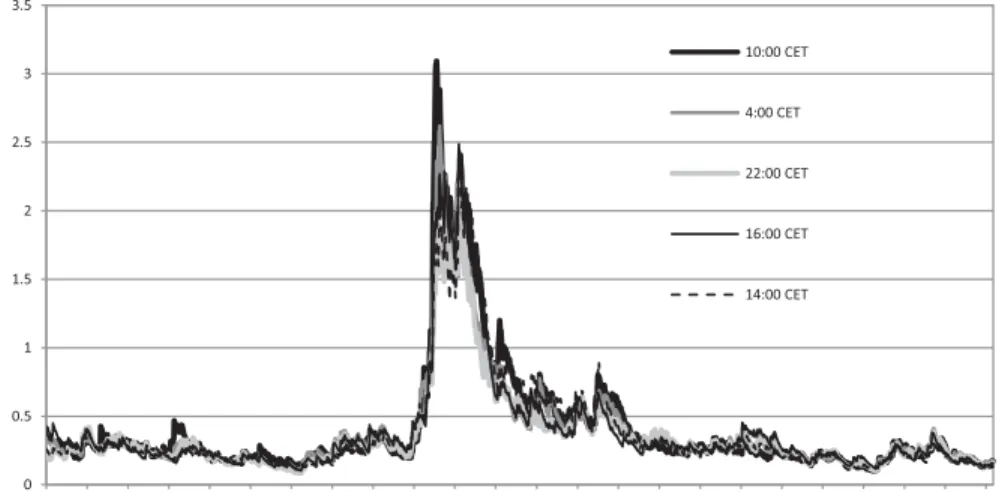
In Figure 13 we present estimates of the dynamic coefficients of lower tail dependence for the pair (GBP/EUR, USD/EUR). The dynamics is similar to that visible in Figure 11. The main observation is that lower tail dependence appears in crisis periods (the subprime crisis and the Eurozone crisis).

In the last part of the analysis we use the MCS methodology to compare the averages of strength of linkages measured by means of Spearman’s rho obtained for pairs of daily returns corresponding to the considered hours of a day. A similar comparison

Figure 7: GBP/USD. Surface of volatilities

Figure 8: EUR/USD. Surface of volatilities

is performed for the averages of the considered exchange rate volatilities.

Tables 7-8 contain the orderings of the considered hours of a day according to the average of dynamic Spearman’s rho (or the average of volatility) obtained with the MCS procedure applied sequentially. This means that after each run, the series constituting the MCS are excluded. Each block in the corresponding column (Tables 7-8) contains a model confidence set, i.e. a set of hours for which the analyzed averages are statistically indistinguishable. All the MCSs (with significance levelα= 0.1) have been estimated using the package MulCom by Hansen and Lunde (2010) written in

Table 4: Parameter estimates for MRSC models fitted to daily returns calculated for data quoted at 16:00 CET

GBP-EUR GBP-USD

GBP/USD

Regime 1 Regime 2 Regime 3 GBP/EURRegime 1 Regime 2 Regime 3

EUR/USD USD/EUR

Copula CGauss

ρ CρGauss CΠ Copula CρGauss CρGauss CJ oe

−Clayton κ,γ ρ 0.6317 (0.0242) (00.8019.0098) ρ (00.2828.0270) (00.6396.0211) κ κ 3.5480 (0.4410) γ γ 2.4248 (0.6465) Transition probabilities Transition probabilities Regime 1 0.9925 0.0030 0.0045 Regime 1 0.9987 0.0013 0.0000 Regime 2 0.0030 0.9970 0.000 Regime 2 0.0021 0.9941 0.0038 Regime 3 0.0755 0.0000 0.9245 Regime 3 0.0001 0.0057 0.9422

Table 5: Parameter estimates for MRSC models fitted to daily returns calculated for data quoted at 10:00 CET

GBP-EUR GBP-USD

GBP/USD

Regime 1 Regime 2 GBP/EUR Regime 1 Regime 2

EUR/USD USD/EUR Copula CGauss ρ CρGauss Copula CJ oe −Clayton κ,γ CJ oe −Clayton κ,γ ρ 0.5649 (0.0310) (00.7885.0152) ρ κ κ 1.2956 (0.0392) (01.8873.1025) γ γ 0.1302 (0.0359) (00.7871.1053) Transition probabilities Transition probabilities Regime 1 0.9838 0.0162 Regime 1 0.9988 0.0012 Regime 2 0.0129 0.9871 Regime 2 0.0034 0.9966

Ox (Doornik 2006).

The highest level of dependence between the GBP/USD and EUR/USD is observed when the European markets are open. In the case of (GBP/EUR, USD/EUR), the strongest linkages are produced by Asian markets. For each of the considered hours the average of dynamic Spearman’s rho for (GBP/USD, EUR/USD) turned out to

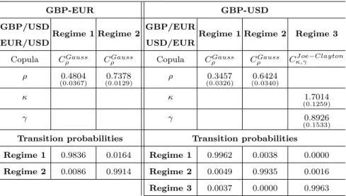
Table 6: Parameter estimates for MRSC models fitted to daily returns calculated for data quoted at 6.00 CET

GBP-EUR GBP-USD

GBP/USD

Regime 1 Regime 2 GBP/EURRegime 1 Regime 2 Regime 3

EUR/USD USD/EUR

Copula CGauss

ρ CρGauss Copula CρGauss CρGauss CJ oe

−Clayton κ,γ ρ 0.4804 (0.0367) (00.7378.0129) ρ (00.3457.0326) (00.6424.0340) κ κ 1.7014 (0.1259) γ γ 0.8926 (0.1533) Transition probabilities Transition probabilities Regime 1 0.9836 0.0164 Regime 1 0.9962 0.0038 0.0000 Regime 2 0.0086 0.9914 Regime 2 0.0049 0.9935 0.0016 Regime 3 0.0037 0.0000 0.9963

be significantly higher than that for (GBP/EUR, USD/EUR). There are, however, some periods and hours when of dynamic Spearman’s rho estimates show stronger dependence for the pair (GBP/EUR, USD/EUR) (Figure 14).

Figure 9: Dynamic Spearman’s rhos for (GBP/USD, EUR/USD)

0 0.1 0.2 0.3 0.4 0.5 0.6 0.7 0.8 0.9 2005-03-02 2005-12-07 2006-09-13 2007-06-22 2008-04-02 2009-01-09 2009-10-16 2010-07-27 2011-05-03 2012-02-07 2012-11-13 2013-08-22 4:00 CET 10:00 CET 14:00 CET 16:00 CET 22:00 CET

Figure 10: Surface of dynamic Spearman’s rhos for (GBP/USD, EUR/USD)

Figure 11: Dynamic Spearman’s rhos for (GBP/EUR, USD/EUR)

0 0.1 0.2 0.3 0.4 0.5 0.6 0.7 0.8 0.9 1 2005-03-02 2005-12-07 2006-09-13 2007-06-22 2008-04-02 2009-01-09 2009-10-16 2010-07-27 2011-05-03 2012-02-07 2012-11-13 2013-08-22 4.00 CET 10.00 CET 14.00 CET 16.00 CET 22.00 CET

to be little surprising. The higher averages of volatility are connected with activity of Asian markets. In agreement with what we expected, the highest volatility of the GBP/EUR appears during the trade in European markets. In general, however, the results presented in Table 8 are consistent with our earlier observations. The GBP/EUR trading is mainly due to Europe. The periods of high volatility of the EUR/USD are the periods with asymmetries. The highest volatility of the GBP/USD occurs for the hours corresponding to Asian markets activity and at the beginning of trading in Europe. The lowest volatility of the EUR/USD is the one for the daily

Figure 12: Surface of dynamic Spearman’s rhos for (GBP/EUR, USD/EUR)

Figure 13: Dynamic coefficients of lower tail dependence for (GBP/EUR, USD/EUR)

0 0.1 0.2 0.3 0.4 0.5 0.6 0.7 0.8 2005-03-02 2005-12-07 2006-09-13 2007-06-22 2008-04-02 2009-01-09 2009-10-16 2010-07-27 2011-05-03 2012-02-07 2012-11-13 2013-08-22 4:00 CET 10:00 CET 14:00 CET 16:00 CET 22:00 CET

returns calculated for the data quoted at 14:00 CET and later. This might indicate that the U.S. traders are not very concerned about this exchange rate.

A comparison of the results from Tables 7 and 8 allows us to claim that the hours for which the average of strength of the dynamic linkages is maximum do not necessary agree with the hours for which the averages of the daily volatility are the highest.

Figure 14: Comparison of dynamic Spearman’s rho estimates for the data quoted at 6:00 CET 0 0.1 0.2 0.3 0.4 0.5 0.6 0.7 0.8 2005-03-02 2006-04-26 2007-06-22 2008-08-20 2009-10-16 2010-12-14 2012-02-07 2013-04-04 GBP/USD-EUR/USD

Table 7: Results of the MCS procedure applied to dynamic Spearman’s rho estimates corresponding to the considered hours. Decreasing order according to the averages of strength of dependence

Average strength of linkages GBP/USD-EUR/USD GBP/EUR-USD/EUR

↓ 12:00 CET 14:00 CET 16:00 CET 2:00 CET 6:00 CET 10:00 CET 8:00 CET 8:00 CET 20:00 CET 22:00 CET 18:00 CET 4:00 CET 14:00 CET 20.00 CET 2:00 CET 18:00 CET 4:00 CET 12:00 CET 22:00 CET 16:00 CET 6:00 CET 10:00 CET

Table 8: Results of the MCS procedure applied to volatility estimates corresponding to the considered hours. Decreasing order according to the averages of volatility

Average volatility EUR/USD GBP/EUR GBP/USD

↓ 2:00 10:00 8:00 8:00 12:00 4:00 6:00 2:00 12:00 8:00 6:00 6:00 10:00 2:00 4:00 14:00 18:00 4:00 10:00 14:00 18:00 20:00 22:00 20:00 12:00 14:00 22:00 16:00 18:00 22:00 20:00 16:00

7

Conclusions

The aim of the paper was to discover the possible impact of the part of a day (and thus the activity of regional FOREX markets) on the dynamics of conditional dependencies for the pairs (GBP/EUR, USD/EUR) and (GBP/USD, EUR/USD). The analysis was based on daily returns calculated using exchange rates quoted at selected hours of a day. Volatility was estimated by means of ARMA-GARCH models. To describe changes in a pattern of linkages we applied 3-regime Markov regime switching copula models, and the strength of the dependencies was described using dynamic Spearman’s rho and tail dependence coefficients.

Our findings are as follows. The dynamics of volatility estimates corresponding to different hours do not differ considerably. Nevertheless, the differences between the averages of volatility corresponding to some hours are statistically significant. The dynamics of dependencies between GBP/USD and EUR/USD shows strong sensitivity on market events. The highest level of dependence in this case is observed when European markets are open. The dynamic Spearman’s rho estimates for the pair (GBP/EUR, USD/EUR) are lower than those for (GBP/USD, EUR/USD) but more stable. In the case of (GBP/EUR, USD/EUR), the strongest linkages are produced by Asian markets. For each of the considered hours we found that the average of dynamic Spearman’s rho for (GBP/USD, EUR/USD) was significantly higher than

that for (GBP/EUR, USD/EUR). It also follows from our results that the hours for which the average of strength of the dynamic linkages is the highest do not necessary agree with the hours for which the averages of the daily volatility are maximum.

References

[1] Almeida C., Czado C., (2012), Efficient Bayesian Inference for Stochastic Time-Varying Copula Models, Computational Statistics and Data Analysis 56, 1511-1527.

[2] Doornik J.A., (2006), An Object-oriented Matrix Programming Language – OxT M, Timberlake Consultants Ltd, London.

[3] Eun C.S., Lai S.S., (2004), The Currency Co-movement, Georgia Institute of Technology Working Paper 21.

[4] Eun C., Lai S., Lee K., (2013), Exchange Rates Comovement, KAIST Business School Working Paper Series, KCB-WP-2013-020.

[5] Garcia R., Tsafack G., (2011), Dependence Structure and Extreme Comovements in International Equity and Bond Markets,Journal of Banking & Finance35 (8), 1954-1970.

[6] Hamilton J.D., (1994), Time Series Analysis, Princeton University Press, Princeton.

[7] Hansen P.R., Lunde A., Nason J.M., (2003), Choosing the Best Volatility Models: The Model Confidence Set Approach, Oxford Bulletin of Economics

and Statistics 65, 839–861.

[8] Hansen P.R., Lunde A., (2010), MulCom 2.00, an OxT M _{Software Package}

for Multiple Comparisons,http://mit.econ.au.dk/vip_htm/alunde/mulcom/ mulcom.htm

[9] Hansen P.R., Lunde A., Nason J.M., (2011), The Model Confidence Set,

Econometrica79 453–497.

[10] Joe H., (1997), Multivariate Models and Dependence Concepts, Chapman and Hall, London.

[11] Laurent S., (2009),Estimating and Forecasting ARCH Models UsingG@RCH 6, Timberlake Consultants, London.

[12] McNeil A.J., Frey A., Embrechts P., (2005), Quantitative Risk Management, Princeton University Press, Princeton.

[13] Min A., Czado C., (2010), Bayesian Inference for Multivariate Copulas Using Pair-Copula, Constructions,Journal of Financial Econometrics 8, 511-546. [14] Nelsen R.B., (2006),An Introduction to Copulas, Springer, New York.

[15] Patton A.J., (2004), On the Out-of-Sample Importance of Skewness and Asymmetric Dependence for Asset Allocation,Journal of Financial Econometrics

2, 130-168

[16] Patton A.J., (2006), Modelling Asymmetric Exchange Rate Dependence,

International Economic Review 47 (2), 527-556.

[17] Patton A.J., (2012), A Review of Copula Models for Economic Time Series,

Journal of Multivariate Analysis110, 4-18.

[18] Patton A.J., (2013), Copula Methods for Forecasting Multivariate Time Series, Chapter 17, [in:] Handbook of Economic Forecasting, Vol. 2B [ed.:] G. Elliott, A. Timmermann, North-Holland, 899-960.

[19] Sklar A., (1959), Fonctions de répartition à n dimensions et leurs marges,

Publications de l’Institut Statistique de l’Université de Paris8, 229-231.

[20] Triennial Central Bank Survey, (2013), Foreign exchange turnover in April 2013: preliminary global results, Monetary and Economic Department, Bank for International Settlements, (available athttp://www.bis.org/publ/rpfx13fx. pdf).