1
Current Account and REER misalignments in Central Eastern EU
Countries: an update using the Macroeconomic Balance approach
Mariarosaria Comunale1
Economics Department, Bank of Lithuania August 2015 v.3
Abstract
Following the IMF CGER methodology, we conduct an assessment of the current account and competitiveness of the EU new member states (here defined as Central Eastern European Countries, CEECs, which joined the EU between 2004 and 2014). We present results for a method called the “Macroeconomic Balance (MB) approach” which provides a measure of current account equilibrium based on its determinants together with misalignments in the real effective exchange rates.
We use a panel setup of 11 EU new member states (Croatia is included) over the period 1994-2012 in static and dynamic frameworks, also controlling for the presence of cross-sectional dependence, checking specifically for the role of exchange rate regimes, capital flows and global factors.
We find that the estimated coefficients for the determinants are in line with the expectations. Moreover, the foreign capital flows, the oil balance and relative output growth seem to play a crucial role in explaining the current account. Some global factors like shocks in oil prices or supply might have played a role in worsening, the current account balance of the CEECs. Having a pegged exchange rate regime (or being part of the euro zone) affects the current account positively, but the resulting misalignments for the current account and the real effective exchange rates are bigger. The real effective exchange rates behave in line with the current account gaps, which experience a clear cyclical behaviour. When the Foreign Direct Investments (FDIs) are introduced as a determinant for these countries, the misalignments are larger in the boom periods (positive misalignments); while the negative misalignments are smaller in magnitude.
Keywords: real effective exchange rate, Central Eastern European Countries, EU new member states, fundamental effective exchange rate, current account.
JEL Classification: F31, F32, C23
1
Principal Economist, Applied Macroeconomic Research Division, Economics Department, Bank of Lithuania, Totorių g. 4, LT-01121 Vilnius (Lithuania). Email: [email protected]@gmail.com Tel. +370 5 268 0103
I would like to thank Nijolė Valinskytė (Financial Stability Department, Bank of Lithuania), the anonymous referee of the INFER Workshop on “Applied macroeconomics and labor economics” and Laura Solanko (BOFIT, Bank of Finland) for the very useful comments.
2 1. Introduction
The equilibrium real exchange rate is an important macroeconomic policy indicator since it provides an assessment of a country’s external competitiveness. Investigating whether a country’s exchange rate is close to its equilibrium value furthermore helps determine future adjustment needs and possible trajectories of economic fundamentals. Current Account (CA) imbalances is also an important factor for emergence of bubbles and the transmission of financial crises internationally (Ca’ Zorzi et al, 2012) and can also signal elevated macroeconomic and financial stresses (Obstfeld, 2012). It is therefore worth examining the CA norms (as equilibrium CAs), which are based on the CA fundamentals, to judge the CA in a medium-run perspective.
This is especially useful for Central Eastern EU Countries (CEECs), which joined the EU between 2004 and 2014. Looking at the pattern of the REER in the CEECs (Figure 1), there is a clear appreciating trend in the REER, notably pronounced post EU accession (as of 2004). The trend becomes more stable only in the rebalancing period after 2010.
[Figure 1 around here]
Concerning the CA (Figure 2), it is hugely negative in CEECs from 2004-5. The CA starts to adjust from 2009 onwards, regardless of the exchange rate regime. The rebalancing seems to be completed in 2012 in most of the CEECs, as in the Baltic States and Hungary for instance. We can see only a modest rebalancing in Croatia.
[Figure 2 around here]
Following the standard IMF CGER (IMF Consultative Group on Exchange Rate Issues) “Macroeconomic Balance” (MB) approach as in Lee et al. (2008) for the estimation of real effective exchange rate (REER) misalignments, we conduct an assessment of the current account position and competitiveness of the Central Eastern EU new member states (CEECs). The IMF CGER consists in three different methodologies to calculate the misalignments: “Macroeconomic Balance” approach, a reduced-form “equilibrium real exchange rate” approach, and an “External Sustainability” approach. An analysis based on the reduced-form “equilibrium real exchange rate” approach for the EU28 and the CEECs is provided in Comunale (2015). We present here the results for a method called the “Macroeconomic Balance (MB) approach” which provides a measure of current account equilibrium (norm) based on the coefficients of the CA determinants. In addition, we calculate the related CA misalignments together with misalignments in the REERs based on the Fundamental Equilibrium Exchange Rate (FEER). We analyse these issues by using a panel setup of 11 EU new member states over the period 1994-2012 in static and dynamic frameworks, also controlling for the presence of cross-sectional dependence, checking specifically for the role of exchange rate regimes, capital flows and global factors.
3
This paper’s contribution to the literature is three-fold. Firstly, we come up with results based only on the CEECs in the EU, controlling for the presence of cross-sectional dependence. In this way we are able to provide more precise estimations of the coefficients of the determinants and the misalignment values than in the IMF CGER case (based on 184 countries). Moreover, the elasticity of exports and imports to the REER, which are used for the calculation of REER misalignments, are based on euro zone data in the period 1994-2012. In our opinion, these are better proxies for the actual values compared to the ones in Lee et al. (2008) and Isard and Faruqee (1998) and also used in the Article IV by the IMF, calculated on the whole sample of 184 countries and for a different time period. In an extension, we also develop a dynamic model corrected for cross-sectional dependence, which can shed a light on global factors affecting the CA in the CEECs. Secondly, we provide an analysis of the role of exchange rate regimes and an extension in which we use different types of foreign capital flows as determinants of the CA. These have been crucial factors in the economies taken into account in the last decades. Lastly, we calculate the misalignments by using FDIs as determinants of the CA, in the spirit of Medina et al. (2010) and we compare the related misalignments with a baseline setup. Moreover, we analyse in depth the three Baltic States.
We find that the estimated coefficients are in line with the expectations. Moreover, the foreign capital flows, the oil balance and relative output growth seem to play a crucial role in explaining the current accounts. Some global factors like shocks in oil prices or supply might have played a role in worsening the CA balance of the CEECs. Having a pegged exchange rate regime (or being part of the euro zone) affects the current account positively, but the resulting misalignments are bigger. The REERs behave in line with the current account gaps, which show a clear cyclical behaviour. We find a high overvaluation in 2007 for Bulgaria, the Baltics and Romania (in line with the results in Rahman, 2008), followed by a rebalancing from 2010 onwards. The CAs and REERs are getting close to equilibria in 2012 in most of the countries. The rebalancing is completed for some countries less misaligned in the past like Poland and Czech Republic, but also in the case of Lithuania. When the Foreign Direct Investments (FDIs) are introduced as a determinant for these countries, the misalignments are larger, in the boom periods (positive misalignments); while the misalignments are smaller during the crisis (negative misalignments). Therefore, the effect of huge flows of FDIs in some of the CEECs seems to boost the CA in good times and reduce the CA misalignments in bad times. The REERs follow also in this case a similar behaviour.
The rest of the paper is structured along the following lines. Section 2 provides an overview of various aspects of the literature. Section 3 lays out our methodology to calculate equilibrium values for the CA and REER, while Section 4 provides information on the data sources and their description. Section 5 presents the diagnostics and the estimation strategies, results are in Section 6 with some extensions in Section 7. Section 8 concludes.
4 2. Literature review
There are three main relevant literature strands related to our research question. The main one provides measures of “equilibrium” REER and the second relates to the literature on the long-run determinants of CA. The last one analyses the combination of determinants and possible misalignments of REER and CA in our countries of interest.
As explained in Maeso-Fernandez et al. (2002) there are many ways to calculate the “equilibrium” REER, from them we selected two methods also widely used by the IMF in the Consultative Group on Exchange Rate Issues (CGER). In this paper, we present results for the Fundamental Equilibrium Exchange Rate (FEER), while an analysis based on the alternative: Behavioural Equilibrium Exchange Rate (BEER) for the EU (and sub-groups: core, periphery and CEECs) can be found in Comunale (2015)2. In the latter paper, the author explores the role of economic fundamentals, included in the transfer effect theory (the trade balance or the cumulative CA, the terms of trade and a proxy for the Balassa-Samuelson effect), in explaining medium/long-run movements in the Real Effective Exchange Rates in the EU over the period 1994–2012 by using heterogeneous, co-integrated panel frameworks in static and dynamic terms. The paper concludes that the relative importance of the transfer variable and the Balassa-Samuelson measure are crucial for the CEECs and the related misalignments are still extremely wide and persistent (some countries, such as Czech Republic and Slovakia, still experienced misalignments around 40% in 2010). The approach used in this paper is instead the “Macroeconomic Balance (MB) approach” (as named in IMF CGER) and indeed involves the so-called FEER, which is the rate that closes the gap between the Current Account norm (which is the equilibrium value based on the estimation of CA on its determinants) and the underlying Current Account normally based on IMF World Economic Outlook (WEO) medium-term projections.
The determinants of the current account are taken from Lee et al. (2008) and Medina et al. (2010). The latter study takes into account the role of FDI flows as well, which has been a crucial factor for the development of the economies during the transition period. The misalignment of the REER is calculated by dividing the difference between CA norm and the underlying CA by the estimated CA elasticity.
There is a large body of literature, both theoretical and empirical on the potential factors that can influence the dynamics of the CA including: demographics, government fiscal policy, the catching-up potential, as well as various institutional characteristics that can affect the ability to borrow abroad by Government and private sector (see IMF CGER, 2006; Rahman, 2008; Calderon et al., 2002; Chinn and Prasad, 2003 and Bussière et al., 2010). Most of these variables are taken in relative terms and constructed as deviations from the weighted
2The BEER has been developed in Clark and MacDonald (1999), Alberola et al. (1999, 2002), Alberola (2003) and Bénassy-Quéré et al. (2009, 2010) among others. In this method the importance of the determinants of REER are recognized and they are used to calculate the “equilibrium”. The misalignments will be simply the actual REER minus the equilibrium rate. The determinants are the “transfer problem” variables namely: the trade balance or the cumulative current account (as proxy for the Net Foreign Asset position) as in Lane and Milesi Ferretti (2004) and Ricci et al. (2013); together with the terms of trade and a proxy for the Balassa-Samuelson effect.
5
averages of the main foreign trading partners. Concerning these long-run determinants of CA, we looked at the more recent models by Lee et al. (2008) and Medina et al. (2010). In these articles the determinant factors are indeed: the fiscal balance, old-age dependency ratio and population growth, the initial NFA, the oil balance, a relative income measure, the relative output growth and the net FDI flows/GDP (in Medina et al., 2010). A more comprehensive analysis of CA determinants can be found in Ca’Zorzi et al. (2012).
The last strand of the literature taken into consideration here, concerns studies on the combination of determinants and possible misalignments of REER and CA in our countries of interest, based on the same approach used in this work. There are not many articles based on this method, compared with the literature on the BEER which is instead quite extensive. Égert and Lahrèche-Révil (2003) provide an analysis of the FEER3 in Czech Republic, Hungary, Poland, Slovakia and Slovenia (5 CEE countries), before they became part of the EU, by applying a VAR-based 3-equation cointegration system. They find that these 5 countries behave differently: the Czech Republic, Poland and Slovakia experienced an excessive appreciation of REER; on the other side, Hungary and Slovenia show little sign of overvaluation during the period under study (1992:Q1 to 2001:Q2). Their results suggest that exchange rate regimes may play a role in exchange rate misalignments. Rahman (2008) provides a study of CA developments in 10 new EU member states: Czech Republic, Bulgaria, Estonia, Hungary, Latvia, Lithuania, Poland, Romania, Slovakia and Slovenia. The sample includes 21 industrial and 38 developing countries and the estimation period is from 1992 to 2006 for transition economies, and from 1971 to 2006 for all other countries. The author estimates the CA norms using the macroeconomic balance approach, including FDI and some dummies (remittance dummy; financial centre dummy; banking crisis dummy; Asian crisis dummy)4. The CA norms in this article are calculated using the regression coefficients from the EUR sample5 (with investment included among the regressors) and historical values of the explanatory variables used in the CA norm regression. The CA misalignments are calculated by subtracting the CA norms from the actual CA balances. The author stresses that new EU members have behaved differently in their CA balances compared with other countries in the sample. As the situation in 2006, Czech Republic, Hungary, Poland, Slovakia and Slovenia, have stabilized or improved their CA, while an opposite trend has taken place in the Baltics, Bulgaria and Romania.
Recently Ajevskis et al. (2012, 2015) conduct a comprehensive analysis of REER and CA gaps for Latvia only, by using several different methods (including the FEER/Macroeconomic balance). Their results indicate that the Latvian REER, after appreciation during the boom years and subsequent adjustment afterwards, remained close to its equilibrium level at the end of 2010.
3
The real exchange rate is defined in effective terms against a basket including the dollar and the euro with the German mark as a proxy for the euro until 1999. Weights are derived from trade with the US and the EU.
4
The author estimates this panel by Fixed Effect and Pooled OLS. 5
Developing countries include only Europe in the EUR sample, and the other, where developing countries are drawn from outside Europe is called NON-EUR. In both groups, the same 21 industrial countries are included.
6 3. Calculation of equilibrium rates and CA norms
The MB method starts from estimating the CA determinants as in Lee et al. (2008), Medina et al. (2010) and Rahman (2008). These are also the main determinants in the subset of fundamentals taken into account in Ca’ Zorzi et al. (2012). In this paper, the authors theoretically base their work on different models (see for instance the intertemporal model by Bussière et al., 2006 among others) in order to investigate them and their common features; then they choose the best model, using a transparent selection procedure and then they apply the Bayesian Averaging of Classical Estimates (BACE) developed by Sala-i-Martin et al. (2004) to assess the probability of each model and also employs model combination techniques.
The considered factors are: the fiscal balance, old-age dependency ratio and population growth, the initial NFA, the oil balance, a relative income measure, the relative output growth and the net FDI flows/GDP (considered in Medina et al., 2010). We also included two alternative specifications: one with a dummy variable for the peggers (1=peg) to control for the exchange rate regimes and one in which all the different types of foreign investment flows are added as regressors.
As in Medina et al. (2010), we estimate the determinants of CA balances by using a linear reduced form model as the following:
(1) Here is a vector of annual CA balances in percent of GDP for every country, and is the vector of fundamental variables. The vector of coefficients gives the sensitivity of the CA to the determinants, while are the coefficients for the dummies. Here we have a dummy for the crisis/post-crisis period 2008-2012 and another dummy for the pegged regimes. Both dummies are time-varying.
In the second step (shown in equation (2)) we calculate the CA norm as the estimated coefficients for each factor multiplied by the projected variables taken from IMF WEO or and United Nations Department of Economic and Social Affairs (UNDESA)6 as in the IMF GCER and Lee et al. (2008). For year 2012 the latest projections are for 2019 (as T+H), so we use for each year taken into account the projection for the 7th year ahead (H). In this calculation the dummies are not included.
̂
(2)
The CA gap (or misalignments) will be therefore the difference between the CA norm and the underlying CA, which is the projected medium-term value of CA/GDP by IMF WEO, as in equation (3):
(3)
6
7
Then, in order to have the REER misalignments we need a measure of CA elasticity. This is calculated as the following:
( ⁄ ) ( ) ⁄ (4) where is the CA elasticity to the REER, and are the elasticities of exports and imports (vis-à-vis the rest of the world) to the REER respectively. To reflect the data of our sample better, the elasticity of exports and imports to the REER are taken from Comunale and Hessel (2014) and are based on euro zone data in the period 1994-2012. We decided to apply these values instead of the ones in Lee et al. (2008) and Isard and Faruqee (1998) and also used in the Article IV by the IMF, which are calculated on the whole sample of 184 countries and for a different time span.
Ultimately, the REER misalignments are given as the ratio of CA gap and the elasticity of CA (equation (5) and the FEER (as equilibrium REER) will be simply the actual REER minus the REER misalignments (equation (6)).
⁄ (5)
(6) 4. Data sources and description
The data we use to estimate the model cover the period from 1994-2012 with annual frequency for 11 EU new member states (Croatia is included). The complete description of the variables and their sources is available in the Annex 2.
The dependent variable for the MB method is the current account over GDP from IMF WEO. Among the regressors, the initial Net Foreign Asset position is taken from External Wealth of Nation dataset, updated and extended version of dataset constructed by Lane and Milesi-Ferretti (2007). The fiscal balance, old-age dependency ratio, population growth, real GDP per capita growth and GDP per capita PPP over US are used in relative terms with the same time-varying weights applied for the REER. The REER itself is the real effective exchange rate deflated by the CPI vis-à-vis 37 partners. These variables’ data are from IMF WEO, WB WDI and UNCTAD. The data for the REER come from Eurostat. In conclusion, the oil balance and FDI/GDP, portfolio investments and other investments are taken from IMF WEO.
As explained in the section above, the projected variables for the CA norm are from IMF WEO or UNDESA (for year 2012 the latest projections are for 2019)7.
7
Projections: from WEO IMF and UNDESA for demographics; Growth rates: average of 5 years (2014/2019 for real GDP per capita growth or 2015/2020 for population growth).
8 5. Diagnostics and estimation strategy
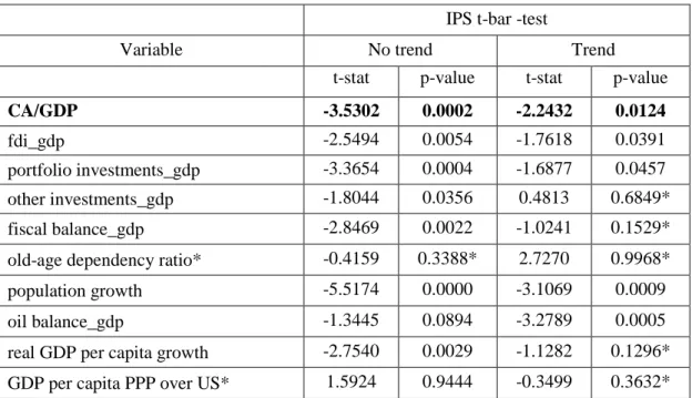
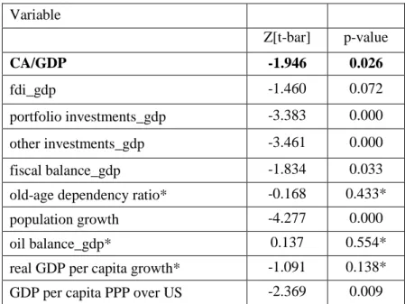
In the MB approach, for the CA estimation, we used mainly a static setup8. The tests confirm the stationarity of our variables, with the exception of the relative old-age dependency ratio9. However, we also found the presence of cross-sectional dependence in our panel (Table 1 and 2). Therefore, we also double-check the stationarity of our variables by using a second generation t-test proposed by Pesaran (2007), which is built for analysis of unit roots in heterogeneous panel setups with cross-section dependence (called CIPS) 10 (Table 3), which confirmed the previous outcome with some exceptions. We found high p-values for the relative old-age dependency ratio, fiscal balance/GDP and real GDP per capita growth. These variables are non-stationary.
[Tables 1, 2 and 3 around here]
We tested for the presence of cointegration by using the Westerlund (2007) error-correction-based panel cointegration test, finding that the variables are not cointegrated11 for the baseline setup (Column 1 in Table 5). We cannot perform such a test with more endogenous variables; therefore we are not able to check the other specifications.
Another test has been provided to test for cointegration in our panel, known as “Pedroni test”12. This is a procedure for heterogeneous panels which allows for more regressors13. In this case, for the baseline and the specification with the NFA position (Column 1 and 2a in Table 5); the null hypothesis of no cointegration is strongly rejected. As reported by Wagner and Hlouskova (2009), “Pedroni test” applying the ADF principle perform best, on the contrary all other tests (Westerlund’s included) have very low power in many circumstances (and virtually none for T ≤ 25, which is our case). The authors conclude that in a situation where the null hypothesis of no cointegration is crucial, the “Pedroni test” is the first choice.
[Table 4 around here]
Given the presence of some non-stationary series and of cointegration in the main setups, the estimations by using the Group Mean (GM)-Fully Modifed OLS (FMOLS) methodology have also been provided. The GM-FMOLS estimator proposed by Pedroni (2000) is indeed an estimator that eliminates this endogeneity bias between dependent variable and regressors and it is less biased in case of static, non-stationary and cointegrated panels even in relatively small samples under a variety of scenarios (Pedroni, 2000). These
8 The IMF also provided the dynamic approach in its article IV. 9
As reported by Medina et al. (2010), the demographic variables may be not-stationary. They argue that these measures seem to be trending during the sample period, but these variables are bounded by construction, and with a longer sample should be stationary (in our case we only have data from 1994 to 2012).
10
Null hypothesis assumes that all series are non-stationary. This t-test is also based on Augmented Dickey-Fuller statistics as IPS (2003) but it is augmented with the cross section averages of lagged levels and first-differences of the individual series (CADF statistics).
11 Robust p-values: Gt=0.53, Ga=0.25, Pt=0.34, Pa=0.36. 12
The test has been conducted by using the RATS command @pancoint. The test is described in Pedroni (1999) and Pedroni (2004).
13
9
estimated coefficients have been used to build the CA norms (see Annex 1, Table 7) as an alternative and extension to our main framework.
In addition, it is worth to recall that we decided not to use a dynamic setup for the calculation of the CA norm14. The dynamic setup has been provided anyway for comparison. This should be done by using the common correlated mean group estimator (CCEMG), which deals with cross-sectional dependence in dynamic panels and allows for heterogeneous coefficients, as explained in Pesaran and Tosetti (2011)15. This structure (also called interactive models or common factor models) introduces in the setup some time-varying unobserved common factors, which represent global factors (crisis or shocks for instance) or spillover effects across the individuals of the panel. The unobserved common factors are proxied by the cross-section averages of the dependent variable and of the regressors. The results for the main specifications are reported in Annex 1 (Table 8).
Ultimately, we decided to keep the structure and the estimation technique as in IMF Article IV estimations, Medina et al. (2010) and Lee et al. (2008) for comparison, in our main analysis. We construct the CA norms starting from these coefficients. We therefore apply the Fixed Effect estimator and the Pooled estimator as in Lee et al. (2008) but correcting the standard error by using the Driscoll-Kraay correction (Hoechle, 2007) for cross-sectional dependence. We also applied the framework as in Medina et al. (2010) estimating the coefficients with Pooled OLS.
The misalignments computed by using the CA norm values coming from the GM-FMOLS coefficients (setup á la Medina et al. (2010)) are also showed as an extension16
. 6. Results
6.1. Expected results
For the Macroeconomic Balance method (and the FEER), we study the fundamentals of the CA. The fiscal balance should be positive, because it brings an increase in savings. Only in the case of full Ricardian equivalence, the private savings fully offset changes in public savings and there is no link. Both the old-age dependency ratio and the population growth are expected to have a negative impact on the CA balance, because both an high number of old people or children should bring a decrease in savings. In this framework, the initial value of NFA is also included. Countries with negative NFA are expected to improve the CA position to preserve long-term solvency, so the sign should be negative (Lane and Milesi-Ferretti, 2004). On the other hand, highly indebted countries typically record negative income flows, which weigh negatively on
14
In our opinion adding a lagged value of the explanatory variable in the study of the determinants of the variable itself to be used to compute the norm, it would be not correct.
15
The CCEMG estimator allows for the empirical setup with cross sectional dependence, time-variant unobservable factors with heterogeneous impact across panel members and fixes problems of identification. This estimator is designed for micro panel models with "large-T, small-N" (Roodman, 2009).
16
10
the CA (Ca’ Zorzi et al., 2012). The sign of the oil balance depends on whether the country is an importer or exporter of oil (importers: declining other imports =positive, see Medina et al. (2010)). The relative income should be positive because as they approach the income level of advanced economies, which means an increase in convergence, CA should improve. We expect to have a negative relative output growth coefficient, which captures relative economic growth with respect to the partners and stronger growth is often linked with a decline in CA because of higher potential, the country can save less today.
We also added a crisis/post crisis dummy (common factor, years from 2008 to 2012) also as a proxy for a structural break. A macroeconomic crisis can decrease the availability of international financing and increase the CA temporarily, therefore we expect a positive sign for the dummy.
Lastly, FDI/GDP17 (Medina et al., 2010 and Rahman, 2008) should be negative. FDIs are more stable investments and less prone to sudden stops. If FDIs are directed to finance the CA deficits, this brings a decline in CA over time, because the method of financing is less uncertain and allows you to borrow and import more.
In addition, in another extension, we use 3 types of flows at the same time: FDIs, which are normally associated with investments in a longer time perspective (it is not always the case in all the CEECs however); portfolio investments and bank loans which should be more related to short-term movements and sudden increase of demand and therefore imports as well. We expect a negative sign for the coefficient for all the types of financing.
6.2. Results for the new EU member states
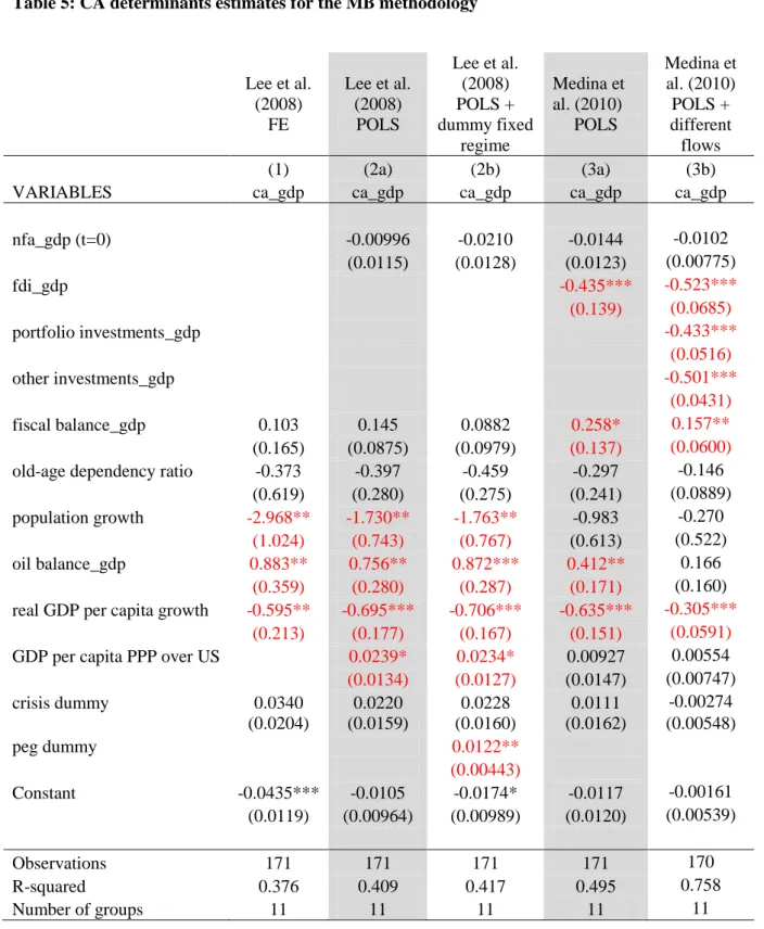
In Table 5, we can see the results of the different specifications in the Columns 1-3. Column (2b) extends the setup by Lee et al. (2008) adding a fixed exchange rate regime dummy, while in Column (3b) (Table 5) we also use other types of foreign capital flows together with the FDIs.
In all the specifications, the coefficients have the correct sign. The only coefficient always significant across the specifications is the relative output growth. Population growth matters if foreign capital flows are not included among the estimators. Oil balance is a key determinant in all the specifications, except when all the types of flows are used. The coefficient of the convergence variable (GDP per capita PPP over US) is, however, much lower (or even not significant in the last two columns) than the growth of real GDP per capita. Therefore, the growth effect is predominant and tends to decrease the CA of these economies, while the convergence component is still not the key factor. The fiscal balance plays an important role in increasing the
17
The investments over GDP (as gross fixed investments) are instead included in the analysis of the fundamentals in Ca’Zorzi et al. (2012). They argue that investment should lead to productivity gains in the future and because of higher expected wealth, it should result in a current account deficit. Moreover, an increase in the domestic demand, brought by the investment, is associated with a worsening of the foreign trade balance. In the case of the CEECs the main source of investments has been, and still is, from abroad. Therefore we decided to include foreign investments in our analysis.
11
CA (or in lowering the deficit) only when flows are added to the framework. Therefore we can see an increase in savings as well when foreign capitals flow into a country. However, the magnitude of the savings is much lower than the one of flows and the negative components prevail.
We also include in an alternative specification a dummy variable for the peggers (1=peg) to control for the exchange rate regimes (Column 2b, Table 5). In this case the coefficient is positive. Therefore the peggers should have a smaller CA deficit in equilibrium with respect to the floaters, which transmits into negative CA gaps (calculated as the equilibrium CA minus the actual CA).
Lastly, in the specifications in Column (3a) and (3b) we included different types of foreign capital flows. In both the cases the FDIs experience a strongly negative and significant coefficient, in line with the expected results. If we add other types of foreign investments (which have been crucial for instance for the Baltic States), their coefficients are negative and significant as well. This effect probably works through an increase in the domestic demand rather than via an increase in wealth expectation due to an increase in productivity. This increase in demand can be indeed brought by the investments, which are associated with a worsening of the trade balance and therefore of the current account.
[Table 5 around here]
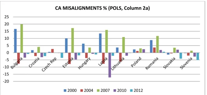
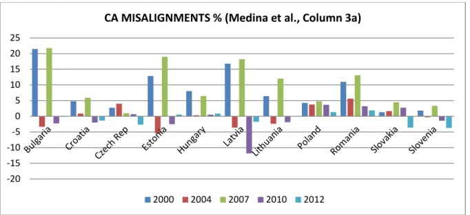
Concerning the misalignments in CA and REER these are very different respect to the ones described by the BEER method (as in Comunale, 2015). The difference in misalignments between Lee’s approach and Medina’s are mainly in magnitude instead. The peak of REER misalignments (2007) follow the behaviour of CA gaps. The “actual”/projected CA is higher than the equilibrium CA and the REER tends to be positively misaligned, i.e. is overvalued. In 2010 and 2012 we can see a rebalancing in the CA, which brings also down the magnitude of the REER misalignments in the recent periods. Therefore, the REERs after the appreciation during boom years are becoming close to the equilibrium values. This conclusion is in line with the previous literature, as for instance in Ajevskis et al. (2012) for the Latvian case. When the Foreign Direct Investments (FDIs) are introduced as a determinant for these countries, the misalignments are larger, in the boom periods (positive misalignments); while in some cases the misalignments are smaller during the crisis (negative misalignments). Therefore, the effect of huge flows of FDIs in some of the CEECs seems to boost the CA in good times and reduce the CA misalignments in bad times. The REERs follow also in this case a similar behaviour.
Looking at the difference in exchange rate regimes, we notice that peggers18 experience generally higher misalignments compared to floaters across the sample. The exception is Romania, whose misalignments in the CA and REER are comparable with the peggers in magnitude, but not in the cyclicality. Croatia here is treated
18
Peggers (or euro area members) are: Bulgaria, Croatia, Estonia, Latvia, Lithuania, Slovakia and Slovenia. Countries with floating regimes are instead: Czech Republic, Hungary, Poland and Romania.
12
as an “acceding” country, because our data are until 2012. The Croatian misalignments are not as big as the ones of other peggers.
[Figures 3 and 4 around here]
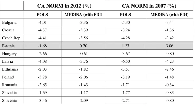
If we look at the CA equilibrium values, i.e. norms, in the most recent year available, the higher deficits (above 4%) are in Bulgaria, Croatia, Czech Republic and Latvia. The only country that should have a CA surplus as equilibrium value is Estonia (0.7%) when FDIs are taken into account. In any case, when FDIs are included, the CA norms are smaller in magnitude. This difference is extremely wide in Hungary and Estonia. If we calculate the CA norm in 2007 instead, Estonia experienced again a positive CA norm, while Latvia, Bulgaria and Czech Republic very negative CA norms. Therefore the capital do not always flow downstream in the case of CEECs, i.e. where there is higher capital needs and an increase in imports bring higher current account deficit.
[Table 6 around here]
Lastly, we focus on the situation in the Baltics, as an interesting case study in the area. The cyclicality in both CA and REER misalignments is clear in this case. Latvia experienced the largest swing in both the misalignments, while the differences in the Lithuanian case were smaller. This has been probably caused by the fact that Latvia showed the highest deficit in the CA among the Baltic States in 2007: 22% of GDP; while in Lithuania was of 14% of GDP and in Estonia of 16% of GDP. Moreover, Latvia was the only Baltic country to request in September 2008 the EU-IMF funding assistance (Sufficiently large support package: €7.5 billion, incl. €3.1bn European Commission, €1.7bn IMF, €1.8bn Nordics). This can have influenced the CA and REER giving a largest drop in the misalignments in 2010, because in the calculation of CA norm the external bailout funding is not included and the actual CA in 2010 was therefore much lower than the norm. The REER followed again the CA behaviour and was negatively misaligned by more than 26% (if FDIs included). This real undervaluation, which means an increase in country’s competitiveness, might also have helped Latvia in recovering via an increasing in the exports and then the trade balance19. In 2012 Latvia had still showed a negative misalignments but by only 2-4%. In 2012 we can see a tendency towards the equilibrium in CA and REER is all the countries indeed. Estonia has a positive misalignment again in the CA and REER (around 1%).
[Figures 5a and 5b around here]
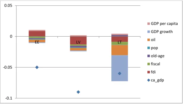
We calculated therefore the contribution of each factors in determining the CA in the Baltic States in the period 2004-2007 and 2008-2012, by using the coefficients from the setup with FDIs (Column (3a), Table 5).
19
The recovery in the CA can be explained as a joint work of increase competitiveness (here as declining in REER) and a cyclical component in the financial variables (see Comunale and Hessel, 2014).
13
The FDI component is crucial for Estonia, in order to have a lower CA deficit growth rate in the boom period, while FDIs contribute on a negative way to the rate in Lithuania and Latvia. The real GDP per capita growth relative to the partners is instead key for Lithuania. This means that the stronger growth after the EU accession brought in Lithuania a sizeable decline in savings and an increase in demand and imports. The growth component has been important instead for Estonia and Latvia in the post-crisis period, limiting the rebalancing in the CA. The internal devaluation, mainly via a huge decrease in public spending and salaries, helped all the Baltic States in their way towards the equilibrium. Indeed the fiscal balance plays a key role especially in Latvia. In Lithuania the rebalancing in the CA was more a joint results of changing in fiscal policy, increasing in more productive FDIs and aging/population factors.
[Figure 6 and 7 around here] 7. Extensions: cointegrated static setup and dynamic setup
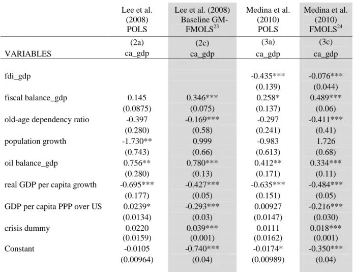
In the Annex 1, the estimations by using the GM-FMOLS are also provided (Table 7) as an extension of our baseline framework. The fiscal balance has the correct sign and it is strongly significant, as it is for old-age dependency ratio, growth real GDP per capita and oil balance. The dummy variable for the crisis has the correct sign as well and becomes significant. The sign of FDIs is still negative but the magnitude is much smaller with respect to the setup estimated by pooled OLS. On the other hand, the population growth shows a positive coefficient, even if not significant, which is not what we expected. The sign of GDP per capita in PPP over the US data, i.e. the relative income, is strongly negative and significant.
[Table 7 around here]
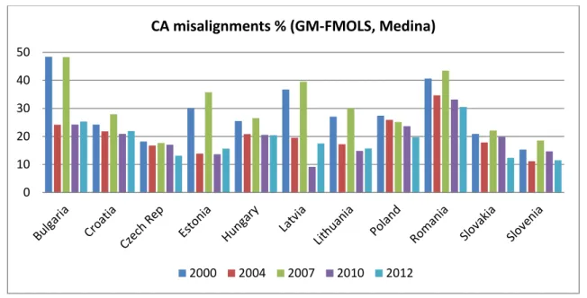
The misalignments computed by using the CA norm values coming from these GM-FMOLS coefficients (setup á la Medina et al. (2010), Table 7 Column (3c)) are also showed here as an extension20
. The misalignments for the CA and REER are definitely wider than in our baseline framework. The cyclicality in the misalignments is reduced. Moreover, with this approach, there is an increasing in the misalignments after 2010 in some member states like the Baltics, Bulgaria and Croatia. This can be considered as a “recovery” period for these countries and the CA deficit may be already starting widening because of an increase in the domestic demand (and relative imports) and FDI flows. The REER misalignments again, seem to follow the behaviour of the CA, even if in this case the cyclicality is more evident. The higher misalignments in the boom period can be seen in Bulgaria, the Baltics (especially Latvia), Poland and Romania. In 2012 they are still very high in Poland and Romania.
[Figure 8 around here]
20
14
Lastly, we estimate the dynamic setups by using the common correlated mean group estimator (CCEMG), which deals with cross-sectional dependence in dynamic panels and allows for heterogeneous coefficients, as explained in Pesaran and Tosetti (2011). We do this exercise for the specifications from Lee et al. (2008) formerly estimated with fixed effects and pooled OLS (Column 1 and 2a, Table 5) and from Medina et al. (2010) with FDIs (Column 3a, Table 5). The results are presented in Table 8.
[Table 8 around here]
In these results the unobserved common factors are proxied by the cross-section averages of the dependent variable and of the regressors. The main variable, which seems to determine the CA, is the oil balance, as in the static setup; however these unobserved factors play an important role. In the more complete framework, borrowed from Medina et al. (2010), factors related to oil balance, the CA itself and real GDP per capita growth are significant as well. The sign for the unobserved oil balance factor and real GDP per capita growth are the opposite as expected (Table 8, Column (3)). Therefore, while a decrease in imports values or/and quantities can have had a positive effect on the CA, some global factors like shocks in oil prices or supply might have played a role in the opposite direction, worsening, after all, the CA balance of the CEECs. The relative GDP per capita growth is not significant in our specifications here, but the coefficient for the related unobserved factor is stead positive and significant, which can imply a role for spillovers among the members. An increase in the GDP per capita of partners can affect positively the CA via a rise in foreign demand which leads to a more exports and a better trade balance for the country.
8. Conclusions and policy implications
Following the standard IMF CGER methodology (see Lee et al. 2008) for the estimation of real effective exchange rate (REER) misalignments, we conduct an assessment of the current account position and competitiveness of the Central Eastern EU new member states (CEECs). We analyse these issues by using a panel setup of 11 EU new member states over the period 1994-2012 in static and dynamic frameworks, also controlling for the presence of cross-sectional dependence, checking specifically for the role of exchange rate regimes, capital flows and global factors.
The estimated coefficients are in line with the expectations. Moreover the foreign capital flows, the oil balance and relative output growth seem to play a crucial role in explaining the current accounts. In addition, some global factors like shocks in oil prices or supply might have played a role in the opposite direction, worsening the CA balance of the CEECs. Having a pegged exchange rate regime (or being part of the euro zone) affects positively the current account, but the resulted misalignments are bigger. The REERs behave in line with the current account gaps, which experience a clear cyclical behaviour. We find a high overvaluation in 2007 for Bulgaria, the Baltics and Romania (in line with Rahman, 2008), followed by a rebalancing from 2010 onwards. The CAs and REERs are getting close to equilibria in 2012 in most of the countries. The
15
rebalancing is completed for some countries less misaligned in the past like Poland and Czech Republic, but also in the case of Lithuania. When the Foreign Direct Investments (FDIs) are introduced as a determinant for these countries, the misalignments are larger, in the boom periods (positive misalignments); while the misalignments are smaller during the crisis (negative misalignments). Therefore, the effect of huge flows of FDIs in some of the CEECs seems to boost the CA in good times and reduce the CA misalignments in bad times. The REERs follow also in this case a similar behaviour.
The main policy implication involves the future behaviour (in terms of an increase of REERs or a decrease in CA deficit norms). Are further actions to rebalance the CAs needed? Should we look at a balanced CA (as close to zero as possible) or at the CA norm, which can be different from zero and can change over time, as shown in the paper.
Are the REER and its components the right instruments (the role of the financial cycle may be as important21)? We are indeed working on an analysis applying a closer interaction between the misalignments in the REER, the CA and financial gaps.
21
16 TABLES AND FIGURES
Figure 1: REERs in the new EU member states
Figure 2: CA over GDP in the new EU member states 40 50 60 70 80 90 100 110 120 130 140 19 94 19 95 19 96 19 97 19 98 19 99 20 00 20 01 20 02 20 03 20 04 20 05 20 06 20 07 20 08 20 09 20 10 20 11 20 12 R EE R d e fl ate d b y C PI 2005= 100
REERs in the new EU member states
Bulgaria Croatia Czech Rep. Estonia Hungary Latvia Lithuania Poland Romania Slovakia Slovenia -30 -25 -20 -15 -10 -5 0 5 10 15 19 94 19 95 19 96 19 97 19 98 19 99 20 00 20 01 20 02 20 03 20 04 20 05 20 06 20 07 20 08 20 09 20 10 20 11 20 12 CA i n % G D P
CA/GDP in the new EU member states
Bulgaria Croatia Czech Republic Estonia Hungary Latvia Lithuania Poland Romania Slovak Republic Slovenia
17
Table 1: Stationarity test: Im-Pesaran-Shin (IPS) panel unit root test IPS t-bar -test
Variable No trend Trend
t-stat p-value t-stat p-value
CA/GDP -3.5302 0.0002 -2.2432 0.0124
fdi_gdp -2.5494 0.0054 -1.7618 0.0391
portfolio investments_gdp -3.3654 0.0004 -1.6877 0.0457 other investments_gdp -1.8044 0.0356 0.4813 0.6849* fiscal balance_gdp -2.8469 0.0022 -1.0241 0.1529* old-age dependency ratio* -0.4159 0.3388* 2.7270 0.9968* population growth -5.5174 0.0000 -3.1069 0.0009 oil balance_gdp -1.3445 0.0894 -3.2789 0.0005 real GDP per capita growth -2.7540 0.0029 -1.1282 0.1296* GDP per capita PPP over US* 1.5924 0.9444 -0.3499 0.3632*
Note: In the IPS-test, one lag has been imposed. IPS can be used in case of unbalanced panel, but requires that there are no gaps in each individual time series. Other tests require that the panels are strongly balanced. The variable in bold font is the dependent variable in our equation. Null hypothesis assumes that all series are non-stationary.
* means non-stationarity for all series.
Table 2: Cross-sectional independence test (Pesaran’s test)
Test Probability Equation in Table 5 Column (1) 6.182 0.0000 Column (2a) 6.620 0.0000 Column (2b) 6.476 0.0000 Column (3a) 6.534 0.0000 Column (3b) 2.596 0.0094
Note: Pesaran’s test for cross-sectional dependence following the methods shown in Pesaran (2004). Pesaran's statistic follows a standard normal distribution and it is able to handle balanced and unbalanced panels. It tests the hypothesis of cross-sectional independence in panel data models.
18
Table 3: Stationarity test: second generation t-test by Pesaran (2007) for unit roots in heterogeneous panels with cross-section dependence (CIPS)
Variable Z[t-bar] p-value CA/GDP -1.946 0.026 fdi_gdp -1.460 0.072 portfolio investments_gdp -3.383 0.000 other investments_gdp -3.461 0.000 fiscal balance_gdp -1.834 0.033
old-age dependency ratio* -0.168 0.433*
population growth -4.277 0.000
oil balance_gdp* 0.137 0.554*
real GDP per capita growth* -1.091 0.138* GDP per capita PPP over US -2.369 0.009
Note: Null hypothesis assumes that all series are non-stationary. 1 lag has been imposed. This t-test is also based on Augmented Dickey-Fuller statistics as IPS (2003) but it is augmented with the cross section averages of lagged levels and first-differences of the individual series (CADF statistics)22. *means non-stationarity for all series.
Table 4: Pedroni test for cointegration
Panel group RHO-stat Equation in Table 5
Column (1) 4.02*
Column (2a) – no crisis dummy 4.56*
Column (2b) (more than 8 endogenous variables) Column (3a) (more than 8 endogenous variables) Column (3b) (more than 8 endogenous variables)
Note: This is a revised procedure for cointegration tests in heterogeneous panels with multiple regressors ("Pedroni tests"). We applied 1 lag (no trend). All reported values are distributed N (0,1) under null of no cointegration. In case of very small panel (as it is here) in Pedroni (2004) is explained that group stat is better because less distortive and more conservative. If group RHO-stat Panel = -2.336 then p-value = 0.010 (Source: Maeso-Fernandez et al., 2004) with N=25. In my case N = 11, we can apply 2-tails t-stat (Rho-stat is distributed approximately as Student's t distribution with n − 2 degrees of freedom under the null hypothesis): 10% with rejection of the null if it is higher than 1.860; 5% rejection if higher than 2.306; 1% rejection if higher than 3.355.
*means cointegration.
22
The command in Stata is called -pescadf- and it has been built by Piotr Lewandowski, Warsaw School of Economics, Institute for Structural Research.
19
Table 5: CA determinants estimates for the MB methodology
Lee et al. (2008) FE Lee et al. (2008) POLS Lee et al. (2008) POLS + dummy fixed regime Medina et al. (2010) POLS Medina et al. (2010) POLS + different flows (1) (2a) (2b) (3a) (3b)
VARIABLES ca_gdp ca_gdp ca_gdp ca_gdp ca_gdp
nfa_gdp (t=0) -0.00996 -0.0210 -0.0144 -0.0102 (0.0115) (0.0128) (0.0123) (0.00775) fdi_gdp -0.435*** -0.523*** (0.139) (0.0685) portfolio investments_gdp -0.433*** (0.0516) other investments_gdp -0.501*** (0.0431) fiscal balance_gdp 0.103 0.145 0.0882 0.258* 0.157** (0.165) (0.0875) (0.0979) (0.137) (0.0600)
old-age dependency ratio -0.373 -0.397 -0.459 -0.297 -0.146
(0.619) (0.280) (0.275) (0.241) (0.0889)
population growth -2.968** -1.730** -1.763** -0.983 -0.270
(1.024) (0.743) (0.767) (0.613) (0.522)
oil balance_gdp 0.883** 0.756** 0.872*** 0.412** 0.166
(0.359) (0.280) (0.287) (0.171) (0.160)
real GDP per capita growth -0.595** -0.695*** -0.706*** -0.635*** -0.305***
(0.213) (0.177) (0.167) (0.151) (0.0591)
GDP per capita PPP over US 0.0239* 0.0234* 0.00927 0.00554
(0.0134) (0.0127) (0.0147) (0.00747) crisis dummy 0.0340 0.0220 0.0228 0.0111 -0.00274 (0.0204) (0.0159) (0.0160) (0.0162) (0.00548) peg dummy 0.0122** (0.00443) Constant -0.0435*** -0.0105 -0.0174* -0.0117 -0.00161 (0.0119) (0.00964) (0.00989) (0.0120) (0.00539) Observations 171 171 171 171 170 R-squared 0.376 0.409 0.417 0.495 0.758 Number of groups 11 11 11 11 11
Note: Standard errors in parentheses (Driscoll-Kraay correction for CSD) *** p<0.01, ** p<0.05, * p<0.1. Other investments are mainly bank loans. The crisis dummy is equal to 1 in the period 2008-2012. The peg dummy is equal to 1 in case of a de facto fixed regime (or if the country is in the euro zone) in a certain year. Column (2b) and (3b) are alternative specifications/extensions of the setups in (2a) and (3a).
20
Figure 3: CA and REER misalignments by using the MB methodology (POLS from Lee et al, 2008) -20 -15 -10 -5 0 5 10 15 20 25
CA MISALIGNMENTS % (POLS, Column 2a)
2000 2004 2007 2010 2012 -40 -30 -20 -10 0 10 20 30 40 50
REER MISALIGNMENTS % (POLS, Column 2a)
21
Figure 4: CA and REER misalignments by using the MB methodology (Medina et al, 2010: FDI/GDP is included in the regressors)
-20 -15 -10 -5 0 5 10 15 20 25
CA MISALIGNMENTS % (Medina et al., Column 3a)
2000 2004 2007 2010 2012 -40 -30 -20 -10 0 10 20 30 40 50
REER MISALIGNMENTS % (Medina et al., Column 3a)
22 Figure 5a: CA misalignments in the Baltic States
2000 2004 2007 2010 2012
POLS 10.07 -7.87 17.21 -4.75 -1.82
MEDINA (with FDI) 21.82 -9.24 32.31 -4.27 0.95
-15.00 -10.00 -5.00 0.00 5.00 10.00 15.00 20.00 25.00 30.00 35.00
Estonia: % CA misalignments
2000 2004 2007 2010 2012 POLS 13.47 -7.71 15.94 -17.25 -2.11MEDINA (with FDI) 16.81 -3.61 18.22 -11.87 -1.79
-20.00 -15.00 -10.00 -5.00 0.00 5.00 10.00 15.00 20.00
Latvia: % CA misalignments
2000 2004 2007 2010 2012 POLS 3.65 -6.14 10.97 -2.08 -0.22MEDINA (with FDI) 6.43 -2.40 12.02 -1.87 0.00
-8.00 -6.00 -4.00 -2.00 0.00 2.00 4.00 6.00 8.00 10.00 12.00 14.00
Lithuania: % CA misalignments
23 Figure 5b: REER misalignments in the Baltic States
2000 2004 2007 2010 2012
POLS 17.11 -13.37 29.25 -8.07 -3.09
MEDINA (with FDI) 21.82 -9.24 32.31 -4.27 0.95
-20.00 -10.00 0.00 10.00 20.00 30.00 40.00
Estonia: % REER misalignments
2000 2004 2007 2010 2012
POLS 30.36 -17.37 35.91 -38.88 -4.76
MEDINA (with FDI) 37.86 -8.13 41.04 -26.75 -4.02
-50.00 -40.00 -30.00 -20.00 -10.00 0.00 10.00 20.00 30.00 40.00 50.00
Latvia: % REER misalignments
2000 2004 2007 2010 2012
POLS 7.62 -12.81 22.87 -4.33 -0.45
MEDINA (with FDI) 13.40 -5.00 25.06 -3.90 0.00
-15.00 -10.00 -5.00 0.00 5.00 10.00 15.00 20.00 25.00 30.00
24
Table 6: CA norm (i.e. equilibrium value) in 2012 and 2007
CA NORM in 2012 (%)
CA NORM in 2007 (%)
POLS MEDINA (with FDI) POLS MEDINA (with FDI)
Bulgaria -4.01 -3.36 -5.30 -3.44 Croatia -4.37 -3.39 -3.24 -1.36 Czech Rep -4.41 -3.56 -4.28 -3.42 Estonia -1.68 0.70 1.27 3.06 Hungary -2.66 -0.61 -3.67 -0.80 Latvia -4.08 -3.76 -6.50 -4.23 Lithuania -2.03 -1.82 -3.51 -2.46 Poland -3.28 -2.06 -3.19 -1.48 Romania -2.65 -1.43 -1.71 -0.34 Slovakia -1.69 -1.17 -1.77 -0.83 Slovenia -3.46 -2.09 -2.71 -0.80
Note: We calculate the CA norm as the coefficients from the determinants multiplied by the projected variables from IMF WEO or UNDESA (for year 2012 the latest projections are for 2019). In this calculation the dummies are not included.
25
Figure 6: Factor analysis for the Baltic States 2004-2007, by using Medina et al. (2010) setup
Note: These are the coefficients of the determinants multiplied by the difference in the value of the variables. Ca_gdp is the difference of CA over GDP in the period (2004-2007). On the y-axis: the difference in the CA over GDP in the period (2004-2007) are expressed as a percentage, 0.05 is equal to 5%.
Figure 7: Factor analysis for the Baltic States 2008-2012, by using Medina et al. (2010) setup
Note: These are the coefficients of the determinants multiplied by the difference in the value of the variables. Ca_gdp is the difference of CA over GDP in the period (2008-2012). On the y-axis: the difference in the CA over GDP in the period (2008-2012) are expressed as a percentage, 0.05 is equal to 5%. -0.1 -0.05 0 0.05 EE LV LT GDP per capita GDP growth oil pop old-age fiscal fdi ca_gdp -0.1 -0.05 0 0.05 0.1 0.15 EE LV LT GDP per capita GDP growth oil pop old-age fiscal fdi ca_gdp
26 ANNEX 1
Table 7: GM-FMOLS estimations of CA determinants
Lee et al. (2008) POLS Lee et al. (2008) Baseline GM-FMOLS23 Medina et al. (2010) POLS Medina et al. (2010) FMOLS24 (2a) (2c) (3a) (3c)
VARIABLES ca_gdp ca_gdp ca_gdp ca_gdp
fdi_gdp -0.435*** -0.076***
(0.139) (0.044)
fiscal balance_gdp 0.145 0.346*** 0.258* 0.489***
(0.0875) (0.075) (0.137) (0.06)
old-age dependency ratio -0.397 -0.169*** -0.297 -0.411***
(0.280) (0.58) (0.241) (0.41)
population growth -1.730** 0.999 -0.983 1.726
(0.743) (0.66) (0.613) (0.68)
oil balance_gdp 0.756** 0.780*** 0.412** 0.334***
(0.280) (0.13) (0.171) (0.11)
real GDP per capita growth -0.695*** -0.427*** -0.635*** -0.484***
(0.177) (0.05) (0.151) (0.05)
GDP per capita PPP over US 0.0239* -0.293*** 0.00927 -0.216***
(0.0134) (0.03) (0.0147) (0.030) crisis dummy 0.0220 0.039*** 0.0111 0.018*** (0.0159) (0.001) (0.0162) (0.001) Constant -0.0105 -0.740*** -0.0174* -0.350*** (0.00964) (0.04) (0.00989) (0.04)
Note: Standard errors are in parentheses: *** p<0.01, ** p<0.05, * p<0.1. In Column (2a) and (3a) are reported the results by using POLS with correction for cross-sectional dependence as in Lee et al. (2008) and the setup from Medina et al. (2010) as in Table 5. In Column (2c) and (3c) are reported the GM-FMOLS estimations taken with 1 lag for the regressors and calculated by the command @panelfm in RATS.
23
Here nfa_gdp (t=0) is not included, because in that case @panelfm cannot be used (it created a non-invertible matrix). 24
27
Figure 8: CA and REER misalignments by using the MB methodology (GM-FMOLS for the model á la Medina et al. (2010))
0 10 20 30 40 50
CA misalignments % (GM-FMOLS, Medina)
2000 2004 2007 2010 2012 0 20 40 60 80 100 120 140
REER misalignments % (GM-FMOLS, Medina)
28
Table 8: Common Correlated Mean Group (CCEMG) estimations of CA determinants
Lee et al. (2008) Baseline (former FE)
CCEMG Lee et al. (2008) (former POLS) CCEMG Medina et al. (2010) (former POLS) CCEMG (1) (2) (3)
VARIABLES ca_gdp ca_gdp ca_gdp
L1.ca_gdp 0.0847 0.482 0.107 (0.321) (0.321) (0.309) fdi_gdp -0.158 (0.151) fiscal balance_gdp -0.285 0.623 0.170 (0.417) (0.557) (0.197)
old-age dependency ratio -1.083 -2.455 -0.703
(0.738) (1.779) (0.791)
population growth 1.227 6.485* 1.034
(2.237) (3.567) (1.178)
oil balance_gdp 1.329 2.035* 1.355***
(0.815) (1.061) (0.407)
real GDP per capita growth -0.0870 -0.137 -0.620
(0.514) (0.621) (0.409)
GDP per capita PPP over US -0.157 0.0889
(0.210) (0.145)
crisis dummy 0.0077 -0.00795 -0.0180
(0.0307) (0.0309) (0.0290)
Constant -0.0598 0.0349 -0.00511
(0.0900) (0.298) (0.145)
Significant unobserved factors
Related to ca_gdp 0.712* 0.879*** 0.786**
(0.412) (0.276) (0.313)
Related to population growth 6.77** (2.860)
Related to oil balance_gdp -1.987*
(1.074)
Related to real GDP per capita growth 0.909**
(0.501)
Note: Standard errors are in parentheses: *** p<0.01, ** p<0.05, * p<0.1. Here are reported the CCEMG estimations (Stata command –xtmg- by Markus Eberhardt).
29 ANNEX 2: DATA DESCRIPTION AND SOURCES
Countries Bulgaria, Croatia, Czech Republic, Estonia, Hungary, Latvia, Lithuania,
Poland, Romania, Slovakia and Slovenia
Variable Sources Description
reer Eurostat REER 2005=100. Deflator: CPI ; vis-à-vis 37 partner countries ca_gdp IMF WEO CA in million USD / over GDP in current USD
nfa_gdp (t0) Updated EWN (Lane and MF, 2007)
nfa_gdp in 1993, otherwise the first year available (Croatia 1996)
fdi_gdp IMF WEO (net
inflows)
Foreign Direct Investments in current USD. Inflows. Over GDP in current USD. From Medina et al., 2010
portfolio
investments_gdp
IMF WEO (net inflows)
Portfolio Investments in current USD. Inflows. Over GDP in current USD.
other
investments_gdp
IMF WEO (net inflows)
Other Investments (mainly bank loans) in current USD. Inflows. Over GDP in current USD.
fiscal balance_gdp IMF WEO General government revenue minus expenditure over GDP (relative to partners)
old-age
dependency ratio
WB WDI population > 65y/population between 15-65 (relative to partners) - from Chinn & Prasad, 2003 or Medina et al., 2010 population growth WB WDI Population growth (annual %) (relative to partners)
oil balance_gdp IMF WEO25 Ratio of Oil Balance to nominal GDP in current USD real GDP per capita
growth
UNCTAD Real GDP growth rates per capita, (relative to partners)
GDP per capita PPP over US
IMF WEO Log of GDP per capita, PPP (constant 2005 international $) over GDP per capita, PPP of US
crisis dummy dummy from 2008 to 2012 =1
peg dummy dummy Countries with a pegged exchange rate regime or in the euro area = 1
Note: Projections: from WEO IMF and UN DESA for demographics; Growth rates: avg of 5 years (2014/2019 for real GDP per capita growth or 2015/2020 for population growth)
25Starting with the October 2013 WEO, the Value of oil imports (TMGO) and Value of oil exports (TXGO) countries’ data are no longer be available in the external WEO Database.
30 REFERENCES
Ajevskis V.,Rimgailaite R., Rutkaste U. and Tkacevs O. (2012). The Assesment of Equilibrium Real Exchange Rate of Latvia. Working Papers 2012/04, Latvijas Banka.
Ajevskis V.,Rimgailaite R., Rutkaste U. and Tkacevs O. (2015) The equilibrium real exchange rate: pros and cons of different approaches with application to Latvia. Baltic Journal of Economics, 14:1-2, 101-123.
Alberola, E., Cervero, S.G., Lopez, H. &Ubide, A. (1999).Global equilibrium exchange rates: Euro, Dollar, ‘ins’, ‘outs’ and other major currencies in a panel cointegration framework. IMF Working Paper WP/99/175, International Monetary Fund.
Alberola, E., Garcia-Cervero, S., Lopez, H., &Ubide, A. (2002). Quo vadis euro?.European Journal of Finance, 8(4), 352-370.
Alberola, E. (2003). Misalignment, liabilities dollarization and exchange rate adjustment in Latin America. Banco de España documento de trabajon°0309, Banco de España, Madrid.
Athukorala, P. C., & Rajapatirana, S. (2003). Capital inflows and the real exchange rate: a comparative study of Asia and Latin America. The World Economy, 26(4), 613-637.
Babecký J., Bulíř A. and Šmídková K. (2010). Sustainable Real Exchange Rates in the New EU Member States; What Did the Great Recession Change. IMF Working Papers 10/198, International Monetary Fund.
Bems, R., & de Carvalho Filho, I. (2009). Current account and precautionary savings for exporters of exhaustible resources. IMF Working Paper WP/09/33, International Monetary Fund.
Bénassy-Quéré, A., Béreau, S. & Mignon, V. (2010).On the complementarity of equilibrium exchange-rate approaches.Review of International Economics, 18(4), 618-632.
Blackburne III, E. F., & Frank, M. W. (2007).Estimation of nonstationary heterogeneous panels. Stata Journal, 7(2), 197-208.
Bussière, M., Fratzscher, M., Müller, G. (2006). Current account dynamics in OECD and new EU member states: an intertemporal approach. Journal of Economic Integration 21 (3), 593-618.
Bussière M., Ca' Zorzi M., Chudik A. and Dieppe A. (2010) ‘Methodological advances in the assessment of equilibrium exchange rates’, ECB Working Paper Series 1151.
Calderon, C. A, Chong A. and Loayza, N.V. (2002). Determinants of Current Account Deficits in Developing Countries. Contributions to Macroeconomics, 2 (1), Article 2.
Carrera, J. E., & Restout, R. (2008).Long Run Determinants of Real Exchange Rates in Latin America.No. 0811. Groupe d'Analyseet de Théorie Economique (GATE), Centre national de la recherche scientifique (CNRS), Université Lyon 2, Ecole Normale Supérieure.
Ca’Zorzi, M., Chudik, A., & Dieppe, A. (2012). Thousands of models, one story: Current account imbalances in the global economy. Journal of International Money and Finance, 31(6), 1319-1338. Chinn, M. D., & Prasad, E. S. (2003). Medium-term determinants of current accounts in industrial and developing countries: an empirical exploration. Journal of International Economics, 59(1), 47-76.
31
Chudik, A., & Mongardini, J. (2007). In search of equilibrium: estimating equilibrium real exchange rates in Sub-Saharan African countries. IMF Working Papers WP/07/90, International Monetary Fund.
Clark, P. B., & MacDonald, R. (1999).Exchange Rates and Economic Fundamentals: a Methodological Comparison of BEERS and FEERS. IinEquilibrium Real Exchange Rates, ed. by R. MacDonald and J.L. Stein (Massachusetts: Kluwer Academic Publishers), pp. 209-40.
Combes, J. L., Kinda, T., & Plane, P. (2012). Capital flows, exchange rate flexibility, and the real exchange rate. Journal of Macroeconomics, 34(4), 1034-1043.
Comunale, M. & Hessel, J. (2014).Current Account Imbalances in the Euro Area: Competitiveness or Financial Cycle? DNB Working paper n.443.
Comunale, M. (2015). Long-Run Determinants and Misalignments of the Real Effective Exchange Rate in the EU. Bank of Lithuania, Working Paper Series No. 18/2015.
Corden, W. M. (1994). Economic Policy, Exchange Rates, and the International System. University of Chicago Press.
Crespo-Cuaresma, J., Fidrmuc, J., & Antoinette, M. (2004).Exchange Rate Developments and Fundamentals in Four EU Accession and Candidate Countries: Bulgaria, Croatia, Romania and Turkey. Focus on European Economic Integration, Oesterreichische Nationalbank, 2, 04.
Edwards, S. (1989). Real Exchange Rates, Devaluation and Adjustment: Exchange Rate Policy in Developing Countries. Cambridge, Massachusetts: MIT Press.
Égert, B., & Lahrèche-Révil, A. (2003).Estimating the fundamental equilibrium exchange rate of Central and Eastern European countries: The EMU enlargement perspective. (No. 2003-05). CEPII. Égert, B., & Lommatzsch, K. (2005). Equilibrium exchange rates in the transition: The tradable price-basedreal appreciation and estimation uncertainty (pp. 205-239). Springer Berlin Heidelberg.
Égert, B., & Halpern, L. (2006). Equilibrium exchange rates in Central and Eastern Europe: A meta-regression analysis. Journal of banking & Finance, 30(5), 1359-1374.
Halpern, L., & Wyplosz, C. (1997).Equilibrium exchange rates in transition economies. Staff Papers-International Monetary Fund, 430-461.
Hoechle, D. (2007). Robust standard errors for panel regressions with cross-sectional dependence. Stata Journal, 7(3), 281.
Im, K. S., Pesaran, M. H., & Shin, Y. (2003).Testing for unit roots in heterogeneous panels.Journal of econometrics, 115(1), 53-74.
Isard, P., & Faruqee, H. (1998). Exchange rate assessment: Extension of the macroeconomic balance approach. IMF Occasional paper 167. International Monetary Fund.
Jaumotte, F., & Sodsriwiboon P. (2010). Current Account Imbalances in the Southern Euro Area. IMF Working Papers WP/10/139, International Monetary Fund.
Jeong, S. E., Mazier, J., & Saadaoui, J. (2010). Exchange rate misalignments at world and European levels: a FEER approach. International Economics, 121, 25-57.
32
Lane, P. R., & Milesi-Ferretti, G. M. (2002).External wealth, the trade balance, and the real exchange rate. European Economic Review, 46(6), 1049-1071.
Lane, P. R., & Milesi-Ferretti, G. M. (2004).The transfer problem revisited: Net foreign assets and real exchange rates. Review of Economics and Statistics,86(4), 841-857.
Lane, P. R., & Milesi-Ferretti, G. M. (2007).The external wealth of nations mark II: Revised and extended estimates of foreign assets and liabilities, 1970–2004.Journal of international Economics, 73(2), 223-250.
Lane, P. R., & Shambaugh, J. C. (2010). Financial exchange rates and international currency exposures. The American Economic Review, 518-540.
Lee, J., Ostry, J. D., Milesi-Ferretti, G. M., Ricci, L. A., & Prati, A. (2008).Exchange rate assessments: CGER methodologies. IMF Occasional Papers 261, International Monetary Fund. Lòpez-Villavicencio, A., Mazier, J., & Saadaoui, J. (2012). Temporal dimension and equilibrium exchange rate: A FEER/BEER comparison. Emerging Markets Review, 13(1), 58-77.
MacDonald, R. (2000). Concepts to calculate equilibrium exchange rates: an overview. No. 2000, 03. Discussion paper Series 1/Volkswirtschaftliches Forschungszentrum der Deutschen Bundesbank. MacDonald, R. (2007). Exchange Rate Economics: Theories and Evidence (Second Edition of Floating Exchange Rates: Theories and Evidence), Routledge, 2007.
MacDonald, R., & Dias, P. (2007). Behavioural equilibrium exchange rate estimates and implied exchange rate adjustments for ten countries. Peterson Institute of International Economics, February. Maeso–Fernandez, F., Osbat, C., & Schnatz, B. (2002). Determinants of the euro real effective exchange rate: A BEER/PEER approach. Australian Economic Papers, 41(4), 437-461.
Maeso-Fernandez, F., Osbat, C., & Schnatz, B. (2004). Towards the estimation of equilibrium exchange rates for CEE acceding countries: methodological issues and a panel cointegration perspective. ECB Working Paper Series 353. European Central Bank.
Maeso-Fernandez, F., Osbat, C., & Schnatz, B. (2005). Pitfalls in estimating equilibrium exchange rates for transition economies. Economic Systems, 29(2), 130-143.
Medina, L., Prat, J., & Thomas, A. H. (2010). Current Account Balance Estimates for Emerging Market Economies. IMF Working Paper WP/10/43, International Monetary Fund.
Nabil A., Jeong S.E., Mazier J., Saadaoui J. Exchange Rate Misalignments and International Imbalances a FEER Approach for Emerging Countries. Economie internationale 4/2010 (n° 124) , p. 31-74
Obstfeld M. (2012). Does the Current Account Still Matter? American Economic Review, American Economic Association, vol. 102(3), pages 1-23, May.
Pesaran, M. H., (2004) General Diagnostic Tests for Cross Section Dependence in Panels. CESifo Working Paper Series No. 1229; IZA Discussion Paper No. 1240.
Pesaran M.H., Tosetti E. (2011) Large panels with common factors and spatial correlation. Journal of Econometrics 161 (2011) 182—202.