Lecture Notes on Info-gaps in Project Management Knowledge Areas

(1)

Info-gaps in Project Management Knowledge Areas

Yakov Ben-Haim

Yitzhak Moda’i Chair in Technology and Economics Faculty of Mechanical Engineering Technion — Israel Institute of Technology

Haifa 32000 Israel

http://www.technion.ac.il/yakov [email protected] Source material:

•Project Management Institute,A Guide to the Project Management Body of Knowledge, (PMBOK Guide), 2000.

• Kerzner, Harold, Project Management: A Systems Approach to Planning, Scheduling, and Con-trolling, 7th ed., John Wiley, 2001.

A Note to the Student: These lecture notes are not a substitute for the thorough study of books. These notes are no more than an aid in following the lectures.

1 Project Integration Management

¶ Project integration management: the PMI perspective1: •Coordinate elements of the project.

•Identify and make trade-oﬀs between competing objectives. •Major processes for integration:

◦ Develop consistent, coherent project plan document. ◦ Carry out the project plan.

◦ Coordinate changes in the plan.

¶ Centraltrade-oﬀs which we will study:

•Robustness against failure vs. survival.

•Opportunenessfrom uncertainty vs. windfall reward.

¶ Two domains of integration:

•Sub-project integration: combine the fruits of distinct tasks or sub-units. E.g.: ◦ Use R&D capability to solve problems arising in the project.

◦ Coordinate development, production and marketing.

◦ Coordinate rough-cut and fine-polish manufacturing stages, which may be performed in different organizations, even on different continents.

• Organizational integration: choose an organizational structure which coordinates between sub-units.2

◦ Formal coordination department and personell. ◦ Informal coordination between units.

1_{PMBOK, chap.4, pp.41–49.} 2

(4)

¶ Where are the info-gaps in project integration? •Unfavorable changes or surprises:

◦ New stake-holder goals. ◦ Inconsistent project goals.

◦ New competitors with similar and unanticipated products. ◦ Late (or early) arrival of intermediate products.

◦ Functional incompatibility of intermediate products. ◦ Unanticipated R&D diﬃculties.

•Favorable changes or surprises: ◦ Coalescence of project goals.

◦ Unanticipated R&D breakthroughs.

◦ Rapid functional coordination of intermediate products. ◦ Easy and natural coordination between units.

¶ Quantifying the info-gaps:

•Consider a generic “integration eﬀort” E.

◦ This could be cost, labor, managerial attention or supervision, etc. ◦ In subsequent lectures we will consider many examples.

•How to quantify uncertainty and info-gaps in E? •Consider three examples:

◦ Unknown fractional error in E. ◦ Known probability distribution ofE. ◦ Uncertain probability distribution ofE.

(5)

¶ Unknown fractional error in integration effort E. •Ee = best known estimate of integration effort. •E = unknown true value of integration effort. •Fractional error of estimate:

E−Ee e E (1)

•The fractional error of the estimated eﬀort is bounded:

E−Ee e E ≤α (2)

but the bound is not known:

α≥0 (3)

•Eq.(2) deﬁnes an interval of possible eﬀortsE, and eq.(3) means that the size of that interval, α, is not known:

(1−α)Ee ≤E≤(1 +α)E,e α≥0 (4) •Deﬁne the fractional-error info-gap model for uncertainty in the integration eﬀort:

U(α,Ee) = { E: E−Ee e E ≤α } , α≥0 (5)

• U(α,Ee), α≥0, is an unbounded family of nested sets ofE-values. •This (and all) info-gap models have two properties:

Nesting: α < α′ =⇒ U(α,Ee)⊂ U(α′,Ee) (6)

Contraction: U(0,Ee) ={Ee} (7)

•Nesting means: As the horizon of uncertainty,α, increases, the range of possibilities,U(α,Ee), increases.

•Contraction means: In the absence of uncertainty,α= 0, the estimateEeis the only possibility.

(6)

¶ Known probability distribution of integration eﬀort E. •P(E) = cumulative probability distribution ofE.

= probability that integration effort does not exceedE. •Ec = critical effort. Maximal available or acceptable effort.

•1−P(Ec) = probability of exceeding critical eﬀort.

¶ How do we know P(E)? How well do we know P(E)?

¶ Interval information.

•Suppose experience indicates thatE could be: ◦ as small asE1 and

◦ as large asE2.

•Should we adopt a uniform distribution of E on [E1, E2]?

•Recall Keynes’ principle-of-indiﬀerence example.

¶ Estimated pdf of E: p(E).

•Use data to construct statistical estimate, pe(E).

• Now consider surprises: fundamental structural or systemic changes resulting in unantici-pated integrative eﬀort.

•Do statistical estimates based on historical data assess reliability ofpe(E) in face of surprises? •Can the past predict future surprises?

¶ Shackle-Popper indeterminism in human aﬀairs: •Intelligence:

What people (or organizations) know, inﬂuences how they behave. •Discovery:

What will be discovered tomorrow cannot be known today. •Indeterminism:

Tomorrow’s behavior cannot be modelled completely today.

¶ Information-gaps, indeterminisms, sometimes

cannot be modelled probabilistically.

¶ “Prediction is always diﬃcult, especially of the future.” Danish proverb (Nils Bohr).

(7)

¶ Unknown fractional error in estimated pdf:

•pe(E) = known best estimate of pdf of integration eﬀortE. •p(E) = unknown true pdf of integration eﬀort E.

•pe(E) reliable up tokstandard deviations. We are only worried about unanticipated extreme events. Thus:

e

p(E) =p(E), if |E| ≤kσ (8) •Fractional error of the estimated pdf beyondk standard deviations:

pe(E)_p_e₍−_Ep₎(E)≤α, if |E|> kσ (9) •The fractional error is bounded, but the bound,α, is unknown.

•Consider fractional-error info-gap model (like eq.(5), p.5):

U(α,pe) = { p(E) : p(E)∈ P; p(E) =pe(E), if |E| ≤kσ; p(E_p_e)₍−_Epe₎(E)≤α, if |E|> kσ } , α≥0 (10) P = set of all mathematically legitimate pdfs.

•Note nesting and contraction of this info-gap model for uncertainty in the pdf.

(8)

¶ Consider a modiﬁcationof the info-gap model in eq.(10), p.7: U(α,pe) = { p(E) : p(E)∈ P; p(E) =cpe(E), c≥0, if |E| ≤kσ; p(E_p_e)₍−_Epe₎(E)≤α, if |E|> kσ } , α≥0 (11) •The constant c is a normalization.

•In eq.(11) the statistical weight of the uncertain tails is unknown. •In eq.(10) the statistical weight of the uncertain tails is known.

¶ Consider anothermodiﬁcationof the info-gap model in eq.(10), p.7:

U(α,pe) = { p(E) : p(E)∈ P; p(E) =cpe(E), c≥0, if |E| ≤kσ; ∫ |E|>kσ p(E) dE ≤α, if |E|> kσ } , α≥0 (12) •The constant c is a normalization.

•In eq.(12):

◦ The statistical weight of the uncertain tails is unknown. ◦ The shapes of the uncertain tails areunknown.

•In eq.(10):

◦ The statistical weight of the uncertain tails is known. ◦ The uncertain tails are inenvelopes of known shape and

(9)

2 Project Scope Management

¶ Project scope management: the PMI perspective3: •Ensure that the project includes

◦ allthe work required and ◦ onlythe work required to complete the project successfully.

•Deﬁne and control what is and what is not included in the project. •Major scope management processes:

◦ Scope deﬁnition: subdivide major project deliverables into smaller components. ◦ Scope planning: develop written statement of project scope.

◦ Scope veriﬁcation: formalize acceptance of the project scope. ◦ Initiation: authorize the project.

◦ Scope change control: deﬁne and implement mechanism for controlling changes in project scope.

¶ Where are the info-gaps in scope management?

•Legal constraints may emerge in time which conﬂict with project scope. Scope may involve:

◦ Testing on humans or animals.

◦ Technology transfer to foreign countries. ◦ Speciﬁc land use.

◦ Conﬂict with IP or other property. •Scope may be unrealistic:

◦ Imperfect understanding of implications of scope.

— Unanticipated externalities (adverse by-products) of the project. — Project may conﬂict with other corporate goals.

◦ Erroneous understanding of technological capabilities. ◦ Mistaken perception of in-house capability.

• Responsibility, by a single manager, for multiple projects may lead to reprioritization and scope change.4

• Conﬂict between the “culture” of the corporation and the aims or needs of the project may lead to scope change.

E.g., corporate tradition of openness and honesty with the client may clash with needs of a speciﬁc project manager.

• Cultural or language differences in global projects can lead to conflicts in definition or un-derstanding of project scope.5

•Concurrent engineering can cause “creeping scope”:6

◦ Concurrent or simultaneous engineering: — Implement several tasks in parallel.

— E.g.: engineering, production and marketing in parallel. ◦ The scope must, to some extent, evolve as the project proceeds. •Scope change is linked to other knowledge areas:

◦ E.g. budget change may force scope change. ◦ It may not be easy to detect a scope change.

◦ There may be time lag between scope change and its detection.

3 PMBOK, chap.5, pp.51–64. 4 Kerzner, p.1067. 5_{Kerzner, p.990.} 6 Kerzner, pp.1073–1074.

(10)

3 Project Time Management

¶ Project time management: the PMI perspective7: •Ensure timely completion of project.

•Major processes for time management:

◦ Deﬁne the tasks needed to produce the project deliverables. ◦ Identify and document task sequencing.

◦ Estimate duration for completion of each task. ◦ Develop project schedule.

◦ Control changes to project schedule.

¶ Where are the info-gaps in time management? •Unanticipated tasks:

◦ Planning error.

◦ Erroneous technology assessment. ◦ Change in project scope.

•Task-time over-runs (or under-runs).

◦ Human factors: eﬃciency, work habits, laziness, etc.8 ◦ Erroneous task-time estimates.

•Broken task sequences: ◦ Re-work needed. ◦ Supply chain failure. ◦ Planning error.

◦ Need for technological development. •Reallocation of corporate resources.

◦ They took your best worker. ◦ They cut your over-time budget.

7_{PMBOK, chap.6, pp.65–81.} 8

(11)

¶ Quantifying info-gaps in project time: •t = vector of task times = (t1, t2, . . . , tN)T.

•How to quantify info-gaps in t?

•Three simple models, like for “integration eﬀort” E, p.4: ◦ Unknown fractional errorin each ti,i= 1, . . . , N.

ti−eti e ti ≤α, α≥0 (13)

Analog of info-gap model in eq.(5), p.5: U(α,et) = { t: ti−eti e ti ≤α, i= 1,2, . . . } , α≥0 (14)

◦ Known probability distribution oft: p(t). ◦ Uncertain probability distribution oft.

— pe(t) = known best estimate of pdf of task-time vectort. — p(t) = unknown true pdf of task-time vectort.

— Info-gap models like eq.(10), p.7, eq.(11), p.8, eq.(12), p.8:

(12)

4 Example: Managing Task-Duration Uncertainty

¶ Source material:

•Yakov Ben-Haim, 2006,Info-Gap Decision Theory: Decisions Under Severe Uncertainty,2nd edition, Academic Press, London. Section 3.2.6, pp.64–70.

• Yakov Ben-Haim and Alexander Laufer, 1998, Robust reliability of projects with activity-duration uncertainty, ASCE Journal of Construction Engineering and Management. 124: 125–132.

• Avy Shtub, Sary Regev and Yakov Ben-Haim, 2000, Sikun m’hushav (Calculated Risk), Tasiah v’Nihul, issue #50, pp.32–37. In Hebrew.

¶In this section we will consider a simple example of the info-gap analysis of task-duration uncertainty in a project. We will consider both robustness against failure and opportunity from uncertainty.

4.1 Basic Problem

¶ A project is characterized by: •A ﬂow-chart of tasks. •Task-time estimates.

•Uncertainty in the duration of each task. (Alternatively: cost uncertainty.)

•Global requirement: complete project on time. ¶ Questions:

•How robust is the project to task-duration uncertainty? •How risky is the project?

•How can the robustness be increased (and the risk reduced)? ◦ Re-structuring the project.

◦ On-line monitoring. ◦ Gathering information. •How opportune is the project?

(13)

4.2 Speciﬁc Problem Formulation 1 -2 -3 - 5 4 ? -f22=1₂

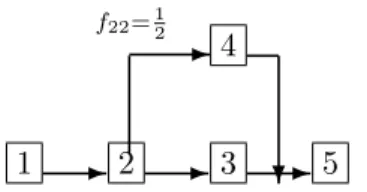
Figure 1: A 5-task project schedule for section 4.

¶ Consider the 5-task project shown in ﬁg. 1. This project has two task-paths: Path 1: 1 −→ 2 −→ 3 −→ 5

Path 2: 1 −→ 2 −→ 4 −→ 5

In path 2, task 4 is initiated when task 2 is half ﬁnished, as indicated byf22= 0.5.

¶ Nominal task durations. •For tasks 1, 2 and 5:

e

t1=te2 =et5 = 1, (16)

•Estimated durations of tasks 3 and 4 depend on allocation of a resource: q3 = resource allocated to task 3.

q4 = resource allocated to task 4.

Budget constraint:

1 =q3+q4 (17)

•More resource decreases estimated task durations:

e

t3 = 1−q3 =q4 (18)

e

t4 = 1−q4 (19)

Let q=q4 be a parameter which the project manager is free to choose in the interval [0,1].

¶ Theuncertainty in the actual task durations is represented by fractional-error info-gap model:

U(α,et) = { t: |tn_e−etn| tn ≤αwn, n= 1, . . . ,5 } α≥0 (20)

(14)

4.3 Project Reliability with a Global Time Buffer: Theory ¶ Consider a project whose task flow chart is shown in fig. 1, p. 13. This project has 2 task paths as indicated earlier.

¶ In order to answer the questions in section 4.2 we need: •Dynamic model: describing the task-path structure

and its relation to total project duration. •Failure criterion.

•Uncertainty model.

¶ We ﬁrst consider the dynamic model.

tn= unknown duration ofnth task, n= 1, . . . , N.

t= (t1, . . . , tN)T

There are M paths.

fmn= fractional participation of task nin pathm.

m: path. n: task.

In pathm, the task following taskn

begins when tasknis fraction fmn complete.

¶ E.g., in path 2 of ﬁg. 1:

task 4 begins when task 2 is 1/2 complete: f22= 0.5.

(15)

¶ The duration of the mth path, cm,

equals the sum of the durations ofall tasks

weighted by their fractional participations in pathm:

cm = N ∑ n=1

fmntn, m= 1, . . . , M (21)

For instance, the duration of the 2nd path is: c2= 1·t1+

1

2 ·t2+ 1·t4+ 1·t5 (22)

¶ DeﬁneF = matrix of participation factorsfmn ∈ ℜM×N.

For instance, for ﬁg. 1:

F = ( 1 1 1 0 1 1 1₂ 0 1 1 ) (23)

¶ Now the relation between task- and path-durations is:

c=F t (24)

¶ Thedynamic model is the duration of the longest path:

T =∥c∥= max 1≤m≤M|cm|=1≤maxm≤M N ∑ n=1 fmntn (25)

Note that∥c∥ is in fact a vector norm, sometimes called the “zero norm”.

¶ Thefailure criterion:

the project fails if the duration of the longest path exceeds a critical value:

T > tc (26)

¶ Uncertainty model: weighted fractional variations of task times.

U(α,et) = { t: |tn−_e etn| tn ≤wnα, n= 1, . . . , N } , α≥0 (27)

This is an unbounded family of nested sets. Two levels of uncertainty:

•At ﬁxed α: tn,n= 1, . . . , N are uncertain. e

(16)

•α, theuncertainty parameter, is unknown.

¶ Robustness function:

b

α = max α which precludes failure (29)

= max{α: failure is not possible} (30) = max { α: T ≤tc for all t∈ U(α,et) } (31) = max            α : max 1≤m≤M N ∑ n=1 fmntn | {z } cm ≤tc for all t∈ U(α,et)            (32) = max { α: ( max t∈U(α,et) max 1≤m≤M N ∑ n=1 fmntn ) ≤tc } (33)

¶ We can decompose this according to the separate paths:

b αm = robustness of pathm (34) = max { α : ( max t∈U(α,et) cm(t) ) ≤tc } (35)

¶ The project robustness is the lowest path-robustness:

b

α = min

1≤m≤Mαbm (36)

¶ Analyze the maximum ontin eq.(35): Recall that, for t∈ U(α,et):

e tn−wnetnα≤tn≤ten+wnetnα (37) Thus: max t∈U(α,et) cm = max t∈U(α,et) N ∑ n=1 fmntn (38) = N ∑ n=1 fmn ( e tn+wnetnα ) (39) = N ∑ n=1 fmnetn | {z } cm +α N ∑ n=1 fmnwnetn | {z } fm (40) = cm+αfm (41)

¶ The robustness of themth path is obtained by solving for α:

(17)

which is: b αm = tc−cm fm (43)

¶ As noted in eq.(36), the project robustness is the lowest path-robustness:

b α = min 1≤m≤Mαbm (44) = min 1≤m≤M tc−cm fm (45)

(18)

4.4 Robustness of the 5-Task Project

¶First consider therobustness function. In this problem the uncertainty weightswnare all equal

to unity, so the robustness of task-path m, eq.(43), is:

b αm = tc−ecm e cm (46) where e cm= N ∑ n=1 fmnetn (47)

The robustness is:

b

α= min

m αbm (48)

The participation matrix is:

F = ( 1 1 1 0 1 1 1₂ 0 1 1 ) (49) Hence: e c1 = et1+et2+q+et5 = 3 +q (50) e c2 = et1+ 1 2et2+ 1−q+et5= 3.5−q (51) So the path robustnesses are:

b α1(q) = tc 3 +q −1 (52) b α2(q) = tc 3.5−q −1 (53)

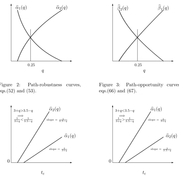
¶ We see that αb1(q) decreases monotonically with q while αb2(q) increases monotonically with q, as

shown schematically in ﬁg. 2. The overall robustness will be the lesser of these two functions at any value of q. That is, from this it is evident that the project robustness is:

b α= { b α2(q) , 0≤q ≤0.25 b α1(q) , 0.25≤q ≤1 (54)

Consequently we will choose q to maximizeαb:

b

qc= 0.25 (55)

¶Figs. 4 and 5 provide additional insight into why the robust-optimal allocation,qbc, occurs when the

path robustnesses are equal. By increasing the robustness of the more vulnerable path one necessarily reduces the robustness of the more immune path. The maximum project robustness occurs when the two path robustnesses are equal.

(19)

-6αb1(q) αb2(q) 0.25 q -6_βb 2(q) βb1(q) 0.25 q

Figure 2: Path-robustness curves, eqs.(52) and (53).

Figure 3: Path-opportunity curves, eqs.(66) and (67). -6 b α1(q) b α2(q) 3+q>3.5−q =⇒ 1 3+q< 1 3.5−q slope = 3.51−q slope = 1 3+q 0 tc -6 b α2(q) b α1(q) 3+q<3.5−q =⇒ 1 3+q> 1 3.5−q slope = 3+1q slope = 1 3.5−q 0 tc

Figure 4: Path-robustness curves vs. completion time tc, eqs.(52) and (53).

Figure 5: Path-robustness curves vs. completion time tc, eqs.(52) and (53).

¶ Note that the path robustnesses shown in ﬁgs. 4 and 5 become zero for speciﬁc values of required completion time tc. This means that the project robustness vanishes for some value of tc. One can

show that:

b

α(q, tc) = 0 if tc=T[et(q)] (56)

e

t(q) is the vector of anticipated task-completion times, and T[et(q)] is the anticipated project com-pletion time. What eq.(56) means is that one cannot rely upon attaining the anticipated comcom-pletion time. Only longer, less ambitious, completion times have robustness to task-time uncertainty.

¶Eq.(56) is true forany allocationq. In particular, eq.(56) holds for the allocation which minimizes the anticipated completion time:

q⋆ = arg min

q T[et(q)] (57)

Allocationq⋆ is the “best” decision based on the “best” model, but its performance has zero robust-ness to uncertainty. Only “sub-optimal” allocations have positive robustrobust-ness.

(20)

4.5 Opportuneness Analysis of the 5-Task Project ¶ Now consider theopportuneness function.

¶ The opportuneness for task-path mis:

b β_m = min { α: min t∈U(α,et) cm(t)≤tw } (58)

This is to be contrasted with the robustness of task-path m:

b αm= max { α: max t∈U(α,et) cm(t)≤tc } (59)

¶ Can we use the info-gap model in eq.(20)? No. We must assure that task-durations are non-negative. Thus we need the following modiﬁcation:

U(α,et) = { t: max[0, etn(1−α)]≤tn≤ten(1 +α), n= 1, . . . ,5 } α≥0 (60) ¶ Note that: max[0, ten(1−α)] = { 0, α ≥1 e tn(1−α), α ≤1 (61)

So it is evident that the opportuneness function will be less than βb= 1, since at uncertainty α = 1 each task could complete in zero time.

¶ Calculating minimal path duration at horizon of uncertaintyα:

min t∈U(α,et) cm(t) = min t∈U(α,et) N ∑ n=1 fmntn (62) = N ∑ n=1 fmnten(1−α) (63) = ecm−αecm (64)

Equating this to tw we see that the opportunity of path m is:

b β_m= cem−tw e cm = 1− tw e cm (65)

unless this is negative, in which case βb= 0. Explanation: eq.(65) is negative if cem−tw <0 which

means that the nominal duration is less than the windfall duration. In that case, the immunity to windfall is zero.

¶ The path opportunenesses are:

b β₁(q) = 1− tw 3 +q (66) b β₂(q) = 1− tw 3.5−q (67)

(21)

The overall opportuneness of the project is: b β= max m b β_m (68)

¶ We see that βb₁(q) increases monotonically with q while βb₂(q) decreases monotonically with q as shown schematically in ﬁg. 3. The overall opportunity will be the greater of these two functions at any value of q. That is, from this it is evident that the project opportunity is:

b β= { b β₂(q) , 0≤q≤0.25 b β₁(q) , 0.25≤q≤1 (69) Consequently we will chooseq to minimizeβbwhich, as for the robustness function, leads to the same optimum:

b

(22)

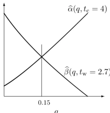
¶ Table 1 shows someαb andβbvalues. Recall thatαb is the greatest fractional error in task-duration which the project can tolerate, in each task, without time over-run, while βb is the smallest ‘error’ (early task completion) which the project needs, in each task, to enable windfall project completion. • Note that, in table 1 and (schematically) in ﬁg. 6, βb(q)≤αb(q) for all q ≤0.25 when tw = 3. This

means that the system can tolerate uncertainty at a level which facilitates windfall.

•However, in table 1 and (schematically) in ﬁg. 7, the robustness and opportuneness curves cross at q = 0.15 whentw = 2.7. That is,βb(q)>αb(q) forq <0.15. This means that, atq <0.15, the project

cannot tolerate the uncertainty needed to facilitate windfall. q αb=αb2 βb=βb2 βb=βb2 tc= 4 tw = 3 tw = 2.7 0.00 0.14 0.14 0.23 0.05 0.16 0.13 0.22 0.15 0.19 0.10 0.19 0.25 0.23 0.077 0.17

Table 1: Robustness and opportunity for various resource allocations.

-6 b β(q, tw = 3) b α(q, tc= 4) q -6 b β(q, tw= 2.7) b α(q, tc= 4) 0.15 q

Figure 6: Robustness and opportune-ness curves, withtc= 4 and tw = 3.

Figure 7: Robustness and opportune-ness curves, with tc= 4 and tw = 2.7.

(23)

5 Project Cost Management

¶ Project cost management: the PMI perspective9:

•Assure the project is completed within the approved budget. •Major processes for cost management:

◦Planwhat resources (people, equipment, materials) and what quantities are needed for implementing the project tasks.

◦ Estimatethe cost of the required resources. ◦ Allocatebudget to individual tasks.

◦ Control changes in the project budget.

¶ What are the info-gaps in cost management? •Unanticipated resource needs.

•Unanticipated resource costs.

•Both needs and costs are projections from the past to the future.

•Unanticipated budget constraints due to changing corporate plans and capabilities.

¶ Info-gap models of uncertainty:

•c(t) = the cost of a resource over the life of the project.

•We will consider three info-gap models for uncertainty in this function: ◦ Envelope-bound model.

◦ Slope-bound model.

◦ Fourier ellipsoid-bound model.

•Before studying the Fourier ellipsoid model, we will review: ◦ Fourier representation of a function.

◦ Matrix representation of ellipsoids.

9

(24)

5.1 Envelope-Bound Info-gap Model of Uncertainty ¶ Prior information:

•ce(t) = best known estimate of the cost function. •c(t) = unknown true cost function.

•Large costs tend to have large ﬂuctuations.

¶ The envelope-bound info-gap model for uncertainty in the scalar cost functionc(t):

U(α,ec) = { c(t) : c(t)−ec(t) e c(t) ≤α } , α≥0 (71)

• U(α,ce),α≥0, obeys nesting and contraction.

• U(α,ce) is analog of fractional-error info-gap model, eq.(5), p.5 and eq.(10), p.7.

¶ Alternative prior information:

•ψ(t) = shape of envelope-of-ﬂuctuation. Perhaps seasonal.

¶ The envelope-bound info-gap model for uncertainty in the scalar cost functionc(t):

U(α,ce) ={c(t) : |c(t)−ec(t)| ≤αψ(t)}, α≥0 (72) •Eq.(71) is special case of eq.(72) with ψ(t) =ce(t).

(25)

5.2 Slope-Bound Info-gap Model of Uncertainty

¶ Envelope-bound info-gap model allows unbounded rate of variation. •Sometimes we know the rate of variation is constrained. •We will consider two info-gap models:

◦ Slope-bound model.

◦ Fourier ellipsoid-bound model (section 5.5).

¶ Prior information:

•Rate of deviation ofc(t) fromce(t) is bounded. •Bound is unknown.

¶ The slope-bound info-gap model for uncertainty in the scalar cost function c(t):

U(α,ec) = { c(t) : d[c(t)−ce(t)] dt ≤α } , α≥0 (73)

(26)

5.3 Fourier Representation of a Function ¶ We now review the Fourier representation of a function.

We will use Fourier representations in a new type of info-gap model.

¶ Let ϕ(x) be an arbitrary but piece-wise continuous function deﬁned on the interval −L≤x≤L. Then ϕ(x) can be represented as:

ϕ(x) = ∞ ∑ n=0 [ bnsin nπx L +cncos nπx L ] (74)

¶ Let ϕ(x) be an arbitrary but piece-wise continuous function deﬁned on the interval 0 ≤ x ≤ L. Then ϕ(x) can be represented as:

ϕ(x) = ∞ ∑ n=0 cncos nπx L (75)

¶ How to choose the Fourier coeﬃcients c0,c1, . . . ?

Exploit orthogonality: ∫ _π 0 cosmxcosnxdx= { π 2 m=n 0 m̸=n (76)

Multiply both sides of eq.(75) by coskπx_L and integrate from 0 to L:

∫ _L 0 ϕ(x) coskπx L dx = ∞ ∑ n=0 cn ∫ _L 0 coskπx L cos nπx L dx (77) = ckL 2 (78)

So, if we know the function ϕ(x) we can calculate the Fourier coeﬃcients of its expansion:

ck= 2 L ∫ _L 0 ϕ(x) coskπx L dx (79)

(27)

¶ Band-limited function: ϕ(x) = n2 ∑ n=n1 cncos nπx L (80) = cTγ(x) (81)

¶ Uncertainty inϕ(x) is represented as uncertainty in Fourier coeﬃcients c. •For instance: cin ellipsoid of known shape and unknown size:

U(α,ce) =

{

ϕ(x) =cTγ(x) : (c−ce)TW(c−ec)≤α2

}

, α≥0 (82)

¶ These Fourier coeﬃcients have many interesting and important properties.

•First of all, they minimize the mean squared error between ϕ(x) and its expansion. That is, thecnminimize: S2= ∫ _L 0 ( ϕ(x)− ∞ ∑ n=0 cncos nπx L )2 dx (83) In fact, lim N→∞S 2 _{= 0} ₍₈₄₎

•Another important property relates to truncated expansions:

ϕ(x) = N ∑ n=0 cncos nπx L dx (85)

Regardless of the order of the expansion, N:

◦ Orthogonality yields the same Fourier coeﬃcients, ck.

◦ These coeﬃcients minimize the mean squared error of the truncated expansion.

(28)

5.4 Geometry of Ellipsoids

¶ We need one more digression before we proceed to the new info-gap model: Geometry of ellipsoids.

¶ Thequestion we study in this subsection is: What are the directions and lengths of the principal axes of an ellipsoid?

¶ If: c is anN-vector and

W is a real, symmetric, positive deﬁnite matrix, then an ellipsoid of c-vectors of dimensionN is deﬁned by:

cTW c=r2 (86)

where r is any positive real number.

¶ To answer our question, we must solve an optimization problem. We must ﬁnd vectorscwhich have two properties:

•Length is extremal.

•Lie on the boundary of the ellipsoid.

¶ To solve this problem we will use the method of Lagrange multipliers.

¶ To optimize the length ofc, it is suﬃcient to optimize the square of the length of c. So we must optimize:

cTc (87)

¶ Ac-vector lies on the ellipsoid if eq.(86) is satisﬁed. Expressing this slightly diﬀerently, the constraint on c is:

r2−cTW c= 0 (88)

¶ Deﬁne the objective function:

H =cTc−λ(r2−cTW c) (89) If we ﬁnd all c-vectors which optimizeH subject to the constraint,

we will have solved the problem. ¶ Condition for extremum ofH:

0 = ∂H

∂c = 2c−2λW c (90)

=⇒ (I−λW)c= 0 (91)

which means that:

c= is an eigenvector ofW. 1

(29)

¶ Deﬁne the eigenvalues and orthonormal eigenvectors ofW:

W vi =µivi, i= 1, . . . , N (92)

where:

0< µ1 ≤ · · · ≤µN and vmTvn=δmn (93)

where δmn is the Kronecker delta function:

δmn= {

1 m=n

0 m̸=n (94)

¶ Now, since cmust be an eigenvector ofW, we know that:

c=hvi (95)

for some non-zero h and for anyi= 1, . . . , N. Hence the constraint on cis:

r2 =cTW c=h2v_iTW vi=h2µi =⇒ h=±

r √_µ

i

(96) ¶ Thus the optimizingc-vectors are:

c=±√r µi

vi, i= 1, . . . , N (97)

From this we see that:

The directions of the principal semi-axes are:

±v1, . . . , ±vN (98)

The lengthsof the principal semi-axes are: r √_µ 1 , . . . ,√r µN (99)

(30)

5.5 Fourier Ellipsoid-Bound Info-gap Model of Uncertainty

¶ We now consider a diﬀerent type of prior information about the uncertain cost functionc(t). ¶ About c(t) we know:

•ce(t) is the known best estimate of the cost function. •c(t) is the unknown true cost function.

•c(t)−ec(t) is error of the estimated cost function. •c(t)−ec(t) is constrained to speciﬁc known frequencies. •The amplitudes of these frequencies are bounded

by an ellipsoid of known shape. ¶ About c(t) we do not know:

•The precise amplitudes of the Fourier coeﬃcients. •The size of the ellipsoid.

¶ In other words, the cost function is represented by:

c(t) = ec(t) + n2 ∑ n=n1 bnsin nπx L (100) = ec(t) +bTσ(x) (101) where:

b= vector of unknown Fourier coeﬃcients.

σ(x) = vector of known corresponding sine functions.

¶ The uncertainty inc(t) is represented by the following Fourier ellipsoid bound info-gap model: U(α,ce) =

{

c(t) =ec(t) +bTσ: bTW b≤α2

}

, α≥0 (102)

(31)

6 Project Quality Management

¶ Project quality management: the PMI perspective10:

•Ensure the project will satisfy the needs for which it was undertaken. •Major quality management processes:

◦ Planning: identify the quality standards relevant to the project and determine the means of satisfying them.

◦ Assurance: Evaluate the project performance on a regular basis to determine that the project will satisfy the quality standards.

◦ Control: Monitor speciﬁc project results and determine if they satisfy quality require-ments. Determine means to eliminate unsatisfactory performance.

¶ Where are the info-gaps in quality management? •Standards change during the life of the project.

•Technology for compliance become obsolete and unavailable.

•Periodic evaluations of project quality provide inaccurate forecasts of ﬁnal project compliance with quality standards.

•Workers or sub-contractors falsify quality reports. •Means to rectify quality short-falls are infeasible.

10

(32)

7 Project Human Resource Management

¶ Project human resource management: the PMI perspective11:

• “Processes required to make the most eﬀective use of the people involved in the project.” This includes all stakeholders: sponsors, customers, partners, individuals, and others.

•Major processes are:

◦ Organizational planning: identify, document and assign roles and responsibilities. ◦ Staﬀ acquisition: get the human resources needed for the project.

◦ Team development: develop individual and group skills needed for the project.

¶ Where are the info-gaps in human resource management?

•Inaccurate identiﬁcation of roles and responsibilities needed for the project. •Inappropriate assignment of responsibilities.

◦This may result from asymmetric information: the prospective employee does not reveal his true abilities and propensities.

◦ This may result from inaccurate understanding of responsibilities. •Incomplete training, or excessive training in unneeded areas.

11

(33)

8 Project Communications Management

¶ Project communications management: the PMI perspective12:

• Ensure “timely and appropriate generation, collection, dissemination, storage, and ultimate disposition of project information.”

•Provide “critical links among people, ideas, and information that are necessary for success.” •Major processes for communications management:

◦ Communications planning: determine “the information and communications needs of the stakeholders: who needs what information, when they will need it, and how it will be given to them.”

◦ Information distribution: make “needed information available to project stakeholders in a timely manner.”

◦ Performance reporting: Collect and disseminate performance information: status re-ports, progress measurements, forecasts.

◦ Administrative closure: generate, gather, and disseminate information to formalize a phase or project completion.

¶ Where are the info-gaps in communications management?

•Inaccurate or incomplete assessment of stakeholder informational needs. ◦ Too much information is distributed.

◦ Too little information is distributed. •Information channels are too noisy or too slow. •Information collection and processing is inaccurate. •Information is deliberately corrupted.

12

(34)

9 Project Risk Management

¶ Project risk management: the PMI perspective13: •Identify, analyze and respond to project risk. •This includes:

◦ Maximize “probability and consequences of positive events”. ◦ Minimize “probability and consequences of adverse events”. ◦ Maximize robustness of project to:

— Adverse events. — Information-gaps.

◦ Minimize immunity of project to opportune events. •Major processes in risk management:

◦ Risk management planning: decide “how to approach and plan the risk management of activities for a project.”

◦ Risk identiﬁcation: determine “which risks might aﬀect the project”.

◦ Qualitative risk analysis: perform “a qualitative analysis of risks and conditions to prioritize their eﬀects on project objectives.”

◦ Quantitative risk analysis:

— Measure “the probability and consequences of risks” and estimate “their im-plications for project objectives.”

— Evaluate robustness to info-gaps.

— Evaluate opportuneness from uncertainty.

◦ Risk response planning: develop “procedures and techniques to enhance opportunities and reduce threats to the project’s objectives.”

◦Risk monitoring and control: monitor existing risks, identify new risks, implement risk reduction plans.

¶ Where are the info-gaps in risk management?

•A risk is a factor which can adversely aﬀect the project outcome. ◦ Risk is aninput to the project whoseoutput is detrimental. ◦ Predicting outputs can be uncertain.

— It may depend on an inaccurate model of the project. — It may require large and unavailable resources. •Not all risk factors are identiﬁed or accurately quantiﬁed.

•Measurement and monitoring of risks and their consequences may be inaccurate or incomplete. •Responses to risks may be inadequate or infeasible.

13

(35)

10 Project Procurement Management

¶ Project procurement management: the PMI perspective14:

•Includes “the processes required to acquire goods and services, to attain project scope, from outside the performning organization.”

•Major procurement processes:

◦ Procurement planning: determine what to procure and when.

◦ Solicitation planning: document requirements and identify potential sources. ◦ Solicitation: obtain bids, oﬀers, etc.

◦ Source selection: choose among potential sources.

◦ Contract administration: manage relationships with sources. ◦ Contract closeout: complete and settle contracts.

¶ Where are the info-gaps in procurement management? •Required goods may not be known far in advance.

•Potential sources may vanish; new ones may appear.

•Bids may be unrealistic; source may not be able to provide according to oﬀer. •Time delays in provision of goods.

•Cost over-runs and bankruptcy of suppliers.

14

Lecture Notes on Info-gaps in Project Management Knowledge Areas

Info-gaps in Project Management Knowledge Areas

Contents

1

Project Integration Management

2

Project Scope Management

3

Project Time Management

4

Example: Managing Task-Duration Uncertainty

5

Project Cost Management

6

Project Quality Management

7

Project Human Resource Management

8

Project Communications Management

9

Project Risk Management

10

Project Procurement Management