174
© Global Society of Scientific Research and Researchers http://asrjetsjournal.org/
The Use of Group Method of Data Handling and
Multilayer Perceptron Neural Network for the Prediction
of Significant Wave Height
Moussa S. Elbisy*
Civil Engineering Dept., College of Engineering and Islamic Architecture, Umm Al-Qura University, Makkah, Saudi Arabia
Email: [email protected]
Abstract
The prediction of significant wave height is important in the planning, design, and operation of coastal and ocean structures. Although several empirical methods, numerical models, and soft-computing techniques to forecast wave parameters have been investigated, such forecasting still remains a complex problem in the field of ocean engineering. This study uses the group method of data handling-type neural network (GMDH-NN) and multilayer perceptron neural network (MLPNN) to predict significant wave height. Among the used models, the GMDH-NN is found to provide the best generalization capability and the lowest prediction error; therefore, this is the method that can be most successfully used to predict significant wave height.
Keywords: Prediction; Group Method of Data Handling; multilayer perceptron; significant wave height.
1.Introduction
It should be noted that the prediction of sea-wave parameters plays an important role in various ocean engineering tasks, such as the design of marine structures like oil platforms or harbors and the design and management of marine energy systems like wave energy converters, among others [1-2]. Therefore, several models and approaches, such as empirical methods, numerical models, and soft-computing techniques, have been proposed to predict sea-wave parameters.
--- * Corresponding author
175
Comparing the forecasting results of neural networks (NNs) and auto-regressive models, the authors in [3] reported NN models to be more accurate. Deo and his colleagues in [4] tested a feed-forward neural network (FFNN) to obtain significant wave heights and average wave periods using wind speed values of current and previous time steps as input. The authors in [5], on the other hand, predicted wave heights using a back-propagation neural network (BPNN), a cascade-correlation neural network (CCNN), and auto-regressive models (ARMA and ARIMA). These authors found NNs to be more accurate than the auto-regressive methods. Tsai and his colleagues in [6] used a BPNN to forecast ocean waves based on the learning characteristics of the observed waves and wave records at neighboring stations. The author in [7] applied the FFNN technique to predict significant wave heights and zero-up-crossing wave periods over hourly intervals from 1 h to 24 h. The authors in [8] forecasted wave heights and zero-up-crossing wave periods at intervals of 3, 6, 12 and 24 h using an FFNN. The authors in [9] used a recurrent neural network to forecast the significant wave height on the west coast of India. The authors in [10] compared NNs, FISs and ANFISs in hindcasting wave parameters. Their results showed that these methods perform nearly the same. According to the meteorological data, the author in [11] predicted monthly mean significant wave heights by using NN and regression methods. The author in [12] used support vector machine (SVM) approach with various kernel functions for wave parameters prediction. The SVM results are compared with the field data and with BPNN and CCNN models. The results indicated that the SVM with a radial basis function kernel provides the best generalization capability and the lowest prediction error. The authors in [13-15] combined NN and numerical models to realize the wave height prediction. The authors in [16] used recurrent neural networks (RNN) for wave prediction based on the data gathered and the measurement of the sea waves in the Caspian Sea, in the north of Iran. The authors in [17] used nonlinear regression and SVM methods to predict significant wave height. The results explained that the use of nonlinear regression methods gave a good result compared to the results from support vector machine. The results indicated that support vector machine based on radial basis function is more superior to nonlinear regression methods. The aim of the present study is to illustrate a new approach to predict significant wave height using the Group Method Data Handling type neural network (GMDH-NN) and Multi-layer Perceptron Neural Network (MLPNN). The manuscript is organized as follows: the next section introduces the methods used in this study. Section 3 describes the studied area and the data used. Section 4 presents the results of the GMDH-NN and MLPGMDH-NN methods. The conclusions are reported in the final section.
2.Methods
2.1.Group method of data handling neural network
The Group Method of Data Handling (GMDH) type neural network (NN) is a powerful identification technique and can be used to model complex systems, where unknown relationships exist between variables, without having specific knowledge of processes. GMDH is a kind of machine learning algorithm where an artificial neural network algorithm is built heuristically using self-organization method. Originally GMDH-type neural network algorithms are applied to predict and forecast a univariate time series GMDH finds its applications in a wide spectrum of areas, ranging from prediction, forecasting, data mining, systems modelling, pattern recognition and knowledge discovery. GMDH algorithms are generally inductive that offer possibility to manage interrelations among data automatically. Its most powerful feature is the ability to select an optimal complexity of the neural network structure while achieving the maximum possible prediction accuracy. Once an
176
optimal complexity of the neural network structure is found, the prediction model is quite resistant to noise in data sample. In data mining, the model avoids over-fitting and under-fitting, where noise in the data would no longer pose problem of performance degradation. The neural network structure is therefore simplified yielding an optimal model that is just sufficient in the amounts of neurons and hidden layers to maintain its maximum possible accuracy. GMDH-NN is a self-organizing approach by which more complicated models are gradually generated based on the evaluation of their performance on a set of multi-input, single-output data pairs This approach was proposed by Ivakhnenko in the 1960s. It has a series of operations, such as seeding, rearing, crossbreeding, and selection and rejection of seeds corresponding to the determination of the input variables, the structure and parameters of the model, and the selection of the model by the principle of termination [18]. The typical GMDH algorithm can be represented as a set of neurons in which different pairs of them in each layer are connected through a quadratic polynomial and thus produce new neurons in the next layer [19]. General connection between inputs and output variables can be expressed by a complicated discrete form of the Volterra functional series in the form of [20]:
∑ ∑ ∑ ∑ ∑ ∑ (1)
Which is known as the Kolmogorov–Gabor polynomial, where ( )is the input vector, and
y is the output variable. GMDH works by building successive layers with complex links that are the individual terms of a polynomial. The initial layer is simply the input layer. The first layer created is made by computing regressions of the input variables and then choosing the best ones. The second layer is created by computing regressions of the values in the first layer along with the input variables. This means that the algorithm essentially builds polynomials of polynomials.
2.2.Multi-perceptron neural network
As the name implies, an MLPNN can have several layers. Each layer has a weight matrix, a bias vector, and an output vector. The MLPNN architecture contains an input layer, an output layer and at least one hidden layer, which are all fully interconnected. The network is repeatedly exposed to a set of training data, and errors are calculated based on the resulting outputs. These errors are used to adjust the weights and biases. This process will eventually lead to optimum and bias values that can mimic of the model. The transfer functions (logistic (sigmoid) and linear) are used as activation function for the hidden layers and the output layer, respectively. A wide range of parameters, such as the number of layers and neurons of each layer, initial conditions and learning factor, can affect the network’s performance.
2.3. Model assessment
The performance of all GDMH-NN and MLPNN models were assessed based on calculating the normalized mean square error (NMSE), the correlation coefficient (R), the root mean square error (RMSE), the mean squared error (MSE), the mean absolute error (MAE), and the mean absolute percentage error (MAPE). The six statistical parameters used to compare the performance of various GDMH and MLPNN configurations are:
177
∑ ( ) (2) ∑ ( )( ) √∑ ( ) ∑ ( ) (3)
N i i i O P N RMSE 1 2 1 (4) ∑ ( ) (5)
N i i i O P N MAE 1 1 (6) 100 ) ( 1 1
N i i i i P O P N MAPE (7)Where Oi is the observed value, Pi is the predicted value, N is the total number of data points in validation,
O is the mean value of the observations, and P is the mean value of the predictions.
3.Study Area and data
The study area is the Abu Qir Bay coastal zone, a semi-circular basin that lies approximately 35 km northeast of Alexandria on the north-eastern Egyptian Nile delta coast, between latitude 31°16' and 31°28'N and longitude 30°4' and 30°20'E. Wind data (speed and direction), taken during 2010 to 2014 from a weather station at the Abu Qir Bay, are sampled at 6-hour intervals and calculated at 10 m above sea level. The collected wind data are subjected to statistical analysis to determine the percentage of occurrence of a certain wind speed moving in a certain direction. The waves were measured using a Cassette Acquisition System (CAS) directional wave recorder during 2010 to 2014. The system is a portable, self-contained remote recording system for sensing near-shore environmental parameters, such as wave height, wave direction and wave period. This device was fixed on a gas platform in Abu Qir Bay at 31°24' N latitude and 30°14' E longitude. The water depth at this location was 18m. The system's sensors made four recordings a day (every 6 hours) that lasted approximately 34 minutes. The wave data were recorded on cassettes and analysed. The fetch length in a certain direction was determined by constructing 30 radials from the point of interest (at 1° intervals) and extending them until they intersected the coastline. Next, the fetch length was calculated as the arithmetic average of the extended radials.
4.Results and discussion
The GMDH-NN and MLPNN were applied, based on the observations. The wind speeds (U) and fetch (F) were selected as the input variables to the models. The output is the significant wave height (Hs). A certain amount of data processing is required before presenting the training patterns to the network. In this study a linear scaling was used. A linear normalization function within the values of zero to one is:
178
( ()) ( ⁄ )
(8)
Where S is the normalized value of variable V, Vmin and Vmax are variable minimum and maximum values
respectively.
4.1. MLPNN
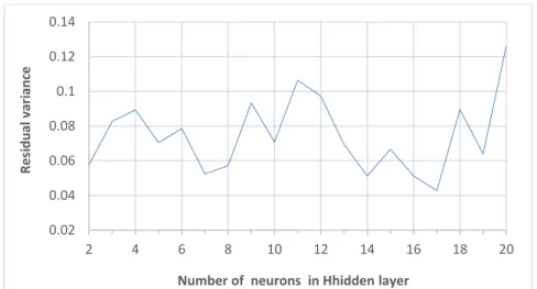
Genetic Algorithm (GA) was utilised to adjust the MLPNN model to its optimised performance. The GA tests different combinations of different parameters. This process is repeated for each solution in a generation, so that new generation are ameliorated compared to their predecessors. The network parameters tested in the proposed model included the following: the number of hidden layers, the number of hidden neurons, the learning rate, the momentum factor, the input noise and the training time. Integrated performance testing indicated the following best network parameters: the number of hidden layers was two, the number of neurons in the first hidden layer was two, the number of neurons in the second hidden layer was seventeen, the learning rate was 0.75, the momentum factor was 0.31, and the input noise was 0.016. Model results for different MLPNN architectures are presented in Figure (1) which shows the performance of the MLPNN with various numbers of neurons in one hidden layer.
Figure 1: The performance of the MLPNN with numbers of neurons in hidden layer.
Table 1 shows the error statistics for the observed and predicted significant wave heights. The values for the
NMSE, MAE, MSE, RMSE, MAPE and R of the wave height MLP prediction model are 0.0001 m, 0.00836 m, 0.00021 m2, 0.01441 m, 19.366 and 0.99, respectively. The results show that the MLP model significantly reduces overall error. The correlation between the observed and predicted values for Hs by the MLP model is
shown in Figure (2). Figure (3) presents the rresidual error between observed and predicted Hsfor MLP (2–17– 1) model. 0.02 0.04 0.06 0.08 0.1 0.12 0.14 2 4 6 8 10 12 14 16 18 20 R e si d u al v ar ian ce
179
Figure 2: Scatter of predicted observed values of Hs for MLPNN model.
Figure 3: Residual error between observed and predicted Hs for MLPNN model.
Table 1: Error statistics for the observed and predicted Hs by the GMDH-NN and MLPNN models.
Model Error statistics
NMSE (m) MAE (m) MSE (m2) RMSE (m) MAPE (%) R
GMDH-NN 9.7717x10⁻⁶ 0.0029 1.5493 x10⁻⁵ 0.0039 3.6752 0.99
MLPNN 0.0001 0.0084 0.0002 0.0144 19.366 0.982
4.2.GMDH-NN
As mentioned in the GMDH-NN definitions section, structure of the GMDH-NN model is built using least square sense. In the present study, Quadratic polynomial neurons extracted from the GMDH-NN model were expressed as, (9) 0 0.5 1 1.5 2 2.5 3 3.5 4 4.5 0 0.5 1 1.5 2 2.5 3 3.5 4 4.5 Pr e d ic te d H s Actual Hs -0.2 -0.1 0 0.1 0.2 0.3 0.4 0.5 0.6 0 5000 10000 15000 20000 25000 30000 35000 40000 R e si d u al E rr o r (m) Data No.
180
When the GMDH-NN model was applied, the NMSE was 9.7717x10⁻⁶, the MAE was 0.002879, the MSE was 1.54931 x10⁻⁵, the RMSE was 0.003936, and MAPE was 3.6752. Correlation coefficient of 0.999 was obtained. The results show that the GMDH-NN model significantly reduces overall error. The variation in Hs between the
observed data and the results of the GMDH-NN model has the same trend. Figure (4) illustrates the residual error between observed and predicted Hsfor GMDH-NN model. The correlation between the observed and predicted values for Hs by the GMDH-NN model is shown in Figure (5).
Figure 4: Residual error between observed and predicted Hs for GMDH-NN model.
Figure 5: Scatter of predicted observed values of Hs for GMDH-NN model.
4.3.Comparison between GMDH-NN and MLPNN
According to the indices, the GMDH-NN model can significantly reduce the overall forecasting errors and produced the best performance and was able to accurately estimate the wave heights. A comparison of the results of the GMDH-NN model and the MLPNN model shows that the percentage improvements in MAE,
RMSE, and MAPE of the GMDH-NN model over the MLPNN model were 65.48%, 72.92%, and 81.02% for predicting Hs, respectively. The prediction accuracies of the GMDH-NN model and the MLPNN model for
-0.05 -0.03 -0.01 0.01 0.03 0.05 0 10000 20000 30000 40000 R e si d u al E rr o r (m) Data No. 0 0.5 1 1.5 2 2.5 3 3.5 4 4.5 0 1 2 3 4 Pr e d ic te d H s Acual Hs
181
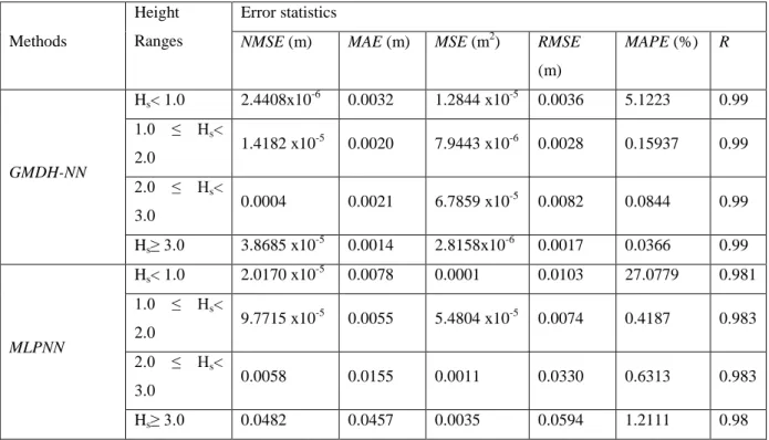
different wave height ranges are investigated. Table 2 shows that the GMDH-NN performed better than the MLPNN. According to the indices, the GMDH-NN model performs best for predicting Hs for all of the wave
height ranges. A comparison of the MAE values shows that the largest difference in the performance of the two methods, 96.94 %, is observed at wave heights more than 3.0 m, while the smallest difference (58.97%) is observed at wave heights less than 1.0 m. From Table 3, it can be seen that, in terms of MAPE, the largest performance difference for the two methods (96.98 %) is observed at wave heights more than 3.0 m, while the smallest difference (61.94%) is observed at wave heights from 1.0 to 2.0 m. A comparison of the RMSE values shows that the largest difference in the performance of the two methods, 97.14 %, is observed at wave heights more than 3.0 m, while the smallest difference (62.16%) is observed at wave heights from 1.0 to 2.0 m. From the results, it can be seen that the predictions of the GMDH-NN are closer to the corresponding actual values at all wave height ranges than for the MLPNN method. Generally, the GMDH-NN model forecasting results are more accurate than of the MLPNN. That is, the GMDH-NN model is capable of forecasting wave heights for different ranges. The notable point in this method is the self-organizing characteristic of the network and its high flexibility, making it a powerful instrument for prediction of a variety of nonlinear complex systems.
Table 2: Error statistics for the observed and predicted Hs by the MLPNN and GMDH-NN models for different height ranges.
Methods
Height Ranges
Error statistics
NMSE (m) MAE (m) MSE (m2) RMSE
(m) MAPE (%) R GMDH-NN Hs< 1.0 2.4408x10⁻⁶ 0.0032 1.2844 x10⁻⁵ 0.0036 5.1223 0.99 1.0 ≤ Hs< 2.0 1.4182 x10 -5 0.0020 7.9443 x10⁻⁶ 0.0028 0.15937 0.99 2.0 ≤ Hs< 3.0 0.0004 0.0021 6.7859 x10 -5 0.0082 0.0844 0.99 Hs≥ 3.0 3.8685 x10⁻⁵ 0.0014 2.8158x10⁻⁶ 0.0017 0.0366 0.99 MLPNN Hs< 1.0 2.0170 x10⁻⁵ 0.0078 0.0001 0.0103 27.0779 0.981 1.0 ≤ Hs< 2.0 9.7715 x10 -5 0.0055 5.4804 x10⁻⁵ 0.0074 0.4187 0.983 2.0 ≤ Hs< 3.0 0.0058 0.0155 0.0011 0.0330 0.6313 0.983 Hs≥ 3.0 0.0482 0.0457 0.0035 0.0594 1.2111 0.98 5.Conclusions
The accurate prediction of ocean wave parameters, for example, wave height and wave period, is of vital importance for project, design, use, and maintenance of structures in offshore and coastal engineering. In this paper, two types of prediction methods (GMDH-NN and MLPNN) were introduced and tested. The presented NN model provides lower forecasting error than do the MLP model. The results show that the GMDH-NN model outperformed the MLPGMDH-NN model. In conclusion, the S GMDH-GMDH-NN model has the highest accuracy
182
and better generalization performance than the MLPNN model for all wave height for different ranges. The results obtained in this investigation demonstrate that the GMDH-NN model is a promising alternative to MLPNN for significant wave height forecasting.
6.Recommendations
From the study, it is recommended to study the effect of sea level pressure and air temperature, and to relate their effect on the efficiency of the different soft computing models used for predicting significant wave height.
Acknowledgment
The author would like to express his high appreciation to the referees of the paper for their critical review as well as their valuable comments that improved the paper to its present form.
References
[1]. F. Comola, T. Lykke Andersen, L. Martinelli, H.F. Burcharth, and P. Ruol, “Damage Pattern and Damage Progression on Breakwater Roundheads under Multidirectional Waves.” Coastal Engineering, Vol. 83, pp. 24–35, 2014.
[2]. S.W. Kim, and K.D. Suh “Determining the Stability of Vertical Breakwaters Against Sliding Based on Individual Sliding Distances during a Storm.” Coastal Engineering, Vol. 94, pp. 90–101, 2014.
[3]. M.C. Deo, and C.S. Naidu “Real Time Wave Forecasting Using Neural Networks.” Ocean Engineering, Vol. 26, pp. 191-203, 1999.
[4]. M.C. Deo, A. Jha, A.S. Chaphekar, and K. Ravikant “Neural Networks for Wave Forecasting.” Ocean Engineering, Vol. 28, pp. 889–898, 2001.
[5]. J. D. Agrawal, and M. C. Deo “On-line wave prediction.” Marine Structures, Vol. 15, pp. 57–74, 2002. [6]. C.P. Tsai, C. Lin, and J. N. Shen “Neural Network for Wave Forecasting among Multi-Stations.” Ocean
Engineering, Vol. 29, pp. 1683-1695, 2002.
[7]. O. Makarynskyy “Improving Wave Predictions with Artificial Neural Networks.” Ocean Engineering, Vol. 31, No. 5–6, pp. 709–724, 2004.
[8]. O. Makarynskyy, A.A. Pires-Silva, D. Makarynska, and C. Ventura-Soares “Artificial Neural Networks in Wave Predictions at the West Coast of Portugal.” Comput. Geosci., Vol. 31, No. 4, pp. 415–424, 2005.
[9]. S. Mandal, and N. Prabaharan “Ocean Wave Forecasting Using Recurrent Neural Networks.” Ocean Engineering, Vol. 33, pp. 1401–1410, 2006.
[10]. J. Mahjoobi, A. Etemad-Shahidi, and M.H. Kazeminezhad “Hindcasting of Wave Parameters Using Different Soft Computing Methods.” Applied Ocean Research, Vol. 30, pp. 28–36, 2008.
[11]. K. Günaydın “The Estimation of Monthly Mean Significant Wave Heights by Using Artificial Neural Network and Regression Methods.” Ocean Engineering, Vol. 35, pp. 1406–1415, 2008.
[12]. M.S. Elbisy “Sea Wave Parameters Prediction by Support Vector Machine Using a Genetic Algorithm.” Journal of Coastal Research, Vol. 31, No. 4, pp. 892-899, 2015.
183
[13]. I. Malekmohamadi, R. Ghiassia, and M.J. Yazdanpanah “Wave Hindcasting by Coupling Numerical Model and Artificial Neural Networks.” Ocean Engineering, Vol. 35, pp. 417–425, 2008.
[14]. S.N. Londhe, and V. Panchang “One-Day Wave Forecasts Based on Artificial Neural Networks.” J. Atmos. Oceanic Tech- nol., Vol. 23, pp. 1593–1603, 2016.
[15]. A.N. Deshmukh, M.C. Deo, P.K. Bhaskaran, T.M. Balakrishnan Nair, and K.G.Sandhya “Neural-Network-Based Data Assimilation to Improve Numerical Ocean Wave Forecast.” IEEE J. Oceanic Eng., Vol. 41, pp. 944–953, 2016.
[16]. T. Sadeghifar, M.N. Motlagh, M.T. Azad, and M.M. Mahdizadeh, “Coastal Wave Height Prediction Using Recurrent Neural Networks (RNNs) in the South Caspian Sea.” Marine Geodesy, Vol.40, No. 2, pp. 454-465, 2017.
[17]. T. Elgohary, M.S. Elbisy, A.M. Mobasher, and H. Salah “Deep Wave Height Prediction for Alexandria Sea Region by Using Nonlinear Regression Method Compared to Support Vector Machines.” Current Development in Oceanography, Vol. 10, No. 1, pp. 1-14, 2018.
[18]. V. Garg “Inductive Group Method of Data Handling Neural Network Approach to Model Basin Sediment Yield.” J Hydrol Eng, Vol. 20, No. 6, C6014002, 2014.
[19]. N. Nariman-Zadeh, A. Darvizeh, M.E. Felezi, and H. Gharababaei “Polynomial Modelling of Explosive Compaction Process of Metallic Powders Using GMDH-type Neural Networks and Singular Value Composition.” Model. Simul. Mater. Sci. Eng., Vol. 10, No. 6, pp. 727-744, 2002.
[20]. F. Kalantary, H. Ardalan, and N. Nariman-Zadeh “An investigation on the Su–NSPT Correlation Using GMDH Type Neural Networks and Genetic Algorithms.” Eng Geol, Vol. 104, No. 1–2, pp. 44–55, 2009.