DOI 10.1007/s10951-006-0323-7
Cyclic preference scheduling of nurses using a Lagrangian-based
heuristic
Jonathan F. Bard·Hadi W. Purnomo
C
Springer Science + Business Media, LLC 2007
Abstract This paper addresses the problem of developing cyclic schedules for nurses while taking into account the quality of individual rosters. In this context, quality is gauged by the absence of certain undesirable shift patterns. The problem is formulated as an integer program (IP) and then decomposed using Lagrangian relaxation. Two approaches were explored, the first based on the relaxation of the pref-erence constraints and the second based on the relaxation of the demand constraints. A theoretical examination of the first approach indicated that it was not likely to yield good bounds. The second approach showed more promise and was subsequently used to develop a solution methodology that combined subgradient optimization, the bundle method, heuristics, and variable fixing. After the Lagrangian dual problem was solved, though, there was no obvious way to perform branch and bound when a duality gap existed be-tween the lower bound and the best objective function value provided by an IP-based feasibility heuristic. This led to the introduction of a variable fixing scheme to speed conver-gence. The full algorithm was tested on data provided by a medium-size U.S. hospital. Computational results showed that in most cases, problem instances with up to 100 nurses and 20 rotational profiles could be solved to near-optimality in less than 20 min.
J. F. Bard ()
Graduate Program in Operations Research & Industrial Engineering, 1 University Station C2200,
The University of Texas, Austin, TX 78712-0292, USA e-mail: [email protected]
H. W. Purnomo
American Airlines, AMR Corp Headquarter HDQ1, Mail Drop 5358, Fort Worth, TX 76155, USA
e-mail: [email protected]
Keywords Cyclic scheduling·Preference scheduling· Nurse rostering·Lagrangian relaxation·Bundle method
1 Introduction
The demand for nurses in the United States has been out-pacing the supply for more than a decade. The situation is now at the point where the rules for good practice are being stretched to the limit and patient care is being jeopardized (Spratley et al., 2000). The majority of researchers in the field argue that the work environment must make the career more attractive. Nurses have consistently identified dissatis-faction with schedules, inadequate investment in information technology, and a lack of opportunity to deploy their skills and competencies to improve patient care as their principal grievances (Kimball and O’Neil, 2002).
While technology alone cannot be expected to improve the quality of the work environment, a big step in that direc-tion involves better human resources planning. As part of the effort to cope with shortages, many hospitals have adopted scheduling policies that give increased weight to the prefer-ences and requests of their nursing staff, often at a consider-able cost. The rationale for this accommodation is that more individual control over schedules will lead to higher morale, a more attractive work environment, increased flexibility to deal with personal matters, and ultimately, higher retention rates.
For a planning horizon that may extend up to 6 weeks, the primary goal of midterm scheduling is to generate a set of rosters for the nursing staff that specifies their work assign-ments. In the more traditional case, fixed patterns of days on and days off are established and the staff is rotated con-tinuously through them. This is known as cyclic scheduling (Emmons, 1985; Howell, 1998; Millar and Kiragu, 1998).
At the other extreme is self-scheduling which uses a sign-up procedure (e.g., see Griesmer, 1993). In light of their eligibil-ity and contractual obligations, nurses are asked to sign up for those shifts that they wish to work over the planning horizon. When violations or conflicts occur, the nurse manager tries to resolve them through consensus—often a difficult process.
A third approach, preference scheduling, applies a com-mon set of rules and a cost measure that together are de-signed to achieve a balance between staff satisfaction and the use of outside resources (e.g., see Berrada et al., 1996; Burke et al., 1999; De Causmaecker and Vanden Berghe, 2003; Bard and Purnomo, 2005a). The rules (constraints) are hospital-dependent but generally may be categorized as either hard—must be satisfied, or soft—can be violated at a cost. A common approach is to rebuild the rosters from scratch at the beginning of the planning horizon starting from a template or a sign-up schedule. In its original conception, preference scheduling dealt mostly with individual requests such as specific days off (e.g., see Warner, 1976), but now in-cludes issues related to the quality of the schedule as judged by the presence of undesirable work patterns.
The purpose of this paper is to offer management greater flexibility in constructing rosters by combining the principal components of cyclic and preference scheduling in a sin-gle model. To find solutions to the corresponding large-scale integer program (IP), it was necessary to develop a hybrid algorithm comprising both heuristic and exact procedures. The initial approach centered on a Lagrangian relaxation and the use of standard subgradient optimization to solve the Lagrangian dual. Slow convergence and several unusual properties of the relaxation led to the use of a bundle method coupled with a novel branching scheme. When integrated with an IP-based heuristic to find feasible solutions, the overall methodology proved to be effective in finding near-optimal solutions to problem instances with up to 100 nurses, often in less than 20 min.
In the next section, we give a brief review of the staff scheduling literature with an emphasis on nurse rostering. In Section 3, we define what is meant by a rotational pro-file and then formally state the cyclic preference scheduling problem. The IP models are presented in Section 4 followed by the details of the proposed solution methodology and im-plementation issues in Section 5. Computational results are highlighted in Section 6. We close with some remarks on the effectiveness of the approach. Several theoretical aspects of the relaxed model are addressed in Appendix A.
2 Literature review
A high proportion of hospital staffing costs are associated with nursing resources, so generating schedules that better match supply with demand can have a significant impact on
the operating budget (Pierskalla and Brailer, 1994). In the last two decades, most of the research on nurse scheduling has concentrated on rostering with the goal of accommodating individual preferences such as requests for specific shifts or days off. Preference scheduling models embody work rules and some method of quantifying the violation of preference requests. A common way to do this is to assign penalties based on the severity of a violation (Warner, 1976; Jaumard et al., 1998).
One disadvantage of preference scheduling is its inherent inconsistency. Due to the implicit assumption of indepen-dence of consecutive planning horizons, nurses may have noticeably different shift assignments from week to week and month to month. This can be unsettling from a personal point of view. An alternative approach that has not yet been widely adopted due to the inherent difficulty in finding so-lutions is to include a cyclic feature into the problem along with the preferences. The cyclic period is typically half the length of the general planning horizon used in preference scheduling.
Early research on nurse scheduling was primarily aimed at developing efficient heuristics. Miller et al. (1976) were the first to formally address the preference scheduling prob-lem. Starting with an initial solution, they developed a greedy neighborhood search procedure to find local optima. Howell (1998) solved the cyclic scheduling problem by com-bining intuitive information of what constitutes a good sched-ule with greedy exchange procedures. More recently, meta-heuristics, such as tabu search, simulated annealing, and ge-netic algorithms, have been used to solve various midterm scheduling problems (Brusco and Jacobs, 1995; Dowsland, 1998; Nonobe and Ibaraki, 1998; Burke et al., 1999, 2004a; Aickelin and Dowsland, 2000, 2004; Kawanaka et al., 2001). A memetic approach (i.e., a genetic algorithm hybridized with a steepest descent heuristic) and a memetic/tabu search hybrid are discussed by Burke et al. (2001).
Nevertheless, it is often difficult for heuristics to cope with conflicting hard and soft constraints in a computationally effi-cient manner. Motivated by the need to balance solution qual-ity with computational effort, De Causmaecker and Vanden Berghe (2003) showed how to combine metaheuristics and coverage relaxation algorithms to address practical concerns in a real scheduling environment.
Considering exact methods, there are two principal ways of formulating staff scheduling problems as IPs. The first is the pattern-view formulation and leads to a set-covering-type problem with a large number of columns. In these models, each column represents a particular scheduling pattern or roster consisting of a sequence of shifts and days-off as-signments that span the planning horizon. The second for-mulation is based on the shift view of the problem and of-ten contains a large number of rows, most associated with individual employee constraints. Each formulation has its
own advantages, but the underlying problem remains NP-hard (Lau, 1996).
Exact algorithms typically involve some form of decom-position or the use of cutting planes derived from polyhe-dral theory. In some cases, though, commercial software is sufficient to find good solutions; e.g., see Isken (2004) and Randhawa and Sitompul (1993). The column generation ap-proach, an example of decomposition, uses the pattern-view formulation as a master problem and either heuristics or the shift-view formulation as subproblems to generate candidate rosters. In a call center application, Caprara et al. (2003) simplified the subproblems into network flow problems that were easily solved.
An easy way to overcome the formidable size of the set-covering formulation is to generate only a subset of columns at a time. Warner (1976) used 50 columns generated by a greedy algorithm to set up a problem with 20 nurses and a block pivoting strategy to find feasible solutions. A similar idea was pursued by Bard and Purnomo (2005a). Taking this a step further, Jaumard et al. (1998) developed a branch-and-price (B&P) algorithm for the preference scheduling prob-lem. In B&P, a master problem is created that contains the demand constraints only. The hard and soft constraints are contained in a series of subproblems, one for each nurse, which are solved iteratively to generate columns for the mas-ter problem. Branch and bound is then used to achieve inte-grality. Their preliminary testing showed that instances with up to 41 nurses could be solved for 2-week blocks in about 16.5 h on a Sparc Sun 5 workstation.
Beginning with the shift-view formulation, Valouxis and Housos (2000) developed a hybrid approach that solved a simplified version of the original preference scheduling prob-lem that was constructed by ignoring several difficult-to-model constraints. After finding a solution to the reduced IP, a local search heuristic based on tabu search was used to achieve feasibility. Alternatively, goal programming is a common methodology for dealing with soft constraints. In this approach, rules are prioritized and treated as goals or objectives to be satisfied. The optimization is carried out se-quentially so to ensure that goal achievement is preserved; e.g., see Berrada et al. (1996) and Ferland et al. (2001). Topaloglu and Ozkarahan (2004) also solved a midterm scheduling problem that considered both preferences and cyclical factors.
Other methods, such as constraint programming (CP), have also been devised to solve nurse scheduling problems. CP is an artificial intelligent technique that, unlike integer programming, does not make use of an explicit mathemati-cal representation of the hard and soft constraints but applies logic rules instead. Cheng et al. (1997) used 20 different constraint-type rules to construct rosters for up to 30 nurses. For more general staff scheduling problems that make use of CP, see Meyer auf’m Hofe (1997, 2001).
Nevertheless, capturing rostering knowledge in the form of logic rules as required by CP, is not without its challenges. Inadequate or inflexible constructs may produce questionable results. Case-based reasoning is a different artificial intelli-gence technique that aims to imitate human-style decision making through analogy. Previous problems and solutions are stored in a case-base and accessed by processes asso-ciated with identification, retrieval, adaptation, and storage. An example related to nurse rostering is given by Petrovic et al. (2002). For a survey of the nurse rostering literature, see Burke et al., 2004b; for a general bibliography on staff scheduling, see Ernst et al. (2004).
3 Problem statement
When the nursing staff is fixed, the objective of cyclic scheduling is to generate a set of rosters that minimizes the number of uncovered shifts over the planning horizon. To ensure fairness, the nurses are sequentially assigned to the optimal rosters on a 2-week rotating basis, although in some cases, a subset of the nurses may be given invariant as-signments. When the demand changes sufficiently, the entire process is repeated. Hospitals in the United States typically employ nurses to work either 8- or 12-h shifts, giving rise to five standard shift types: three 8-h shifts called Day or D (7 a.m.–3 p.m.), Evening or E (3 p.m.–11 p.m.), Night or N (11:00 p.m.–7 a.m.) and two 12-h shifts called AM (7 a.m.–7 p.m.) and PM (7 p.m.–7 a.m.). An AM shift starts at the same time as a D shift and ends midway into an E shift. A similar interpretation exists for a PM shift. European hospitals use a similar shift structure but their lengths and overlaps may vary.
Over a 2-week planning period, a nurse may generally work up to two different shifts, such as D and E. Fundamental to the idea of cyclic scheduling in this context is the rotational profile.
Definition 1. A rotational profile for a nurse is defined by the triplet (eligible shifts, ratio, total hours).
The ratio, often expressed as a percentage, indicates the minimum number of eligible shifts of given type that must be assigned, while the total hours specifies the total number of working hours that must be assigned to the nurse every 2 weeks. For example, an E/N nurse with a 30% ratio whose contract calls for 80 h of work in 2 weeks (E/N, 30%, 80) must be assigned 10 shifts over this period. At least three of those shifts must be E and at least three N. A D/AM nurse with a 25% ratio who is contracted for 72 h of work in 2 weeks (D/AM, 25%, 72) must be assigned at least two D and two AM shifts. The possibilities are (3D, 4AM) and (6D,
2AM). A ratio of 100% simply means that the nurse does not rotate.
Problem inputs include the demand per shift, the number of nurses contracted for every rotational profile, work rules, preference violation penalties, and limits on the use of outside resources, such as float pool and agency nurses. Demand is specified as a lower and upper bound on the number of nurses needed per shift. Because of nationwide staff shortages, it would be unusual to be able to cover all demand. Therefore, it is assumed that gaps in the schedule will be filled with outside resources. Short-term scheduling addresses this issue.
Work rules are a function of contractual agreements, labor laws, hospital policies, and preference considerations. They can be classified as either hard or soft constraints. The hard constraints included here are:
a. All full-time nurses must be assigned either 72 or 80 h within a 2-week planning period, depending on their con-tract. When a nurse is assigned fewer hours than specified in the contract, she is still paid her full weekly salary. Can-cellations and overtime are taken into account on a daily basis and are not part of our model (see Bard and Purnomo (2005b) for a discussion of the daily adjustment problem). b. A nurse can only be assigned to the shifts that define her
rotational profile.
c. The number of consecutive working days, also commonly called the workstretch, cannot exceed some value, call it Dmaxon, which is always≥2. For a nurse working 8-h shifts, this parameter is typically 5 or 6.
d. A nurse can work for at most 12 h in a day and can be as-signed at most one shift per day. Also, there needs to be at least an 8-h break between consecutive assignments. Com-pliance is generally automatic but additional restrictions are required for those profiles in which back-to-back shifts (i.e., no break between two shifts on consecutive days) are possible. In particular, the sequences N/D, PM/D, N/AM, and PM/AM must be excluded from consideration. e. Nurses must work two weekend shifts in the same
week-end every 2 weeks. For our purposes, the first weekweek-end shift starts at 7:00 p.m. on Friday and the last weekend shifts starts at 3 p.m. on Sunday. N and PM on Sunday are not considered weekend shifts.
The soft constraints included in the problem are: f. Days-on and days-off patterns. There are two undesirable
working patterns. The first is evidenced by 1 day off between 2 working days and is denoted by on-off-on or 1-0-1. The second is evidenced by a day on between 2 days off and is denoted by off-on-off or 0-1-0. It is more desirable to have at least 2 consecutive days off. In our implementation, nurses who only work 12-h shifts (AM, PM, or both) are not subject to the 1-0-1 and 0-1-0 soft constraints because they would lead to too many violations and hence most hospitals view them as too restrictive.
g. Different shift assignments on consecutive working days. This situation may occur when a rotational nurse is assigned to work a sequence such as D/E/D without an intervening day off. This type of pattern is highly undesirable because it disrupts the body’s circadian rhythm.
Definition 2. An optimal solution to the cyclic preference scheduling problem is one that minimizes a weighted com-bination of preference violations and the number of outside resources subject to the hard constraints (a)–(e).
Definition 3. Let Vmax be the maximum number of viola-tions of the soft constraints permitted and let ra be the
penalty coefficient associated with a∈[1,Vmax] violations. Then ra =2a−1.
The rationale for the use of an exponential function in Definition 3 can be found in Bard and Purnomo (2005a).
4 Model formulation
Our model for cyclic preference scheduling takes the shift view and is written to include both the hard and soft con-straints. Specific expressions are similar to those used by Valouxis and Houxos (2000) and others. The following no-tation is used in the remainder of the paper.
Indices and sets
i index for nurses; i ∈ N d index for days; d∈ D
a index for the number of preference violations; a = 1, . . . ,Vmax
m index for weekends in the 14-day planning period; m∈W
t index for shifts; t ∈T
t1(t2) first (second) shift type for a rotational nurse Ti set of shift types that nurse i is hired to work
T set of all possible shift types considered, T =i∈N Ti = {D,E,N,AM,PM}
DW set of weekend days in a 2-week period W set of weekends under consideration
N set of nurses to be scheduled
NR set of nurses with nondegenrate rotational profiles (i.e., two possible shift types); NR⊆N
NBB set of nurses with back-to-back rotational profiles (N/D, PM/D, N/AM, PM/AM); NBB⊆NR⊆N D set of days for which the model is to be solved;
Parameters
Vmax maximum number of violations allowed for each nurse (=5 in the computations) ra penalty assigned to a midterm schedule that
has a violations (maximum value of a=5 and ra =2α−1, so the maximum value of ra
in the computations is 25−1=16)
M large number representing the cost of an out-side nurse (undercoverage) in a period (=50 in the computations, which is approximately 3×(max value of ra)=48)
Hi number of hours nurse i is contracted to work
every 2 weeks (=72 or 80) ht length of shift t (hours)
LDdt(UDdt) lower (upper) demand requirement for shift t
on day d
Dimaxon maximum number of consecutive days
(workstretch) that nurse i is permitted to work Pi t minimum number of shifts of type t that nurse
i must work every 2 weeks
Wimax number of weekend shifts nurse i must work
every 2 weeks
TRmax maximum number of shift transitions allowed on consecutive days during the 14-day plan-ning horizon (=3 in the computations) Odtmax maximum number of outside nurses that can
be assigned to shift t on day d Decision variables
xidt (binary) 1 if nurse i works shift t on day d, 0 otherwise
wi m (binary) 1 if nurse i works on weekend m, 0 otherwise
vi a (binary) 1 if nurse i has a violations in his or her
midterm schedule, 0 otherwise
bi d (accounting) 1 if nurse i∈ NRworks shift t1on day d and shift t2on day d+1, 0 otherwise; t1=t2 pi d (accounting) 1 when nurse i has a 0-1-0 pattern that
starts on day d, 0 otherwise
qi d (accounting) 1 when nurse i has a 1-0-1 pattern that
starts on day d; 0 otherwise
ydt number of outside nurses assigned to shift t on day d
sdt excess number of nurses assigned to shift t on day d
θIP=Minimize i∈N Vmax a=1 ravi a+M d∈D t∈T ydt (1a) subject to i∈N xidt−sdt+ydt =LDdt, d ∈ D,t∈T (1b) d∈D xidt≥ Pit, i∈ NR,t ∈Ti (1c) d∈D t∈Ti hixidt=Hi, i ∈ N (1d) t∈Ti xidt≤1, i ∈ N,d∈ D (1e) xi dt2+xi,d+1,t1≤1, i ∈ NBB,d ∈D (1f) d+Dmaxon i l=d t∈Ti xilt ≤Dimaxon, i ∈ N,d ∈ D (1g) d∈DW t∈Ti xidt=Wimaxwi m, i ∈N,m∈W (1h) m∈W wi m =1, i ∈N (1i) t∈Ti xidt+ 1− t∈Ti xi,d+1,t + t∈Ti xi,d+2,t +pi d ≥1, i ∈ N,d∈ D (1j) 1− t∈Ti xidt + t∈Ti xi,d+1,t+ 1− t∈Ti xi,d+2,t +qi d≥1, i∈ N,d ∈D (1k) 1−xi dtα+1−xi,d+1,tβ +bi d ≥1, i ∈ NR,d ∈ D, α=β∈ {1,2} (1l) d∈D bi d ≤TRmax, i ∈NR (1m) d∈D ( pi d+qi d+bi d)= Vmax a=1 avi a, i ∈N (1n) Vmax a=1 vi a≤1, i∈ N (1o) 0≤sdt ≤U Ddt−L Ddt, 0≤ ydt ≤Odtmax,∀t,d (1p) bi d,pi d,qi d ∈[0,1], ∀i,d;vi a ∈ {0,1}, ∀i,a;wi m ∈ {0,1},∀i,m (1q)
xidt ∈ {0,1}, ∀i,t,d, where xi,14+l,t≡xilt,
l=1, . . . ,Dimaxon (1r)
The objective function, represented by Eq. (1a), is the weighted sum of preference violations and the cost of cov-ering gaps with outside nurses. The choice of the parame-ter M implicitly defines the tradeoff between satisfying the collective preferences of the nurses and incurring additional costs by allowing for shortages. In general, Mthe penalty coefficient ra. Equation (1b) corresponds to the demand
requirement for each shift t on day d and represents a trans-formation from a two-sided inequality into a single equality constraint with an upper bound on the slack variable sdt, as
in-dicated in Eq. (1p). Because an optimal solution will always exist with sdt and ydtintegral, they can be treated as
contin-uous variables. Note that some authors, such as Jaumard et al. (1998), express demand in terms of periods rather than shifts. The conversion of one to the other is straightforward. The remaining constraints are written for each nurse i . The constraint, represented by Eq. (1c), guarantees that at least Pi t
shifts of type t are assigned every 2 weeks for i ∈NR, where Pitis determined from the ratio percentage. For nurses with a
single shift profile; i.e., i ∈ N\NR, Eq. (1c) can be removed. Equation (1d) states that the total number of hours assigned to nurse i must be equal to the number of hours Hi, that she
is contractually obligated to work every 2 weeks.
The constraint, represented by Eq. (1e), restricts a nurse to at most one shift assignment within 24 h. Because the length of a shift is at most 12 h, constraints (1c)–(1e) automatically ensure an 8-h break between shifts for nurses with rotational profiles except for the back-to-back cases mentioned in the description of hard constraint (d). These cases are handled by the constraint, represented by Eq. (1f), which permits only one assignment of either an N or PM shift (t2) on day d, or a D or AM shift (t1) on day d+1.
The constraint, represented by Eq. (1g), limits the work-stretch of nurse i to no more than Dimaxon days in any time window of Dmaxon
i +1 consecutive days. This corresponds
to rule (c). In the implementation, the parameter Dmaxon i was
set to 5 for nurses who work for 8-h shifts only and 4 for nurses who work both 8- and 12-h shifts. Because the prob-lem is cyclic, day 14 is followed by day 1. This is indicated in Eq. (1r). The weekend rule (e) is modeled by constraints (1h)–(1i). Weekends are defined by N and PM shifts for Friday, D, E, N, AM, and PM shifts for Saturday, and D, E, and AM shifts for Sunday. Together, these constraints re-quire that nurse i work exactly Wimaxweekend days every 2 weeks. Although the days must fall on the same weekend, it is an easy matter to allow split weekends. Note that the value of Wimaxis a function of the rotational profile. In our implementation, if nurse i works only 12-h shifts, then she will be assigned just one weekend day (Wmax
i =1) every 2
weeks; otherwise, Wimax=2.
The constraints, represented by Eqs. (1j)–(1o), deter-mine the quality of the rosters. The undesirable patterns are counted in the model by the variables pi d, qi d, and bi d.
A 0-1-0 pattern starting on day d implies thatt∈T ixidt= 0,t∈T
ixi,d+1,t =1, and
t∈Tixi,d+2,t =0. The constraint, represented by Eq. (1j), sets pi d =1 when such a pattern
exists. Because all of the other variables in the constraint are binary and all of the data are integral, pi d will always
be integral in an optimal solution so it can be treated as a continuous variable. The constraint, represented by Eq. (1k),
is the corresponding constraint for 1-0-1 patterns, which detect the existence of t∈T
ixidt=1,
t∈Tixi,d+1,t=0, and t∈T
ixi,d+2,t =1 starting on day d. The total num-ber of these patterns for nurse i is given by the summa-tion d∈D( pi d+qi d). Implicit in the formulation is that
a roster is a circulation so that in Eqs. (1j) and (1k), day 14+d=day d.
The constraint, represented by Eq. (1l), detects a shift transition during consecutive days, and must be included for every possible combination of shift transitions that nurse i may have. The maximum number permitted is given by the parameter TRmax, as indicated in Eq. (1m). The constraint, represented by Eq. (1n), counts the number of preference violations and Eq. (1o) determine which penalty coefficient ra will be in effect. If it were desirable to account for the
severity of each violation, we could do this by multiplying each variable in Eq. (1n) by the appropriate weight.
Although shifts shorter than 8 h are not included in the model given by Eqs. (1a)–(1r), Definition 1 is broad enough to allow shifts of any length and total working hours that would reflect the use of part-timers. Also not included are grade considerations and the use of higher skilled workers to fill in for lower skilled workers when there is idle time in their schedules. Not accounting for seniority and individual skills opens up the possibility that the model might produce schedules in which some shifts are staffed by inexperienced nurses only, an undesirable situation. Our approach to deal-ing with this imbalance is called downgraddeal-ing and was ad-dressed in earlier work (see Bard and Purnomo, 2005c). The downgrading component of the model was omitted to avoid unnecessary notation.
The final point that requires clarification is the way annual leave, training days, requests, and other departures from a fixed cycle can be accommodated by the model. In each of these cases, the first step, say for nurse i , is to reset both the ratio parameter Pi t in Eq. (1c) and the total working
hours parameter Hiin Eq. (1d) to reflect the new scheduling
constraints. This is equivalent to adjusting nurse i ’s rotational profile for the upcoming planning period. The next step is to remove the variables xidtfrom the model that correspond to
shifts no longer permitted in a solution due to the reduced work period. It may also be necessary to modify the weekend constraints (1h)–(1i), depending on the particular situation. 4.1 Problem difficulty and LP relaxation
The size of model (1a)–(1r) is determined largely by the accounting constraints, represented by Eqs. (1j)–(1l). While the other constraints only grow linearly with the number of nurses in a unit, these constraints grow at a rate proportional to O(|N| · |D|). The number of variables grows at a rate proportional to O(|N| · |D| · |T|). A small problem with 20 nurses and a 2-week planning horizon contains roughly 1500
variables and 700 constraints. A medium-size problem for the same planning horizon with 50 nurses requires about 5000 variables and 3500 constraints.
Attempts to solve several instances of (1) with CPLEX 7.5 proved frustrating. The best results obtained within a 4-h time limit had a 3.3% optimality gap. Starting with values as high as 50%, the optimality gap decreased sharply at first, but then failed to show much improvement as the search tree grew. In fact, the best lower bound provided by CPLEX never differed from the LP solution obtained at the root node even after hours of computations and the generation of numerous cuts along the way. As more nodes were explored, solutions with fewer violations of the soft constraints, represented by Eqs. (1j)–(1l), were found, rather than solutions with fewer outside nurses.
The nature of these results was not unexpected due to the relative weights of the coefficients in Eq. (1a). In all instances, the LP solution attained the minimum number of outside nurses possible. Somewhat surprisingly, though, the best IP solutions found by CPLEX also attained the minimum number of outside nurses, but this was likely due to the characteristics of the data rather than a gen-eral principle. Also, all LP solutions at the root node had zero values for the days on and days off accounting vari-ables pi d and qi d and few nonzero values for the switching
variables bi d. At subsequent nodes, the unchanging lower
bounds were a consequence of the infinite possibilities of generating fractional solutions over the full set of binary variables.
In general, when artificially weighted objective function terms are present in a problem, large optimality gap reduc-tions may result from incremental reducreduc-tions in the more heavily weighted terms. In our case, eliminating a single out-side nurse yielded a sharp decrease in the percentage gap. For problems with single shift lengths, we have the result given below, which suggests that the LP relaxation of model (1a)– (1r) cannot be relied upon to provide a tight lower bound on the optimum.
Proposition 1. At optimality, the second term in the objec-tive function (1a),d∈Dt∈T ydt,
1. always achieves its minimum value, and
2. is always integral in the relaxed LP solution to the model, represented by Eq. (1), when all shifts are of the same length.
Proof: Part 1 follows from the fact that the objective func-tion coefficient M is arbitrarily large. For part 2, we note that when a nurse can only be assigned to shifts of the same length, Eq. (1d) can be written asd∈Dt∈T
i xidt=Hi/ht,i ∈N , where ht is constant. The right-hand side of this equation,
Hi/ht, is integral by definition or else there would be no
feasi-ble solution. Summing over i givesi∈Nd∈Dt∈T ixidt =
1 ht
i∈N Hi, which is still integral.
Next, we sum the equalities in Eq. (1b), over d and t to get d∈D t∈T −sdt+ i∈N xidt+ydt = d∈D t∈T L Ddt or d∈D t∈T (−sdt+ydt)+ i∈N d∈D t∈T xidt= d∈D t∈T L Ddt
The second term on the left-hand side is integral because the summation over t ∈T can be replaced by the summation over t∈Ti, which was shown to be integral. Because demand
data L Ddt, are integral, the first term on the left-hand side,
d∈D
t∈T(−sdt+ydt), is also integral.
The fact that we wish to minimize the number of outside nurses in objective function, represented by Eq. (1a), coupled with the demand constraint, represented by Eq. (1b), implies that Sdt×ydt =0 for all d∈ D,t ∈T .
Therefore, if d∈Dt∈Tydt is not integral, there is at
least one day d and shift t for which ydt is fractional
and at least one nurse i for which xidt∈(0,1). The latter
assertion follows from the integrality of L Ddt in Eq. (1b)
and the fact that Sdt =0. Now, let the specific instance be
d =d1, t=t1, and i =i1and let fd1t1=yd1t1= yd1t1and xi1d1t1=1− fd1t1, whereϕis the largest integer less than or equal to ϕ. If we make the current values of yd1t1 and xi1d1t1integral by putting yd1t1← yd1t1and xi1d1t1←1, and adjust the values of (xidt, wi m, vi a,pi d,qi d,bi d) as necessary
in constraints (1c)–(1o) to obtain a new feasible solution, we then get a smaller objective function value. This follows because M is arbitrarily large. As such, it doesn’t matter whether the first term in Eq. (1a) increases as a result of the adjustment.
A check of constraints (1c)–(1o) indicates that the posed marginal adjustment in the decision variables will pro-duce a feasible solution with no increase in the other ydt
vari-ables. If more than one nurse has a fractional value in the term
i∈Nxidtin Eq. (1b), similar arguments can be used to find
a new feasible solution with an improved objective function value. As a consequence,d∈Dt∈T ydt, must be integral
or we cannot claim to have found the optimal LP solution to
model (1).
Empirically, we observed that Proposition 1 held for all instances regardless of shift lengths, and that the value of
d∈D
t∈Tydt in the best IP solutions obtained always
4.2 Lagrangian relaxation and dual bounds
Further investigation of model (1a)–(1r) revealed when either the demand constraints Eq. (1b) or the pattern constraints Eqs. (1j) and (1k) were removed, CPLEX could easily find the optimum. In the first case, the remaining constraints define the feasible rosters for each nurse i . In the second case, the remaining constraints define rosters that more closely reflect pure cyclic scheduling without preference considerations.
When a tractable IP results after some constraints are re-moved from a problem, the use of Lagrangian relaxation (LR) to find bounds is indicated. For the two promising cases iden-tified above, it is easier to construct feasible solutions to the full problem when the pattern constraints, represented by Eqs. (1j) and (1k), are relaxed and the corresponding IP is solved to get ˆxidt. Once ˆxidtis found, it is straightforward to
calculate the values of pi d in Eq. (1j) and qi d in Eq. (1k) to
obtain a feasible solution. All that remains is to update the first objective function term, i∈NVmax
a=1ravi a, to account
for the additional violations.
To formulate the relaxed problem, let λ∈Rρ+ andμ∈
Rρ+ be the multipliers associated with the constraints, rep-resented by Eqs. (1j) and (1k), respectively, where ρ=
|N| × |D|, and augment Eq. (1a) as follows: θLR(λ,μ) =Minimize i∈N Vmax a=1 ravi a+M d∈D t∈T ydt (2a) − i∈N d∈D λi d t∈Ti xidt− t∈Ti xi,d+1,t+ t∈Ti xi,d+2,t+pi d (2b) − i∈N d∈D μi d − t∈Ti xidt+ t∈Ti xi,d+1,t− t∈Ti xi,d+2,t+qi d+1 (2c) subject to Eqs.(1b)–(1i),Eqs.(1l)–(1r) (2d) For fixed values ofλ≡(λi d) and μ≡(μi d), it is well
known thatθLR(λ,μ)≤θIP, so the goal is to find the values ofλandμthat maximize the objective function in Eq. (2). This leads to the Lagrangian dual (LD) problem that can be stated as follows:
θLD= max
λ,μ≥0θLR(λ,μ) (3)
It is also well known thatθLD≥θLP, so for a particular relax-ation we would like to determine whether a strict inequality holds; in other words, whether the LD bound is better than the LP bound.
In our initial testing, we found that the optimal multipliers
λ∗ andμ∗ were always zero, a result that is established in Appendix A. Unfortunately, the lower bound on the original objective function provided by the corresponding solution was not very tight because two of the three preference con-straints do not play a role in the problem. As an alternative, we propose to relax the demand constraints, represented by Eq. (1b), only. This gives two advantages: first it allows the remaining constraints to be decomposed by nurse i , and sec-ond, because all nurses with identical rotational profiles are subject to the same constraints, aggregation is possible. This means that the relaxed problem can be stated in terms of profiles rather than nurses.
If we now letμ≡(μdt) be the Lagrange multipliers for
the demand constraints, represented by Eq. (1b), j ∈Npbe the index for rotational profiles, nR
j be the number of nurses
with profile j , then the corresponding model is θLR(μ)=Minimize j∈Np nRjθS Pj + d∈D t∈T μdtSdt + d∈D t∈T (M−μdt)ydt+ d∈D t∈T μdtL Ddt (4a) subject to 0≤sdt ≤U Ddt−L Ddt, 0≤ydt ≤Odtmax,∀d,t (4b) Subproblem j θS P j (μ)=Minimize Vmax a=1 ravj a− d∈D t∈T μdtxj dt (4c)
subject to Eqs.(1c)–(1o),Eqs.(1q)–(1r) (4d) where the index i in the model, represented by Eq. (1), is replaced by the index j here. In the next section, we present our solution approach to Eq. (4).
5 Solution methodology
Given a multiplier vectorμ, the value ofθLR(μ) in Eq. (4a) can be easily computed by solving the|Np|subproblems,
represented by Eqs. (4c)–(4d) whose objective function val-uesθSP
j (μ) define the first term in Eq. (4a). The remaining
terms are a function of the slack and gap variables, sdt, and
ydt, respectively. Because these variables have bound
con-straints only as indicated in Eq. (4b), their optimal values can be determined by inspection. In particular,
– whenμdt >0, set sdt =0; otherwise, set sdt =U Ddt−
L Ddt
– when M−μdt ≥0, set ydt =0; otherwise, set ydt =
Omax dt
To find the best bound on the original IP, represented by model (1), the Lagrangian dual, θLD=maxμθLR(μ), must be solved. Our LD solution strategy is to first run a standard subgradient dual ascent algorithm (Nemhauser and Wolsey, 1988) and then switch to a bundle method (Lemarechal, 1989) once a sufficient number of subgradients have been identified. With some frustration, we discovered that once the Lagrangian dual was solved, there was no obvious way to perform branch and bound because there were no fractional variables. Branching on violations of the relaxed demand constraints was not possible either because undercoverage is allowed. As a consequence, we developed a heuristic branch-ing strategy to improve the lower bound and speed conver-gence.
In our general experience, solving the Lagrangian dual rarely if ever yields an optimal solution, or even a feasible solution, of the original problem. For the LR approach to be effective then, a separate heuristic is needed to convert re-laxed solutions obtained from model (4) to feasible solutions of model (1). These solutions provide an upper bound onθIP and help to reduce the size of the search tree once branching begins. In the following subsections, we describe the bundle method, the upper bound heuristic, and the variable fixing procedure that substitutes for branch and bound.
5.1 Bundle method
A basic criticism of the subgradient algorithm is that it fails to make use of all but the most recent information. A second criticism is that the subgradients obtained from the relaxed constraints in Eq. (4a) may not provide improving directions. As a consequence,θLR(μk) is not monotone increasing.
An alternative strategy for updating the multipliers is to use what is called a bundle of past subgradients denoted by B. Theoretically, there are likely to be an infinite number of subgradients in the subdifferential ofθLR(μk) of which only a subset provide an improving direction. The idea is to use the bundle to construct an approximation of the subdifferential to obtain a more promising direction. In this approach, the new subgradient is defined as a convex combination of all subgradients in the current bundle; i.e.,{gi : i ∈ B}. To find
the convex multipliers, which we callλi, we need to solve
the following quadratic program (QP) at iteration k:
θk BD=Minimize 0.5τk i∈B giλi 2 + i∈B αk iλi (5a) subject to i∈B λi =1 (5b) λi ≥0, ∀i∈ B (5c)
whereτk is the step size andαikis a linearization error
fac-tor associated with subgradient i . The calculation ofαk i is
discussed below.
The quadratic term in Eq. (5a) is derived from the formu-lation that gives the steepest descent direction for the sub-gradients in the bundle (see Lemarechal, 1989). The second term in Eq. (5a) is a linearization error factor. Early applica-tions had a constraint of the formi∈Bαk
iλi ≤ kinstead,
but this required a dynamic modification of the upper bound error k, which proved too unwieldy. After solving model
(5) to getλ∗, the new subgradient is gbundle= i∈Bg
iλ∗ i.
The step-size parameterτkis initially set to 1 in our
im-plementation. Although it can be held fixed throughout the algorithm, a more common approach is to update it based on a trust region strategy which is tied to the occurrence of taking either a null-step (NS) or a serious step (SS) at the current iteration. An SS is performed when the new subgra-dient gives a significant improvement, as determined by the following inequality:
θLR(μk+1)−θLR(μk)≥m1θBDk (6)
where m1is the trust-region parameter whose value is typi-cally set to 0.1 (Crainic et al., 2001).
The left-hand side of Eq. (6) indicates the change in the relaxed solution between successive iterations; the right-hand side is the current threshold value.
In the bundle method, the standard multiplier updating formula is only used when an SS is taken. When Eq. (6) is not satisfied, an NS is taken, and although the multipliers are not updated, the subgradient obtained from solving QP, represented by model (5), is stored as part of the bundle.
Testing in general has shown that too large a step-sizeτk
will cause too many consecutive null steps to be taken be-tween serious steps. This is equivalent to a long drought of nonimproving steps. In contrast, whenτkis too small, many
serious steps will be taken but each will yield only minimal improvement. With this in mind, we use the following for-mulas to either increase or decrease the step size (Frangioni and Gallo, 1999). Increase step: τk+1=max τk,min tM,Mτk, 2τkθBDk θ k BD−(θLR(μk)−θLR(μk−1)) (7a) Decrease step: τk+1=min τk,max tm,mτk, i∈B αi+θLR(μk)−θLR(μk−1) 2 i∈B αk i (7b)
In (7), tmand tM, m and M are parameters that are determined
empirically. In our implementation, we used tm=0.01, tM =
100, m=0.4 and M=3.5.
The presence of the linear term in Eq. (5a) is to ensure that the less accurate subgradients play a lesser role in deter-mining the search direction. At iteration k,αk
i is computed
for all i ∈ B as follows:
αk
i =θLR(μk)−θLR(μi)−(μk−μi)gi (8)
The right-hand side of Eq. (8) is similar to a first-order Taylor series expansion ofθLR(μ) aroundμi. Frangioni and Gallo (1999) suggested that the aggregate error i∈Bαk
i can be
used to help in the determination of SS and NS. For a pa-rameter m2>0, whenαik≤m2
i∈Bα k
i is not satisfied, he
recommends that the step size be decreased using the formula in Eq. (7b). Typically, m2 is set to 0.9. In our case, testing showed that this rule was too restrictive and hence omitted from our algorithm.
Bundle Algorithm
Input: Current multipliersμk=μk
dt,d ∈D,t ∈T
, bundle B, maximum size of bundle Bmax, subgradient parameter{m1}, step-size parameters{tm,tM,m,M}
Output: New multiplierμk+1
Step 1: Solving QP (5a)–(5c) to get (λ∗,θBD) and a new subgradient gbundle. If (|B| = Bmax) then \check size of bundle
ω=arg min{λi : i ∈ B}
B ←B\ {gω}
Letμtemp=μk+τkgbundle \find temporary multipliers Solve (4) withμtempto get xidttemp,sdttemp,ydttempandθLR(μtemp) Compute subgradient gk= L D dt− i∈Nx temp idt +s temp dt −y temp dt
Step 2: Insert gkinto bundle: B←B∪ {gk}.
Step 3: If the condition given by Eq. (6) is satisfied, then serious step (SS): update multipliers,μk+1=μtemp, and increase step sizeτ based on Eq. (7a).
Else
null step (NS): keep current multipliers as base,μk+1 =μk, and
decrease step-sizeτ based on (7b).
Both the subgradient and bundle algorithms are known to exhibit slow convergence in the tail so they are usually termi-nated when no improvement in the objective function value is observed in some predetermined number of iterations. At that point, branching is initiated. We take a similar approach based empirically on the performance of these algorithms on the problem, represented by model (4). The specific logic is discussed at the end of the section.
5.2 Feasibility IP heuristic
Because Lagrangian relaxation algorithms only provide lower bounds, an efficient heuristic is needed to construct feasible solutions to the original problem. Early testing indi-cated that 5–6 s were required on average to perform one it-eration of the subgradient algorithm for 100-nurse instances, and that LD required about 120 iterations or 30 min to con-verge. As expected, none of the solutions to model (4) was feasible to model (1) so upon termination, only a lower bound onθIPwas available.
To construct feasible solutions, we developed a second IP model that makes use of intermediate solutions of the Lagrangian relaxation problem, represented by model (4). As mentioned, the IP solution to each subproblem j ∈ NP for a given multiplier value μis a roster that satisfies all the hard constraints. From this observation, we formulated a set-covering-type IP to represent the demand constraints with rosters as columns. The gap and slack variable bound constraints were also included along with the requirement
that each nurse be given a schedule. This formulation corre-sponds to the pattern view of the nurse scheduling problem. To ensure quick solutions, the number of columns per nurse was limited to 20.
To translate the demand constraint, represented by Eq. (1b), from the constraint-based, shift-view formulation to a set-covering-type formulation, we need to introduce some additional notation. Let K ( j ) be a subset of feasible rosters,
for rotational profile j ,ζjκ a nonnegative decision variable
indicating the number of nurses with rotational profile j who are assigned to rosterκin the IP heuristic, cjκbe the penalty
cost of rotational profile j when roster κ is assigned, Xκj dt be a parameter derived from the solution of the decomposed LR subproblems that is equal to 1 if rosterκ for rotational profile j covers shift t on day d and 0 otherwise. The model used to find feasible solutions is
θHR=Minimize j∈NP κ∈K ( j ) cjκζjκ+M d∈D t∈T ydt (9a) subject to j∈NP κ∈K ( j ) Xκj dtζjκ−sdt+ydt =L Ddt, d ∈D,t ∈T (9b) κ∈K ( j ) ζjκ =nRj, j ∈ N P (9c) 0≤sdt≤U Ddt−L Ddt, 0≤ydt≤Odtmax, ∀d,t ;ζj k≥0 and integer,∀j,k (9d) The objective function in Eq. (9a) represents the cost of a schedule. The coefficients cjκ can be computed for each
rotational profile j once rosterκis specified. The constraint, represented by Eq. (9b), is the equivalent of Eq. (lb) and Eq. (9c) is a generalization of the assignment constraint. To com-plete the formulation, bounds on the slack and gap variables are introduced in Eq. (9d), as in Eq. (1p).
It is interesting to note that the LP relaxation of model (9) produces dual variables, call it vector π, for the demand constraint Eq. (9b) that are closely related to the multipliers
μ. When theπvalues are intermittently substituted into Eq. (4a) in place of the currentμvalues, Caprara et al. (1999) showed that θLR(μ) may converge more rapidly. Although there is no theoretical backing for this idea, we use it in our algorithm whenever the solution to model (9) produces an improved bound.
5.3 Variable fixing heuristic
In our solution approach, the subproblems, represented by Eqs. (4b) and (4c) are always solved optimally so at termi-nation of LD, there are no fractional values of the decision variables on which to perform branch and bound. Short of enumerating all feasible rosters, there is no clear way to it-erate toward the optimal solution of model (1). Instead, we propose a partial enumeration scheme based on the solution obtained from the IP heuristic, represented by model (9).
The idea is to sequentially fix the rosters for each rota-tional profile one at a time during the LR iterations after a threshold number of iterations is reached. In other words,
rather than trying to maximizeθLR(μ) and get the best lower bound possible onθIP, we start fixing variables once a good feasible solution has been obtained with the IP heuristic. Al-though such fixing alters the nature of the LR problem and so is not likely to produce the optimal value ofθLD, it hastens the overall computations and, for our problem, provided very good feasible solutions.
Two rules were used to determine the order in which the rotational profiles are fixed. The first is based on the number of nurses in a profile, which are ordered from smallest to largest with ties broken arbitrarily. This sorting scheme is re-ferred to as smallest number ordering, and is implemented by storing the profiles in the set F= {j1,j2, . . . ,j|NP|}, where nRj1≤nRj2 ≤ · · · ≤nRj
|N P−1| ≤n
R j|N P|
The second rule is based on the opportunity cost of remov-ing a rotational profile from a feasible schedule. After the first IP heuristic solution is obtained from model (9), call it ( ˆζjκ,ˆsdt,ˆydt), we compute the level of coverage
associ-ated with each profile and then sort them from the largest to the smallest. Letting covjbe the total, nonredundant demand
covered by rotational profile j , the elements of F are ordered such that
covj1≥covj2≥ · · · ≥covj|N P−1| ≥covj|N P|
where covj= d∈D t∈Txˆj dt− d∈D t∈T ˆsdt and ˆxj dt
is determined from ˆζjκ. The rationale for this ordering is that
the greater the coverage, the more important the profile. As profiles are fixed, both Eqs. (4) and (9) must be updated before being solved. Let,
¯
F =set of rotational profiles that have been fixed ˆ
Xκj =m-dimensional column vector associated with roster κ and rotational profile j in the best feasible solution found to date; i.e., the incumbent
Sj = set of fixed rosters for rotational profile j ; Sj = {( ˆXκj,ζˆjκ) :∀ζˆjκ ≥1, κ∈K ( j )}
θfixed =total contribution of all j ∈ F to the LR objective¯ function
Using this notation, Eq. (4a) can be rewritten as
θLR(μ)=Minimize j∈NP\F¯ nRjθSPj +μdtsdt + d∈D t∈T (M−μdt)ydt+ d∈D t∈T μdtL Ddt+θfixed (10a)
where θfixed= j∈F¯ κ∈Sj ˆ ζjκθˆSPjκ (10b) and ˆ θSP jκ =cjκ− d∈D t∈T μdtxˆκj dt (10c)
The contribution of the fixed profiles j ∈ F to¯ θLR(μ) in Eq. (10a) can be computed directly because the values of the decision variables xj dt are known. The calculations are
given in Eqs. (10b) and (10c). Note that in Eq. (10b), the term ˆζjκθˆSPjκ appears rather than nRjθSPj and is now summed
over all columns κ ∈Sj since the incumbent solution for
profile j may have|Sj|different rosters, each with ˆζj knurses.
Recall that only a single roster results when the subproblem, represented by Eqs. (4c)–(4d), is solved.
The final point about Eq. (10a) is that the contribution θfixedof the fixed profiles is updated dynamically when a new incumbent is found by the IP heuristic. In other words, we do not necessarily keep the original values ( ˆxκj dt,ζˆj k) obtained
from the first run of model (9) but replace them with the values associated with the incumbent.
Cyclic scheduling algorithm
Input: Initial multiplier values μ1 =μ1dt:∀d ∈ D,t ∈T, subgradient optimization parameters, bundle parameters
Output: θBEST, XBEST
Step 0: (Initialization) Set k=1, fix= false,θBEST= ∞, S=Ø, ¯F =Ø, XBEST=Ø and set up subproblems, represented by Eqs. (4c) and (4d) for each rotational profile j ∈ NP.
Step 1: (Solve Lagrangian relaxation problem) Solve the following problem θLR(μ)=Minimize j∈NP\F¯ nRjθSPj +μkdtsdt+ d∈D t∈T M−μ k dt ydt +d∈D t∈Tμ k dtL Ddt+θfixed subject to Eqs. (4b)–(4d) to get ˆXj = ˆ xk j dt,ˆs k dt,ˆy k dt,∀d ∈ D,∀t∈T
,j ∈ NP \F and add corresponding¯
column to model (9).
Step 2: (Multiplier calculation) Obtain new multipliersμk+1as follows: If (k≤kbundle), run Subgradient Algorithm; put B←B∪ {gk} If (k>kbundle), run Bundle Algorithm; put B← B∪ {gbundle} Step 3: (Find feasible solution) If (k−1 mod kheur=0 and k>0) then
3a. Solve the IP heuristic given by model (9) to get xˆkj dt,ˆsdtk,ˆy k dt,∀d ∈D, t ∈T ;ζjκ,j∈ NP, κ ∈K ( j ) andθHR. 3b. If (θHR< θBEST) then PutθBEST←θHR XBEST= ˆsdtk,ˆy k dt ,∀d ∈ D,∀t ∈T, Xˆkj,ζˆkjκ,∀κ ∈K ( j ),j ∈ NP S=p∈F¯ Xˆp,ζˆpκ ∈XBEST
; recalculateθfixedin (10b) and (10c)
5.4 Full Lagrangian relaxation algorithm
We now describe how the various algorithms presented in the previous subsections are combined to solve the original prob-lem (1a)–(1r). The procedure starts with an initial set of mul-tipliersμ1whose component values are randomly selected from the set{1,5,10}; that is,μ1
dt=RND(1,5,10),∀d ∈
D,t ∈T . In addition, one subproblem defined by Eqs. (4c) and (4d) is set up for each rotational profile j ∈NP. To keep new notation to a minimum, we do not parameterize all op-tions in the algorithm.
First (F ) operator that takes the first element in the set F kbundle parameter for starting Bundle Algorithm
(kbundle=20)
kheur frequency parameter for calling the IP heuristic (kheur=10)
krfix frequency parameter for fixing rotational profiles (krfix=20)
fix Boolean variable indicating whether variable fix-ing has started; fix= falseif k<kfixandtrue otherwise
S set of solutions associated with rotational profiles fixed in (10); S= {Sj,∀j ∈F¯}
XBEST incumbent solution
Solve the LP relaxation of model (9) and use the dual variablesπassociated with Eq. (9b) in place of the multipliersμk+1derived in Step 2; i.e., putμk+1 ←π Step 4: (Begin variable fixing) If (k>30 and fix= false) then
Sort profiles in set F by either coverage or smallest nurse order. Set fix= true. Step 5: (Heuristic fixing rule) If (k−1 mod krfix=0 and fix= tr ue) then
p=First(F ),F ← F\ {p}and ¯F← F¯∪ {p} Sp = Xˆp,ζˆpκ
∈XBEST
\fix rotational profile p in LR problem (10) S← S∪ {Sp}
Step 6: (Termination test) If ([θBEST−θLR(μk)]/θLR(μk)≤0.005 or F=Ø) then stop; else, put k ←k+1 and go to Step 1.
At Step 1, the Lagrangian relaxation problem is solved to getθLR(μk). In the process, each subproblem whose pro-files are not fixed is solved separately and the corresponding rosters are used to populate the columns of the heuristic IP given by model (9). Concurrently, the values of sdt and ydt
are trivially determined by examining the corresponding ob-jective function coefficients in Eq. (10a). At Step 2, new multiplier values are found by either subgradient optimiza-tion if k ≤kbundle=20 or the bundle method otherwise. The corresponding subgradient is stored in the set B regardless of the approach, and if|B|>Bmax=60, an element of B is removed. We found that it was best to use the subgra-dient algorithm in the early iterations for two reasons: (1) it is computational inexpensive and (2) it provided steady improvement inθLR(μ) after a few iterations. We switched strategies at iteration 21 when the tailing off effect became noticeable.
At Step 3, a new feasible solution is found every kheur= 10 iterations starting at iteration 11 by solving model (9). CPLEX is used at this step with a termination criterion of either 60 s or 0.1% optimality gap. If θHR< θBEST, then a better solution has been found triggering the following ad-justments: the incumbent is updated, the set S is updated, the fixed term in model (10) is recomputed, and the current val-ues of the multipliers{μkdt+1,∀d∈ D,t ∈T}derived in Step 2 are replaced with the dual variables{πdt,∀d∈ D,t ∈T}
associated with the LP solution to Eq. (9). Because μand π are closely related, the expectation is that a “big jump” in the Lagrangian objective function will be realized when θLR(π) is solved at the next iteration rather thanθLR(μ). To ensure that the set-covering problem solves quickly, a max-imum of 20 columns is allowed for each nurse. When this number is reached, all columns not in the solution to (9) are discarded.
The purpose of Step 4 is to determine when the variable fixing component of the algorithm starts. At the appropriate iteration, one of the two ordering schemes is selected for the set F . In the next section, we provide computational results for both options. When Step 5 is reached, we begin fixing rotational profiles, one at a time everyτrfix=20 iterations starting at iteration 31. This requires an updating of the sets
F , ¯F , and S. The more profiles that are fixed, the fewer subproblems that have to be solved.
The final step checks to see if either of the termination criteria is satisfied. The first is a bounds test based on a 0.5% optimality gap. Although we cannot be assured that a better solution does not exist even when θLR(μk)> θBEST due to the nonmonotonicity of the Lagrangian function, none was ever found when the test was omitted. The second stopping criterion comes into play when the set F is empty, implying that there are no more free variables.
6 Computational results
The cyclic scheduling algorithm was implemented in Visual C++ and linked to CPLEX 7.5, which was used to solve the rostering subproblems, represented by Eqs. (4c) and (4d) and the IP heuristic given in (9a)–(9d). Its performance was mea-sured on 15 problem instances of various sizes that were generated from data obtained from a 400-bed U.S. hos-pital. The experimental design was aimed at determining the effectiveness of the two approaches used to solve the Lagrangian dual and the quality of the solutions provided by the IP heuristic. All computations were performed on a Dell PC with a 1.1-GHz processor and 256 MHz of memory.
6.1 Problem sets
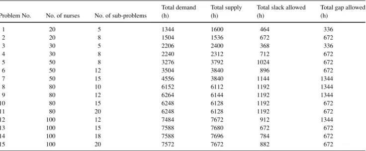
The characteristics of the data sets used in the testing are summarized in Table 1. For each instance, column 2 indicates the total number of nurses considered simultaneously. Recall that schedules are developed independently by each unit in a hospital. The total number of subproblems given in column 3 is equivalent to the total number of rotational profiles after nurse aggregation. The larger this number, the more difficult the problem is to solve. When a profile is limited to one or two shift types, as is the case here, 15 is the maximum number of subproblems that are possible without considering ratios and total working hours (5 single-shift profiles+(52) two-shift profiles). The eligible shifts for the subproblems, represented by Eqs. (4c) and (4d) were randomly generated
Table 1 Input characteristics of problem instances
Total demand Total supply Total slack allowed Total gap allowed
Problem No. No. of nurses No. of sub-problems (h) (h) (h) (h)
1 20 5 1344 1600 464 336 2 20 8 1504 1536 672 672 3 30 5 2206 2400 368 336 4 30 8 2240 2312 712 672 5 50 8 3276 3792 1024 672 6 50 12 3504 3840 896 672 7 50 15 4556 3840 1144 1344 8 80 10 6152 6112 1192 1344 9 80 12 6264 6144 1192 1344 10 80 15 6248 6128 1192 672 11 80 20 6248 6128 1192 672 12 100 12 7484 7672 912 1344 13 100 15 7588 7680 672 672 14 100 18 7588 7696 784 672 15 100 20 7572 7672 882 672
from these 15. Ratios and total hours (either 72 or 80) were then assigned. The actual data sets can be downloaded from http://www.cs.nott.ac.uk/∼tec/NRP/.
The demand, supply, allowed slack (sdt), and allowed gap
(ydt) are measured in hours and determine the tightness of
a problem’s feasible region. The total demand for all shifts over the 2-week planning horizon is given in column 4. The total supply is the sum of working hours for all nurses to be scheduled and is given in column 5. The allowed slack is the total surplus hours that can be assigned to a shift. In the demand constraint, represented by Eq. (4b), this is controlled by the upper bound on sdt, which is U Ddt−L Ddt. The
al-lowed gap is computed by summing the upper bound on the gap variables, Omax
dt , over all shifts and days, and converting
the result to hours. Depending on the problem set, a gap of either one or two nurses per shift was permitted per day. For Omax
dt =1, the total gap hours were either 336 or 672 over 14
days, depending on whether the rotational profiles included the three 8-h shift types only (24 h/day) or all five shift types (48 h/day). Those scenarios with 1344 total gap hours had Odtmax=2 and always included all five shift types (96 h/day). No problem sets had shift types other than{D, E, N}or{D, E, N, AM, PM}.
For a fixed number of profiles, the problem instances in Table 1 are generally the most difficult that we could construct. As the difference between supply and demand decreases, and as the allowed slack and allowed gap decrease, the difficulty of a problem increases. When the LP relaxation of model (1) was solved for instances with looser feasible regions, their objective function values,θLP, were almost always within a small percentage of the best IP solution found,θBEST. Hence, those results are not reported here.
6.2 Output
Table 2 summarizes the computational results. The quality of a schedule is measured by the average number of viola-tions per nurse (column 2), the total surplus hours (column 3), and the total gap hours (column 4). Under the “general results” columns, the values reported are the better of the two values obtained using the coverage ordering and the smallest number ordering schemes for constructing F . Vi-olations include the undesirable days-on and days-off pat-terns, and the number of switches in shift assignments on consecutive days. Surplus hours occur when the number of nurses assigned to a shift exceeds the demand, giving rise to idle time. Similarly, the “gap hours” indicate the total amount of undercoverage that exists in the schedule for the upcoming 2 weeks. The number of surplus and gap hours should be no greater than the maximum hours shown in the last two columns of Table 1. Because of the complementary condition sdt×ydt =0,∀d ∈D,t ∈T , it is impossible to
have a schedule in which the surplus and gap hours are both at their maximum values.
The next two columns in Table 2 give the lower bounds obtained from two different relaxations of model (1). The “LP soln” in column 5 is the objective function value found by relaxing the integrality requirements in the original model. Column 6 gives the highest value of Lagrangian objective functionθLR(μ) obtained before variable fixing was invoked at iteration 30. This is the best lower bound onθIP that was achieved using the two subgradient strategies. Of course, once variable fixing begins, this bound may and did, in fact, increase in some cases.
The last six columns in Table 2 highlight the perfor-mance of the two ordering schemes used to fix variables.