Value-at-Risk vs. Conditional Value-at-Risk in
Risk Management and Optimization
Sergey Sarykalin
Gobal Fraud Risk Management, American Express, Phoenix, Arizona 85021, [email protected]
Gaia Serraino and Stan Uryasev
Department of Industrial and Systems Engineering, Risk Management and Financial Engineering Lab, University of Florida, Gainesville, Florida 32611
{serraino@ufl.edu, uryasev@ufl.edu}
Abstract From the mathematical perspective considered in this tutorial, risk management is a procedure for shaping a risk distribution. Popular functions managing risk are value-at-risk (VaR) and conditional value-value-at-risk (CVaR). The problem of choice between VaR and CVaR, especially in financial risk management, has been quite popular in academic literature. Reasons affecting the choice between VaR and CVaR are based on the differences in mathematical properties, stability of statistical estimation, simplic-ity of optimization procedures, acceptance by regulators, etc. This tutorial presents our personal experience working with these key percentile risk measures. We try to explain strong and weak features of these risk measures and illustrate them with sev-eral examples. We demonstrate risk management/optimization case studies conducted with the Portfolio Safeguard package.
Keywords VaR; CVaR; risk measures; deviation measures; risk management; optimization; Port-folio Safeguard package
1. Introduction
Risk management is a broad concept involving various perspectives. From the mathematical perspective considered in this tutorial, risk management is a procedure for shaping a loss distribution (for instance, an investor’s risk profile). Among the vast majority of recent inno-vations, only a few have been widely accepted by practitioners, despite their active interest in this area. Conditional value-at-risk (CVaR), introduced by Rockafellar and Uryasev [19], is a popular tool for managing risk. CVaR approximately (or exactly, under certain con-ditions) equals the average of some percentage of the worst-case loss scenarios. CVaR risk measure is similar to the value-at-risk (VaR) risk measure, which is a percentile of a loss dis-tribution. VaR is heavily used in various engineering applications, including financial ones. VaR risk constraints are equivalent to the so-called chance constraints on probabilities of losses. Some risk communities prefer VaR others prefer chance (or probabilistic) functions. There is a close correspondence between CVaR and VaR: with the same confidence level, VaR is a lower bound for CVaR. Rockafellar and Uryasev [19, 20] showed that CVaR is superior to VaR in optimization applications. The problem of the choice between VaR and CVaR, especially in financial risk management, has been quite popular in academic litera-ture. Reasons affecting the choice between VaR and CVaR are based on the differences in mathematical properties, stability of statistical estimation, simplicity of optimization pro-cedures, acceptance by regulators, etc. Conclusions made from this properties may often be quite contradictive. Plenty of relevant material on this subject can be found at the website http://www.gloriamundi.org. This tutorial should not be considered as a review on VaR and
CVaR: many important findings are beyond the scope of this tutorial. Here we present only our personal experience with these key percentile risk measures and try to explain strong and weak features of these two risk measures and illustrate them with several examples. We demonstrate risk management/optimization case studies with the Portfolio Safeguard (PSG) package by American Optimal Decisions (an evaluation copy of PSG can be requested at http://www.AOrDa.com).
Key observations presented in this tutorial are as follows:
• CVaR has superior mathematical properties versus VaR. CVaR is a so-called “coherent risk measure”; for instance, the CVaR of a portfolio is a continuous and convex function with respect to positions in instruments, whereas the VaR may be even a discontinuous function.
• CVaR deviation (and mixed CVaR deviation) is a strong “competitor” to the standard deviation. Virtually everywhere the standard deviation can be replaced by a CVaR deviation. For instance, in finance, a CVaR deviation can be used in the following concepts: the Sharpe ratio, portfolio beta, one-fund theorem (i.e., optimal portfolio is a mixture of a risk-free asset and a master fund), market equilibrium with one or multiple deviation measures, and so on.
• Risk management with CVaR functions can be done quite efficiently. CVaR can be optimized and constrained with convex and linear programming methods, whereas VaR is relatively difficult to optimize (although significant progress was made in this direction; for instance, PSG can optimize VaR for quite large problems involving thousands of variables and hundreds of thousands of scenarios).
• VaR risk measure does not control scenarios exceeding VaR (for instance you can signif-icantly increase the largest loss exceeding VaR, but the VaR risk measure will not change). This property can be both good and bad, depending upon your objectives:
◦ The indifference of VaR risk measure to extreme tails may be a good property if poor models are used for building distributions. VaR disregards some part of the distribution for which only poor estimates are available. VaR estimates are statistically more stable than CVaR estimates. This actually may lead to a superior out-of-sample performance of VaR versus CVaR for some applications. For instance, for a portfolio involving instruments with strong mean reverting properties, VaR will not penalize instruments with extremely heavy losses. These instruments may perform very well at the next iteration. In statistics, it is well understood that estimators based on VaR are “robust” and may automatically disregard outliers and large losses, which may “confuse” the statistical estimation procedure.
◦ The indifference of VaR to extreme tails may be quite an undesirable property, allow-ing to take high uncontrollable risks. For instance, so-called “naked” option positions involve a very small chance of extremely high losses; these rare losses may not be picked by VaR.
• CVaR accounts for losses exceeding VaR. This property may be good or bad, depending upon your objectives:
◦ CVaR provides an adequate picture of risks reflected in extreme tails. This is a very important property if the extreme tail losses are correctly estimated.
◦ CVaR may have a relatively poor out-of-sample performance compared with VaR if tails are not modelled correctly. In this case, mixed CVaR can be a good alternative that gives different weights for different parts of the distribution (rather than penalizing only extreme tail losses).
• Deviation and risk are quite different risk management concepts. A risk measure evalu-ates outcomes versus zero, whereas a deviation measure estimevalu-ates wideness of a distribution. For instance, CVaR risk may be positive or negative, whereas CVaR deviation is always positive. Therefore, the Sharpe-like ratio (expected reward divided by risk measure) should involve CVaR deviation in the denominator rather than CVaR risk.
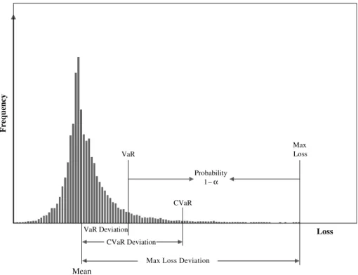
Figure 1. Risk functions: graphical representation of VaR, VaR Deviation, CVaR, CVaR Devia-tion, Max Loss, and Max Loss Deviation.
VaR, CVaR, deviations
Frequency VaR Probability 1 –α Max Loss CVaR CVaR Deviation
Max Loss Deviation
Loss
Mean
VaR Deviation
2. General Picture of VaR and CVaR
2.1. Definitions of VaR and CVaR
This section gives definitions of VaR and CVaR and discusses their use and basic properties. We refer to Figure 1 for their graphical representation.
LetXbe a random variable with the cumulative distribution functionFX(z) =P{X≤z}.
Xmay have meaning of loss or gain. In this tutorial,Xhas meaning of loss and this impacts the sign of functions in definition of VaR and CVaR.
Definition 1 (Value-at-Risk). The VaR ofX with confidence level α∈]0,1[ is VaRα(X) = min{z|FX(z)≥α}. (1) By definition, VaRα(X) is a lower α-percentile of the random variable X. Value-at-risk is commonly used in many engineering areas involving uncertainties, such as military, nuclear, material, airspace, finance, etc. For instance, finance regulations, like Basel I and Basel II, use VaR deviation measuring the width of daily loss distribution of a portfolio.
For normally distributed random variables, VaR is proportional to the standard deviation. IfX∼N(µ, σ2) andFX(z) is the cumulative distribution function ofX, then (see Rockafellar and Uryasev [19]),
VaRα(X) =FX−1(α) =µ+k(α)σ, (2) wherek(α) =√2 erf−1(2α−1) and erf(z) = (2/√π)z
0 e−t 2
dt.
The ease and intuitiveness of VaR are counterbalanced by its mathematical properties. As a function of the confidence level, for discrete distributions, VaRα(X) is a nonconvex, discontinuous function. For a discussion of numerical difficulties of VaR optimization, see, for example, Rockafellar [17] and Rockafellar and Uryasev [19].
Definition 2 (Conditional Value-at-Risk). An alternative percentile measure of risk isconditional value-at-risk(CVaR). For random variables with continuous distribution func-tions, CVaRα(X) equals the conditional expectation of X subject toX≥VaRα(X). This definition is the basis for the name of conditional at-risk. The term conditional value-at-risk was introduced by Rockafellar and Uryasev [19]. The general definition of conditional value-at-risk (CVaR) for random variables with a possibly discontinuous distribution func-tion is as follows (see Rockafellar and Uryasev [20]).
The CVaR of X with confidence level α∈]0,1[ is the mean of the generalized α-tail distribution: CVaRα(X) = ∞ −∞z dF α X(z), (3) where Fα X(z) = 0, whenz <VaRα(X), FX(z)−α 1−α , whenz≥VaRα(X).
Contrary to popular belief, in the general case, CVaRα(X) is not equal to an average of outcomes greater than VaRα(X). For general distributions, one may need to split a prob-ability atom. For example, when the distribution is modelled by scenarios, CVaR may be obtained by averaging a fractional number of scenarios. To explain this idea in more detail, we further introduce alternative definitions of CVaR. Let CVaR+α(X), called “upper CVaR,” be the conditional expectation ofX subject toX >VaRα(X):
CVaR+α(X) =E[X|X >VaRα(X)].
CVaRα(X) can be defined alternatively as the weighted average of VaRα(X) and CVaR+α(X), as follows. If FX(VaRα(X))<1, so there is a chance of a loss greater than VaRα(X), then
CVaRα(X) =λα(X)VaRα(X) + (1−λα(X))CVaR+α(X), (4) where
λα(X) =FX(VaRα(1−αX))−α, (5) whereas ifFX(VaRα(X)) = 1, so that VaRα(X) is the highest loss that can occur, then
CVaRα(x) = VaRα(x). (6) The definition of CVaR as in Equation (4) demonstrates that CVaR is not defined as a conditional expectation. The function CVaR−
α(X) =E[X |X ≥VaRα(X)], called “lower CVaR,” coincides with CVaRα(X) for continuous distributions; however, for general distri-butions it is discontinuous with respect toαand is not convex. The construction of CVaRα as a weighted average of VaRα and CVaR+α(X) is a major innovation. Neither VaR nor CVaR+
α(X) behaves well as a measure of risk for general loss distributions (both are discon-tinuous functions), but CVaR is a very attractive function. It is condiscon-tinuous with respect to
αand jointly convex in (X, α). The unusual feature in the definition of CVaR is that VaR atom can be split. If FX(x) has a vertical discontinuity gap, then there is an interval of confidence levelαhaving the same VaR. The lower and upper endpoints of that interval are
α−=F
X(VaR−α(X)) and α+=FX(VaRα(X)), whereFX(VaR−α(X)) =P{X <VaRα(X)}. WhenFX(VaR−α(X))< α < FX(VaRα(X))<1, the atom VaRα(X) having total probability
α+−α−is split by the confidence levelαin two pieces with probabilitiesα+−αandα−α−. Equation (4) highlights this splitting.
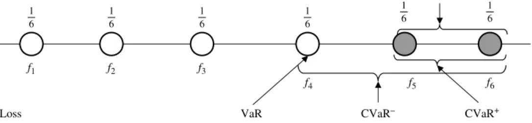
The definition of CVaR is illustrated further with the following examples. Suppose we have six equally likely scenarios with lossesf1· · ·f6. Letα=23 (see Figure 2). In this case,αdoes
Figure 2. CVaR Example 1: computation of CVaR whenαdoes not spilt the atom. CVaR 6 1 6 1 VaR Loss CVaR+ 6 1 6 1 6 1 6 1 f1 f2 f3 f4 f5 f6 CVaR–
not split any probability atom. Then VaRα(X)<CVaR−α(X)<CVaRα(X) = CVaR+α(X),
λα(X) = (FX(VaRα(X))−α)/(1−α) = 0 and CVaRα(X) = CVaR+α(X) =12f5+12f6, where f5 and f6 are losses number five and six, respectively. Now, let α=127 (see Figure 3). In this case,αdoes split the VaRα(X) atom,λα(X) = (FX(VaRα(X))−α)/(1−α)>0, and CVaRα(X) is given by
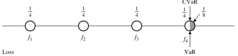
CVaRα(X) =15VaRα(X) +45CVaR+α(X) =15f4+52f5+25f6. In the last case, we consider four equally likely scenarios and α=7
8 splits the last atom (see Figure 4). Now VaRα(X) = CVaR−
α(X) = CVaRα(X), upper CVaR, CVaR+α(X) is not defined, λα(X) = (FX(VaRα(X))−α)/(1−α)>0, and CVaRα(X) = VaR(X) =f4. The PSG package defines the CVaR function for discrete distributions equivalently to (4) through the lower CVaR and upper CVaR. Suppose that VaRα(X) atom having total probability
α+−α−is split by the confidence levelαin two pieces with probabilitiesα+−αandα−α−. Then, CVaRα(X) =αα++−−αα−11−−αα−CVaR− α(X) + α−α − α+−α− 1−α+ 1−α CVaR+α(X), (7) where CVaR−
α(X) =E[X|X≥VaRα(X)], CVaR+α(X) =E[X|X >VaRα(X)]. (8) Pflug [15] followed a different approach and suggested to define CVaR via an optimization problem, which he borrowed from Rockafellar and Uryasev [19]:
CVaRα(X) = minC C+ 1 1−αE[X−C]+ , where [t]+= max{0, t}. (9) One more equivalent representation of CVaR was given by Acerbi [1], who showed that CVaR is equal to “expected shortfall” defined by
CVaRα(X) = α1 α
0 VaRβ(X)dβ.
Figure 3. CVaR Example 2: computation of CVaR whenαsplits the atom. CVaR CVaR– VaR Loss ½f5+ ½f6 = CVaR+ 6 1 6 1 6 1 6 1 6 1 6 1 121 f1 f2 f3 f4 f5 f6
Figure 4. CVaR Example 3: computation of CVaR whenαsplits the last atom. CVaR VaR Loss 4 1 4 1 8 1 4 1 4 1 f1 f2 f3 f4
For normally distributed random variables, a CVaR deviation is proportional to the standard deviation. IfX∼N(µ, σ2), then (see Rockafellar and Uryasev [19])
CVaRα(X) =E[X|X≥VaRα(X)] =µ+k1(α)σ, (10) where k1(α) = √ 2πexp(erf−1(2α−1))2(1−α)−1 and erf(z) = (2/√π)0ze−t2 dt.
2.2. Risk Measures
Axiomatic investigation of risk measures was suggested by Artzner et al. [3]. Rockafellar [17] defined a functionalR:L2→]− ∞,∞] as acoherent risk measure in the extended senseif
R1: R(C) =C for all constantC; R2: R((1−λ)X+λX )≤(1−λ)R(X) +λR(X ) forλ∈]0,1[ (convexity); R3: R(X)≤ R(X ) whenX≤X (monotonicity); R4: R(X)≤0 whenXk−X 2→0 withR(Xk)≤0 (closedness).
A functional R: L2→]−∞,∞] is called a coherent risk measure in the basic sense if it satisfies axioms R1, R2, R3, R4, and additionally the axiom
R5: R(λX) =λR(X) forλ >0 (positive homogeneity).
A functionalR: L2→]−∞,∞] is called an averse risk measure in the extended senseif it satisfies axioms R1, R2, R4, and
R6: R(X)> EX for all nonconstantX (aversity).
Aversity has the interpretation that the risk of loss in a nonconstant random variable X
cannot be acceptable; i.e.,R(X)<0, unlessEX <0.
A functional R: L2→]−∞,∞] is called an averse risk measure in the basic sense if it satisfies R1, R2, R4, R6, and also R5.
Examples of coherent measures of risk areR(X) =µX=E[X] orR(X) = supX. However,
R(X) =µ(X) +λσ(X) for someλ >0 is not a coherent measure of risk because it does not satisfy the monotonicity axiom R3.
R(X) = VaRα(X) is not a coherent nor an averse risk measure. The problem lies in the convexity axiom R2, which is equivalent to the combination of positive homogeneity and subadditivity, this last defined as R(X+X)≤ R(X) +R(X). Although positive homo-geneity is obeyed, the subadditivity is violated. It has been proved, for example, in Acerbi and Tasche [2], Pflug [15], and Rockafellar and Uryasev [20], that for any probability level
α∈]0,1[,R(X) = CVaRα(X) is a coherent measure of risk in the basic sense. CVaRα(X) is also an averse measure of risk forα∈]0,1]. An averse measure of risk might not be coherent; a coherent measure might not be averse.
2.3. Deviation Measures
In this section, we refer to Rockafellar [17] and Rockafellar et al. [24]. A functionalD:L2→ [0,∞] is called aa deviation measure in the extended senseif it satisfies
D1: D(C) = 0 for constantC, butD(X)>0 for nonconstantX;
D2: D((1−λ)X+λX)≤(1−λ)D(X) +λD(X) forλ∈]0,1[ (convexity); D3: D(X)≤dwhenXk−X
2→0 withD(Xk)≤d(closedness).
A functional is called a deviation measure in the basic sense when it satisfies axioms D1, D2, D3, and, furthermore,
D4: D(λX) =λD(X) forλ >0 (positive homogeneity).
A deviation measure in the extended or basic sense is called a coherent measure in the extended or basic sense if it additionally satisfies
D5: D(X)≤supX−E[X] for allX (upper range boundedness).
An immediate example of a deviation measure in the basic sense is the standard deviation
σ(X) = (E[X−EX]2)1/2,
which satisfies axioms D1, D2, D3, D4, but not D5. In other words, standard deviation is not a coherent deviation measure. Here are more examples of deviation measures in the basic sense:
Standard semideviations:
σ+(X) = (E[max{X−EX,0}]2)1/2, σ−(X) = (E[max{EX−X,0}]2)1/2; Mean Absolute Deviation:
MAD(X) =E[|X−EX|].
Moreover, we define theα-value-at-risk deviation measureand the α-conditional value-at-risk deviation measureas
α−VaR∆
α(X) = VaRα(X−EX) (11) and
α−CVaR∆α(X) = CVaRα(X−EX), (12) respectively. The VaR deviation measure VaR∆
α(X) is not a deviation measure in the general or basic sense because the convexity axiom D2 is not satisfied. The CVaR deviation measure CVaR∆
α(X) is a coherent deviation measure in the basic sense.
2.4. Risk Measures vs. Deviation Measures
Rockafellar et al. (originally in [24], then in [17]), obtained the following result:
Theorem 1. A one-to-one correspondence between deviation measuresDin the extended sense and averse risk measuresRin the extended sense is expressed by the relations
R(X) =D(X) +EX,
D(X) =R(X−EX); additionally,
Moreover, the positive homogeneity is preserved:
Ris positively homogeneous ↔ D is positively homogeneous.
In other words, for an averse risk measuresRin the basic sense and a deviation measures
D in the basic sense the one-to-one correspondence is valid, and, additionally, coherent R ↔coherentD.
With this theorem we obtain that for the standard deviation,σ(X), which is a deviation measure in the basic sense, the counterpart is the standard riskEX+σ(X), which is a risk averse measure in the basic sense. For CVaR deviation, CVaR∆
α(X), which is a coherent deviation measure in the basic sense, the counterpart is CVaR risk, CVaRα(X), which is a risk-averse coherent measure in the basic sense.
Another coherent deviation measure in the basic sense is the so-called Mixed Deviation CVaR, which we think is the most promising for risk management purposes. Mixed Deviation CVaR is defined as Mixed-CVaR∆ α(X) = K k=1 λkCVaR∆αk(X)
forλk≥0,Kk=1λk= 1, andαk in ]0,1[. The counterpart to the Mixed Deviation CVaR is the Mixed CVaR, which is the coherent averse risk measure in the basic sense, defined by
Mixed-CVaRα(X) = K k=1
λkCVaRαk(X).
3. VaR and CVaR in Optimization and Statistics
3.1. Equivalence of Chance and VaR Constraints
For this section, we refer to Rockafellar [18]. Several engineering applications deal with probabilistic constraints such as the reliability of a system or the system’s ability to meet demand; in portfolio management, often it is required that portfolio loss at a certain future time is, with high reliability, at most equal to a certain value. In these cases an optimization model can be set up so that constraints are required to be satisfied with some probability level rather than almost surely. Letx∈ nand letω∈Ω be a random event ranging over the set Ω of all random events. For a givenx, we may require that most of the time some random functionsfi(x, ω),i= 1, . . . , m, satisfy the inequalitiesfi(x, ω)≤0,i= 1, . . . , m; that is, we may want that
Prob{fi(x, ω)≤0} ≥pi fori= 1, . . . , m, (13) where 0≤pi≤1. Requiring this probability to be equal to 1 is the same as requiring that
fi(x, ω)≤0 almost surely. In most applications, this approach can lead to modelling and technical problems. In modelling, there is little guidance on what level ofpito set; moreover, one has to deal with the issue of constraint interactions and decide whether, for instance, it is better to require Prob{f1(x, ω)≤0} ≥p1= 0.99 and Prob{f2(x, ω)≤0} ≥p2= 0.95 or to work with a joint condition like Prob{fi(x, ω)≤0} ≥p. Dealing numerically with the functions Fi(x) = Prob{fi(x, ω)≤0} leads to the task of finding the relevant properties ofFi; a common difficulty is that the convexity offi(x, ω) with respect to xmay not carry over to the convexity of Fi(x) with respect tox.
Chance constraints and percentiles of a distribution are closely related. Let VaRα(x) be the VaRαof a loss function f(x, ω); that is,
Then, the following constraints are equivalent:
Prob{f(x, ω)≤} ≥α↔Prob{f(x, ω)> } ≤1−α↔VaRα(x)≤. (15) Generally, VaRα(x) is nonconvex with respect to x; therefore, VaRα(x) ≤ and Prob{f(x, ω)≤} ≥αmay be nonconvex constraints.
3.2. CVaR Optimization
For this section, we refer to Rockafellar and Uryasev [19] and Uryasev [29]. Nowadays, VaR has achieved the high status of being written into industry regulations (for instance, in regulations for finance companies). It is difficult to optimize VaR numerically when losses are not normally distributed. Only recently VaR optimization was included in commercial packages such as PSG. As a tool in optimization modeling, CVaR has superior properties in many respects. CVaR optimization is consistent with VaR optimization and yields the same results for normal or elliptical distributions (see definition of elliptical distribution in Embrechts et al. [6]); for models with such distributions, working with VaR, CVaR, or minimum variance (Markowitz [11]) is equivalent (see Rockafellar and Uryasev [19]). Most importantly, CVaR can be expressed by a minimization formula suggested by Rockafellar and Uryasev [19]. This formula can be incorporated into the optimization problem with respect to decision variables x∈X∈ n, which are designed to minimize risk or shape it within bounds. Significant shortcuts are thereby achieved while preserving the crucial problem features like convexity. Let us consider that a random loss functionf(x, y) depends upon the decision vector xand a random vector y of risk factors. For instance, f(x, y) =
−(y1x1+y2x2) is the negative return of a portfolio involving two instruments. Here,x1, x2 are positions andy1, y2 are rates of returns of two instruments in the portfolio. The main idea in Rockafellar and Uryasev [19] is to define a function that can be used instead of CVaR:
Fα(x, ζ) =ζ+1−1αE{[f(x, y)−ζ]+}. (16) The authors proved that
1. Fα(x, ζ) is convex with respect to (w.r.t.)α;
2. VaRα(x) is a minimum point of functionFα(x, ζ) w.r.t.ζ; 3. minimizing Fα(x, ζ) w.r.t.ζgives CVaRα(x):
CVaRα(x) = minα Fα(x, ζ). (17) In optimization problems, CVaR can enter into the objective or constraints or both. A big advantage of CVaR over VaR in that context is the preservation of convexity; i.e., iff(x, y) is convex in x, then CVaRα(x) is convex in x. Moreover, if f(x, y) is convex in x, then the function Fα(x, ζ) is convex in both xand ζ. This convexity is very valuable because minimizingFα(x, ζ) over (x, ζ)∈X× results in minimizing CVaRα(x):
min
x∈XCVaRα(x) =(x, ζmin)∈X×Fα(x, ζ). (18) In addition, if (x∗, ζ∗) minimizesF
αoverX× , then not only doesx∗minimize CVaRα(x) overX but also
CVaRα(x∗) =Fα(x∗, ζ∗).
In risk management, CVaR can be utilized to “shape” the risk in an optimization model. For that purpose, several confidence levels can be specified. Rockafellar and Uryasev [19]
showed that for any selection of confidence levelsαi and loss tolerancesωi,i= 1, . . . , l, the problem min x∈X g(x) s.t. CVaRαi(x)≤ωi, i= 1, . . . , l (19) is equivalent to the problem
min
x, ζ1,...,ζl,∈X××··· g(x)
s.t. Fαi(x, ζi)≤ωi, i= 1, . . . , l.
(20) When X and g are convex and f(x, y) is convex in x, the optimization problems (18) and (19) are ones of convex programming and, thus, especially favorable for computation. WhenY is a discrete probability space with elementsyk, k= 1, . . . , N having probabilities
pk, k= 1, . . . , N, we have Fαi(x, ζi) =ζi+ 1 1−αi N k=1 pk[f(x, yk)−ζi]+. (21) The constraint Fα(x, ζ)≤ω can be replaced by a system of inequalities by introducing additional variablesηk: ηk≥0, f(x, yk)−ζ−ηk≤0, k= 1, . . . , N, ζ+1−1α N k=1 pkηk≤ω. (22) The minimization problem in (19) can be converted into the minimization of g(x) with the constraintsFαi(x, ζi)≤ωi being replaced as presented in (22). When f is linear in x, constraints (22) are linear.
3.3. Generalized Regression Problem
In linear regression, a random variable Y is approximated in terms of random variables
X1, X2, . . . , Xn by an expression c0+c1X1+· · ·+cnXn. The coefficients are chosen by minimizing the mean square error:
min
c0,c1,...,cnE(Y −[c0+c1X1+· · ·+cnXn])
2. (23)
Mean square error minimization is equivalent to minimizing the standard deviation with the unbiasedness constraint (see, Rockafellar et al. [21, 26]):
min σ(Y −[c0+c1X1+· · ·+cnXn])
s.t. E[c0+c1X1+· · ·+cnXn] =EY. (24) Rockafellar et al. [21, 26] considered a general axiomatic setting for error measures and corresponding deviation measures. They defined an error measure as a functionalE:L2(Ω)→ [0,∞] satisfying the following axioms:
E1: E(0) = 0,E(X)>0 forX= 0,E(C)<∞for constantC; E2: E(λX) =λE(X) forλ >0 (positive homogeneity);
E3: E(X+X)≤ E(X) +E(X) for allX andX (subadditivity);
E4: {X∈ L2(Ω)| E(X)≤c} is closed for allc <∞(lower semicontinuity).
For an error measure E, the projected deviation measure D is defined by the equation
Their main finding is that the general regression problem min c0,c1,...,cnE(Y −[c0+c1X1+· · ·+cnXn]) (25) is equivalent to min c1,...,cn D(Y −[c1X1+· · ·+cnXn]) s.t. c0∈ S(Y −[c1X1+· · ·+cnXn]).
The equivalence of optimization problems (23) and (24) is a special case of this theorem. This leads to the identification of a link between statistical work on percentile regression (see Koenker and Basset [7]) and CVaR deviation measure: minimization of the Koenker and Bassett [7] error measure is equivalent to minimization of CVaR deviation. Rockafellar et al. [26] show that when the error measure is the Koenker and Basset [7] function,
Eα
KB(X) =E[max{0, X}+ (α−1−1) max{0,−X}], the projected measure of deviation is
D(X) = CVaR∆
α(X) = CVaRα(X−EX), with the corresponding averse measure of risk and associated statistic given by
R(X) = CVaRα(X), S(X) = VaRα(X). Then, min C∈(E[X−C]++ (α −1−1)E[X−C]−) = CVaR∆ α(X), arg min C∈ (E[X−C]++ (α −1−1)E[X−C]−) = VaRα(X).
A similar result is available for the “mixed Koenker and Bassett error measure” and the corresponding mixed deviation CVaR; see Rockafellar et al. [26].
3.4. Stability of Estimation
The need to estimate VaR and CVaR arises typically when we are interested in estimating tails of distributions. It is of interest, in this respect, to compare the stability of estimates of VaR and CVaR based on a finite number of observations. The common flaw in such compar-isons is that some confidence level is assumed and estimations of VaRα(X) and CVaRα(X) are compared with the common value of confidence levelα, usually, 90%, 95%, and 99%. The problem with such comparisons is that VaR and CVaR with the same confidence level mea-sure “different parts” of the distribution. In reality, for a specific distribution, the confidence levelsα1 andα2 for comparison of VaR and CVaR should be found from the equation
VaRα1(X) = CVaRα2(X). (26) For instance, in the credit risk example in Serraino et al. [27], we find that CVaR with confidence level α= 0.95 is equal to VaR with confidence level α= 0.99. The paper by Yamai and Yoshiba [30] can be considered a “good” example of a “flawed” comparison of VaR and CVaR estimates. Yamai and Yoshiba [30] examine VaR and CVaR estimations for the parametrical family of stable distributions. The authors ran 10,000 simulations of size 1,000 and compared standard deviations of VaR and CVaR estimates normalized by their mean values. Their main findings are as follows. VaR estimators are generally more stable than CVaR estimators with the same confidence level. The difference is most prominent for fat-tailed distributions and is negligible when the distributions are close to normal. A larger sample size increases the accuracy of CVaR estimation. We provide here two illustrations of Yamai and Yoshiba’s [30] results of these estimators’ performances.
In the first case, the distribution of an equity option portfolio is modelled. The portfolio consists of call options based on three stocks with joint log-normal distribution. VaR and CVaR are estimated at the 95% confidence level on 10,000 sets of Monte Carlo simulations with a sample size of 1,000. The resulting loss distribution for the portfolio of at-the-money options is quite close to normal; estimation errors of VaR and CVaR are similar. The result-ing loss distribution for the portfolio of deep out-of-the-money options is fat tailed; in this case, the CVaR estimator performed significantly worse than the VaR estimator.
In the second case, estimators are compared on the distribution of a loan portfolio, con-sisting of 1,000 loans with homogeneous default rates of 1% through 0.1%. Individual loan amounts obey the exponential distribution with an average of $100 million. Correlation coefficients between default events are homogeneous at levels 0.00, 0.03, and 0.05. Results show that estimation errors of CVaR and VaR estimators are similar when the default rate is higher; for lower default rates, the CVaR estimator gives higher errors. Also, the higher the correlation between default events, the more the loan portfolio distribution becomes fat tailed, and the higher is the error of CVaR estimator relative to VaR estimator.
As we pointed out, these numerical experiments compare VaR and CVaR with the same confidence level, and some other research needs to be done to compare stability of estimators for the same part of the distribution.
3.5. Decomposition According to Contributions of Risk Factors
This subsection discusses decomposition of VaR and CVaR risk according to risk factor contributions; see, for instance, Tasche [28] and Yamai and Yoshiba [30]. Consider a portfolio lossX, which can be decomposed as
X=n i=1
Xizi,
whereXi are losses of individual risk factors andzi are sensitivities to the risk factors, i= 1, . . . , n. The following decompositions of VaR and CVaR hold for continuous ditributions:
VaRα(X) = n i=1 ∂VaRα(X) ∂zi zi=E[Xi|X= VaRα(X)]zi, (27) CVaRα(X) =n i=1 ∂CVaRα(X) ∂zi zi=E[Xi|X≥VaRα(X)]zi. (28) When a distribution is modelled by scenarios, it is much easier to estimate quantities E[Xi|X≥VaRα(X)] in the CVaR decomposition than quantities E[Xi|X = VaRα(X)] in the VaR decomposition. Estimators of∂VaRα(X)/∂zi are less stable than estimators of
∂CVaRα(X)/∂zi.
3.6. Generalized Master-Fund Theorem and CAPM
The one-fund theorem is a fundamental result of the classical portfolio theory. It establishes that any mean-variance-efficient portfolio can be constructed as a combination of a single master-fund portfolio and a risk-free instrument. Rockafellar et al. [22] investigated in detail the consequences of substituting the standard deviation in the setting of classical theory with general deviation measures, in cases where rates of return may have discrete distributions, mixed discrete-continuous distributions (which can arise from derivatives, such as options) or continuous distributions. Their main result is that the one-fund theorem holds regardless of the particular choice of the deviation measure. The optimal risky portfolio needs not always be unique and it might not always be expressible by a master fund as traditionally conceived, even when only the standard deviation is involved. The authors introduce the
concepts of a basic fund as the portfolio providing the minimum portfolio deviation δ for a gain of exactly 1 over the risk-free rate, with the corresponding basic deviation, defined as the minimum deviation amount. Then they establish the generalized one-fund theorem, according to which for any level of risk premium ∆ over the risk-free rate, the solution of the portfolio optimization problem is given by investing an amount ∆ in the basic fund and an amount 1−∆ in the risk-free rate. In particular, the price of the basic fund can be positive, negative, or equal to zero, leading respectively to a long position, short position, or no investment in the basic fund. Rockafellar et al., first in Rockafellar et al. [23] and further in Rockafellar et al. [25], developed these concepts to obtain the generalized capital asset pricing (CAPM) relations. They find that the generalized CAPM equilibrium holds under the following assumptions: there are several groups of investors, each with utility function
Uj(ERj,Dj(Rj)) based on deviation measure Dj; the utility functions depend on mean and deviation and they are concave w.r.t. mean and deviation, increasing w.r.t. mean, and decreasing w.r.t. deviation; investors maximize their utility functions subject to the budget constraint. The main finding is that an equilibrium exists w.r.t.Di in which each group of investors has its own master fund and investors invest in the risk-free asset and their own master funds. A generalized CAPM holds and takes the form
¯ rij−r0=βij(¯rjM−r0), βij=cov(D(−Grj, rij) jM) , where ¯
rij is expected return of asseti in groupj,
r0 is risk-free rate, ¯
rjM is expected return of market fund for investor groupj,
Gj is the risk identifier for the market fundj.
From this general statement we can obtain that in classical framework when all investors are interested in standard deviation,βi is defined as
βi=cov(σ2r(ri, rM) M) .
Similarly, when all investors are interested in semideviationD(X) =σ−(X), then
βi=cov(σ2 ri, rM) −(−rM) ,
and whenD(X) = CVaR∆α(X) with continuously distributed random values, then
βi=E[ri−¯riCVaR| −rM∆≥VaRα(−rM)] α(−rM) .
It is interesting to observe in the last case that “beta” picks up only events when market is inα·100% of its highest losses; i.e.,−rM≥VaRα(−rM).
4. Comparative Analysis of VaR and CVaR
4.1. VaR Pros and Cons
4.1.1. Pros. VaR is a relatively simple risk management notion. Intuition behind
α-percentile of a distributions is easily understood and VaR has a clear interpretation: how much you may lose with certain confidence level. VaR is a single number measuring risk, defined by some specified confidence level, e.g.,α= 0.95. Two distributions can be ranked by comparing their VaRs for the same confidence level. Specifying VaR for all confidence
levels completely defines the distribution. In this sense, VaR is superior to the standard deviation. Unlike the standard deviation, VaR focuses on a specific part of the distribution specified by the confidence level. This is what is often needed, which made VaR popular in risk management, including finance, nuclear, airspace, material science, and various military applications.
One of important properties of VaR is stability of estimation procedures. Because VaR disregards the tail, it is not affected by very high tail losses, which are usually difficult to measure. VaR is estimated with parametric models; for instance, covariance VaR based on the normal distribution assumption is very well known in finance, with simulation models such as historical or Monte Carlo or by using approximations based on second-order Taylor expansion.
4.1.2. Cons. VaR does not account for properties of the distribution beyond the confi-dence level. This implies that VaRα(X) may increase dramatically with a small increase inα. To adequately estimate risk in the tail, one may need to calculate several VaRs with different confidence levels. The fact that VaR disregards the tail of the distribution may lead to unintentional bearing of high risks. In a financial setting, for instance, let us consider the strategy of “naked” shorting deep out-of-the-money options. Most of the time, this will result in receiving an option premium without any loss at expiration. However, there is a chance of a big adverse market movement leading to an extremely high loss. VaR cannot capture this risk.
Risk control using VaR may lead to undesirable results for skewed distributions. Later on we will demonstrate this phenomenon with the case study comparing risk profiles of VaR and CVaR optimization. In this case, the VaR optimal portfolio has about 20% longer tail than the CVaR optimal portfolio, as measured by the max loss of those portfolios.
VaR is a nonconvex and discontinuous function for discrete distributions. For instance, in financial setting, VaR is a nonconvex and discontinuous function w.r.t. portfolio posi-tions when returns have discrete distribuposi-tions. This makes VaR optimization a challenging computational problem. Nowadays there are codes, such as PSG, that can work with VaR functions very efficiently. PSG can optimize portfolios with a VaR performance function and also shape distributions of the portfolio with multiple VaR constraints. For instance, in port-folio optimization it is possible to maximize expected return with several VaR constraints at different confidence levels.
4.2. CVaR Pros and Cons
4.2.1. Pros. CVaR has a clear engineering interpretation. It measures outcomes that hurt the most. For example, ifL is a loss then the constraint CVaRα(L)≤L¯ ensures that the average of (1−α)% highest losses does not exceed ¯L.
Defining CVaRα(X) for all confidence levelsαin (0,1) completely specifies the distribution ofX. In this sense, it is superior to standard deviation.
Conditional value at risk has several attractive mathematical properties. CVaR is a coher-ent risk measure. CVaRα(X) is continuous with respect to α. CVaR of a convex combina-tion of random variables CVaRα(w1X1+· · ·+wnXn) is a convex function with respect to (w1, . . . , wn). In financial setting, CVaR of a portfolio is a convex function of portfolio posi-tions. CVaR optimization can be reduced to convex programming, in some cases to linear programming (i.e., for discrete distributions).
4.2.2. Cons. CVaR is more sensitive than VaR to estimation errors. If there is no good model for the tail of the distribution, CVaR value may be quite misleading; accuracy of CVaR estimation is heavily affected by accuracy of tail modelling. For instance, historical scenarios often do not provide enough information about tails; hence, we should assume a certain model for the tail to be calibrated on historical data. In the absence of a good tail model, one should not count on CVaR. In financial setting, equally weighted portfolios
may outperform CVaR-optimal portfolios out of sample when historical data have mean reverting characteristics.
4.3. What Should You Use, VaR or CVaR?
VaR and CVaR measure different parts of the distribution. Depending on what is needed, one may be preferred over the other.
Let us illustrate this topic with financial applications of VaR and CVaR and examine the question of which measure is better for portfolio optimization. A trader may prefer VaR to CVaR, because he may like high uncontrolled risks; VaR is not as restrictive as CVaR with the same confidence level. Nothing dramatic happens to a trader in case of high losses. He will not pay losses from his pocket; if fired, he may move to some other company. A company owner will probably prefer CVaR; he has to cover large losses if they occur; hence, he “really” needs to control tail events. A board of directors of a company may prefer to provide VaR-based reports to shareholders and regulators because it is less than CVaR with the same confidence level. However, CVaR may be used internally, thus creating asymmetry of information between different parties.
VaR may be better for optimizing portfolios when good models for tails are not available. VaR disregards the hardest to measure events. CVaR may not perform well out of sample when portfolio optimization is run with poorly constructed set of scenarios. Historical data may not give right predictions of future tail events because of mean-reverting characteristics of assets. High returns typically are followed by low returns; hence, CVaR based on history may be quite misleading in risk estimation.
If a good model of tail is available, then CVaR can be accurately estimated and CVaR should be used. CVaR has superior mathematical properties and can be easily handled in optimization and statistics.
When comparing stability of estimation of VaR and CVaR, appropriate confidence levels for VaR and CVaR must be chosen, avoiding comparison of VaR and CVaR for the same level ofαbecause they refer to different parts of the distribution.
5. Numerical Results
This section reports results of several case studies exemplifying how to use VaR and CVaR in optimization settings.
5.1. Portfolio Safeguard
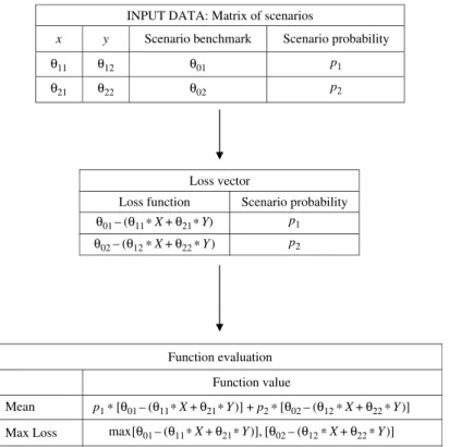
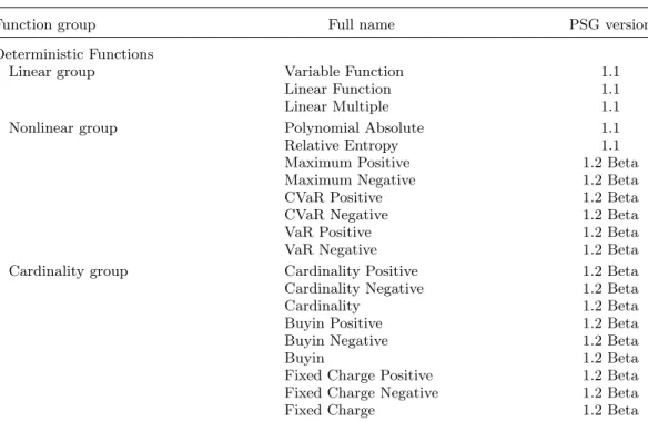
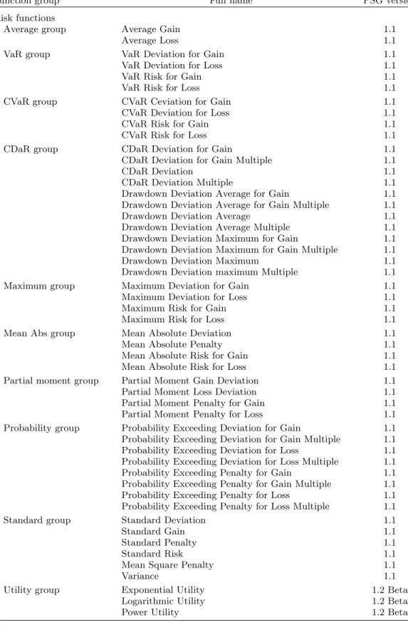
We used PSG to do the case studies. We posted MATLAB files to run these case studies in a MATLAB environment on the MathWorks website (http://www.mathworks.com), in the file exchange-optimization area. PSG is designed to solve a wide range of risk manage-ment and stochastic optimization problems. PSG has built-in algorithms for evaluating and optimizing various statistical and deterministic functions. For instance, PSG includes the statistical functions Mean, Variance, Standard Deviation, VaR, CVaR, CDaR, MAD, Max-imum Loss, Partial Moment, Probability of Exceeding a Threshold, and the deterministic functions Cardinality, Fixed Charge, and Buyin. For a complete list of functions, see Table A.1 in Appendix I. Required data inputs are matrices of Scenarios or Covariance Matrices on which statistical functions are evaluated. PSG uses a new design for defining optimiza-tion problems. A funcoptimiza-tion is defined by just providing an underlying Matrix to a Funcoptimiza-tion. Figure 5 illustrates PSG procedure for function definition (Mean and Max Loss Functions are defined: Matrix of Scenarios⇒Loss Vector⇒Functions). With PSG design all needed data, including names of variables, are taken from a Matrix of Scenarios or Covariance Matrix. PSG can calculate values and sensitivities of defined functions on decision vectors. Also, you can place functions to objective and constraint and define an optimization problem. Linear combinations of functions can be placed in the constraints. PSG includes many case
Figure 5. Example of evaluation of two PSG functions: Mean and Max Loss. INPUT DATA: Matrix of scenarios
x y Scenario benchmark Scenario probability
Loss vector
Loss function Scenario probability
Function evaluation Function value Mean Max Loss θ11 θ01 θ21 θ12 θ22 θ02 θ01– (θ11*X+θ21*Y) p1* [θ01– (θ11*X+θ21*Y)] + p2* [θ02– (θ12*X+θ22*Y)] max[θ01– (θ11*X+θ21*Y)], [θ02– (θ12*X+θ22*Y)] θ02– (θ12*X+θ22*Y) p1 p2 p1 p2
Notes. These functions are completely defined by the matrixof scenarios. Both names of variables and
function values are calculated using matrixof scenarios.
studies, most of them motivated by financial applications (such as collateralized debt obli-gation structuring, portfolio management, portfolio replication, and selection of insurance contracts) that are helpful in learning the software. To build a new optimization problems, you can simply make a copy of the case study and change input matrices and parameters. PSG can solve problems with simultaneous constraints on various risks at different time intervals (e.g., multiple constraints on standard deviation obtained by resampling, combined with VaR and drawdown constraints), thus allowing robust decision making. It has built-in efficient algorithms for solving large-scale optimization problems (up to 1,000,000 scenarios and up to 10,000 decision variables in callable MATLAB and C++ modules). PSG offers several tools for analyzing solutions, generated by optimization or through other procedures. Among these tools are sensitivities of risk measures to changes in decision variables, and the incremental impact of decision variables on risk measures and various functions of risk measures. Analysis can reveal decision variables having the biggest impact on risk and other functions, such as expected portfolio return. For visualization of these and other characteris-tics, PSG provides tools for building and plotting various characteristics combining different functions, points, and variables. It is user friendly and callable from MATLAB and C/C++ environment.
5.2. Risk Control Using VaR (PSG MATLAB Environment)
Risk control using VaR may lead to paradoxical results for skewed distributions. In this case, minimization of VaR may lead to a stretch of the tail of the distribution exceeding VaR. The purpose of VaR minimization is to reduce extreme losses. However, VaR minimization may lead to an increase in the extreme losses that we try to control. This is an undesirable feature of VaR optimization. Larsen et al. [9] showed this phenomenon on a credit portfolio with the loss distribution created with a Monte Carlo simulation of 20,000 scenarios of joint credit
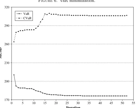
Figure 6. VaR minimization. VaR CVaR 320 290 260 230 200 170 0 5 10 15 20 25 30 35 40 45 50 55 MUSD Iteration
Notes. 99%-VaR and 99%-CVaR for algorithm A2 in Larsen et al. [9]. The algorithm lowered VaR at the
expense of an increase in CVaR.
states. The distribution is skewed with a long fat right tail. A more detailed description of this portfolio can be found in Bucay and Rosen [4] and Mausser and Rosen [13, 14]. Larsen et al. [9] suggested two heuristic algorithms for optimization of VaR. These algorithms are based on the minimization of CVaR. The minimization of VaR leads to about 16% increase of the average loss for the worst 1% scenarios, compared with the worst 1% scenarios in CVaR minimum solution. These numerical results are consistent with the theoretical results: CVaR is a coherent, whereas VaR is not a coherent, measure of risk. Figure 6 reproduces results from Larsen et al. [9] showing how iteratively VaR is decreasing and CVaR is increasing. We observed a similar performance of VaR on a small portfolio consisting of 10 bonds and modelled with 1,000 scenarios. We solved two optimization problems with PSG. In the first one, we minimized 99%-CVaR deviation of losses subject to constraints on budget and required return. In the second one, we minimized 99%-VaR deviation of losses subject to the same constraints.
Problem 1: min CVaR∆ α(x) s.t. n i=1 rixi≥r,¯ n i=1 xi= 1. (29)
Problem 2: min VaR∆α(x) s.t. n i=1 rixi≥r,¯ n i=1 xi= 1. (30)
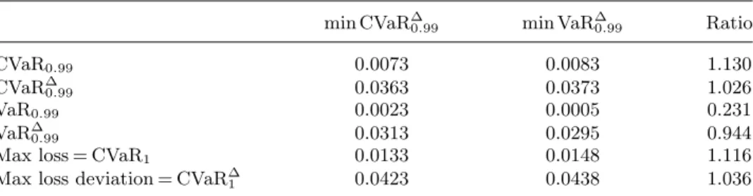
Table 1. Value of risk functions. min CVaR∆
0.99 min VaR∆0.99 Ratio
CVaR0.99 0.0073 0.0083 1.130 CVaR∆ 0.99 0.0363 0.0373 1.026 VaR0.99 0.0023 0.0005 0.231 VaR∆ 0.99 0.0313 0.0295 0.944
Max loss = CVaR1 0.0133 0.0148 1.116
Max loss deviation = CVaR∆
1 0.0423 0.0438 1.036
Notes. Column “min CVaR0.99
α ” reports the value of risk functions for the portfolio obtained by minimizing 99%-CVaR deviation, column “min VaR∆
α” reports the value of risk functions for the portfolio obtained by minimizing 99%-VaR deviation, and column “Ratio” contains the ratio of every cell of column “min VaR∆
α” to every cell of column “min CVaR∆α.”
wherexis the vector of portfolio weights, ri is the rate of return of asset i, ¯r is the lower bound on estimated portfolio return. We then evaluated different risk functions at the opti-mal points for Problems 1 and 2. Results are shown in Table 1.
Suppose that we start with the portfolio having minimal 99%-CVaR deviation. Minimiza-tion of 99%-VaR deviaMinimiza-tion leads to 13% increase in 99%-CVaR, compared with 99%-CVaR in the optimal 99%-CVaR deviation portfolio. We found that even in a problem with a rela-tively small number of scenarios, if the distribution is skewed, minimization of VaR deviation may lead to a stretch of the tail compared with the CVaR optimal portfolio. This result is quite important when we look at financial risk management regulations like Basel II that are based on minimization of VaR deviation.
5.3. Linear Regression-Hedging: VaR, CVaR, Mean Absolute, and
Standard Deviations (PSG MATLAB Environment)
This case study investigates performance of optimal hedging strategies based on different deviation measures measuring quality of hedging. The objective is to build a portfolio of financial instruments that mimics the benchmark portfolio. Weights in the replicating port-folio are chosen such that the deviation between the value of this replicating portport-folio and the value of the benchmark is minimized. Benchmark value and replicating financial instruments values are random valves. Determining the optimal hedging strategy is a linear regression problem where the response is the benchmark portfolio valve, the predictors are the repli-cating financial instrument valves, and the coefficients of the predictors to be determined are the portfolio weights. Let ˆθ be the replicating portfolio value, θ0 be the benchmark portfolio value,θ1, . . . , θI be replicating instrument values, andx1, . . . , xI be their weights. The replicating portfolio value can be expressed as follows:
ˆ
θ=x1θ1+· · ·+xIθI. (31) The coefficientsx1, . . . , xI should be chosen to minimize a replication error function depend-ing upon the residualθ0−θˆ. The intercept in this case is absent. According to the equivalence of (25) and (26), an error minimization problem is equivalent to the minimization of the appropriate deviation; see Rockafellar et al. [21] and [26]. This case study considers hedging pipeline risk in the mortgage underwriting process. Hedging instruments are 5% Mortgage-Backed Securities (MBS) forward, 5.5% MBS, and call options on 10-year treasury note futures. Changes of values of the benchmark and the hedging instruments are driven by changes in the mortgage rate. We minimize five different deviation measures: Standard Devi-ation, Mean Absolute DeviDevi-ation, CVaR DeviDevi-ation, Two-Tailed 75%-VaR, and Two-Tailed 90%-VaR. We tested in-sample and out-of-sample performance of the hedging strategies. On our set of scenarios, we found that Two-Tailed 90%-VaR has the best out-of-sample performance, whereas the standard deviation has the worst out-of-sample performance.
We think that the out-of-sample performance of hedging strategies based on different deviation measures significantly depends on the skewness of the distribution. In this case, the distribution of residuals is quite skewed.
We use here PSG definitions of Loss and Deviation functions. The Loss Function is defined as follows: Loss Function =L(x, θ) =L(x1, . . . , xI, θ0, . . . , θI) =θ0− I i=1 θixi. (32) The loss function hasjscenarios,L(x, θ1), . . . , L(x, θJ), each with probabilityp
j,j= 1, . . . , J. Here are deviation measures considered in this case study:
Mean Absolute Deviation = MAD(L(x, θ)), (33) Standard Deviation =σ(L(x, θ)), (34)
α%-VaR Deviation = VaR∆
α(L(x, θ)), (35)
α%-CVaR Deviation = CVaR∆
α(L(x, θ)), (36) Two-Tailα%-VaR Deviation = TwoTailVaR∆
α(L(x, θ))
= VaRα(L(x, θ)) + VaRα(−L(x, θ)). (37) We solved the following minimization problems:
Minimize 90%-CVaR Deviation min
x CVaR ∆
0.9(L(x, θ)) (38)
Minimize Mean Absolute Deviation min
x MAD(L(X, θ)) (39)
Minimize Standard Deviation
min
x σ(L(x, θ)) (40)
Minimize Two-Tail 75%-VaR Deviation min
x TwoTailVaR ∆
0.75(L(X, θ)) (41)
Minimize Two-Tail 90%-VaR Deviation min
x TwoTailVaR ∆
0.9(L(X, θ)). (42)
The data set for the case study includes 1,000 scenarios of value changes for each hedging instrument and for the benchmark. For the out-of-sample testing, we partitioned the 1,000 scenarios into 10 groups with 100 scenarios in each group. Each time, we selected one group for the out-of-sample test and we calculated optimal hedging positions based on the remain-ing nine groups containremain-ing 900 scenarios. For each group of 100 scenarios, we calculated the ex ante losses (i.e., underperformances of hedging portfolio versus target) with the optimal hedging positions obtained from 900 scenarios. We repeated the procedure 10 times, once for every out-of-sample group with 100 scenarios. To estimate the out-of-sample perfor-mance, we aggregated the out-of-sample losses from the 10 runs and obtained a combined set including 1,000 out-of-sample losses. Then, we calculated five deviation measures on the out-of-sample 1,000 losses: Standard Deviation, Mean Absolute Deviation, CVaR Deviation, Two-Tail 75%-VaR Deviation, and Two-Tail 90%-VaR Deviation. In addition, we calculated three downside risk measures: 90%-CVaR, 90%-VaR, and Max Loss = 100%-CVaR on the out-of-sample losses. Tables 2 and 3 show the results.
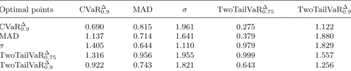
By minimizing the Two-Tail 90%-VaR Deviation, we obtained the best values for all three considered downside risk measures (negative loss indicates gain). Minimization of CVaR deviation lead to good results, whereas minimization of standard deviation gave the worst level for three downside risk measures.
Table 2. Out-of-sample performance of various deviations on optimal hedging portfolios. Optimal points CVaR∆
0.9 MAD σ TwoTailVaR∆0.75 TwoTailVaR∆0.9
CVaR∆ 0.9 0.690 0.815 1.961 0.275 1.122 MAD 1.137 0.714 1.641 0.379 1.880 σ 1.405 0.644 1.110 0.979 1.829 TwoTailVaR∆ 0.75 1.316 0.956 1.955 0.999 1.557 TwoTailVaR∆ 0.9 0.922 0.743 1.821 0.643 1.256
Notes. Each row reports values of five different deviation measures evaluated at optimal hedging points
obtained with five hedging strategies.
5.4. Example of Equivalence of Chance and VaR Constraints
(PSG MATLAB Environment)
This case study illustrates the equivalence between chance constraints and VaR constraints, as explained in§3.1. We will illustrate numerically the equivalence
Prob{L(x, θ)> } ≤1−α↔VaRα(L(x, θ))≤, (43) where Loss FunctionL(x, θ) =L(x1, . . . , xI, θ1, . . . , θI) =− I i=1 θixi. (44)
The case study is based on a data set including 1,000 return scenarios for 10 clusters of loans. Here, I= 10 is the number of instruments, θ1, . . . , θI are rates of returns of instruments,
x1, . . . , xI are instrument weights, and L(x, θ) is a portfolio loss. We solved two portfolio optimization problems. In both cases we maximized the estimated return of the portfolio. In the first problem, we imposed a constraint on probability; in the second problem, we imposed an equivalent constraint on VaR. In particular, in the first problem we require the 95%-VaR of the optimal portfolio to be at most equal to the constant, whereas in the second problem we require the probability of losses greater thanto be lower than 1−α= 1−0.95 = 0.05. We expected to obtain at optimality the same objective function value and similar optimal portfolios for the two problems. Problem formulations are as follows:
Problem 1: max E[−L(x, θ)] s.t. Prob{L(x, θ)> } ≤1−α= 0.05, vi≤xi≤ui, i= 1, . . . , I, I i=1 xi= 1. (45)
Table 3. Out-of-sample performance of various downside risks on optimal hedging portfolios.
Optimal points Max Loss CVaR0.9 VaR0.9
CVaR∆ 0.9 −18.01 −18.05 −18.08 MAD −16.49 −17.44 −17.88 σ −13.31 −15.29 −15.60 TwoTailVaR∆ 0.75 −15.31 −16.19 −16.71 TwoTailVaR∆ 0.9 −18.02 −18.51 −18.66
Notes. Each row reports values of three different risk measures evaluated at optimal hedging points obtained
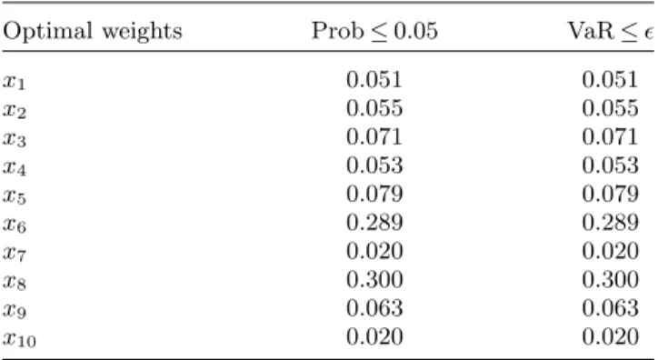
Table 4. Chance vs. VaR constraints.
Optimal weights Prob≤0.05 VaR≤
x1 0.051 0.051 x2 0.055 0.055 x3 0.071 0.071 x4 0.053 0.053 x5 0.079 0.079 x6 0.289 0.289 x7 0.020 0.020 x8 0.300 0.300 x9 0.063 0.063 x10 0.020 0.020
Notes. Optimal portfolios obtained on the same data set when we
maximized return with the chance constraint (the first column) and with the VaR constraint (the second column).
Problem 2: max E[−L(x, θ)] s.t. VaRα(L(x, θ))≤, vi≤xi≤ui, i= 1, . . . , I, I i=1 xi= 1. (46)
In the problems, vi is the lower bound on position for asseti, and ui is the upper bound on position for asset i. We also have the budget constraint: sum of weights is equal to 1. The two problems at optimality selected the same portfolios and have the same objective function value of 120.19. Table 4 shows the optimal points.
5.5. Portfolio Rebalancing Strategies: Risk vs. Deviation
(PSG MATLAB Environment)
In this case study we consider a portfolio rebalancing problem. A portfolio manager allocates his wealth to different funds periodically solving an optimization problem and in each time period building the portfolio that minimizes a certain risk function, given budget constraints and bounds on each exposure. We solved the following problem:
min R(x, θ)−k∗E[−L(x, θ)] (47) s.t. I i=1 xi= 1 (48) vi≤(xi)≤ui i= 1. . . , I, (49) where we denote by R(x, θ) a risk function, E[−L(x, θ)] is the expected portfolio return,
θ1, . . . , θI are rates of returns of instruments, and x1, . . . , xI are instrument weights. The scenario data set is composed of 46 monthly return observations for seven managed funds; we solved the first optimization problem using the first 10 scenarios, then we rebalanced the portfolio monthly. We used as risk functions VaR, CVaR, VaR Deviation, CVaR Deviation, and Standard Deviation.
We then evaluated Sharpe ratio and mean value of each sequence of portfolios obtained by succesively solving the optimization problem with a given objective function. Results are reported in Tables 5 and 6 for different values of the parameterk. Both in terms of Sharpe ratio and mean portfolio value we found a good performance of VaR and VaR deviation
Table 5. Out-of-sample Sharpe ratio.
k VaR CVaR VaR Deviation CVaR Deviation Standard Deviation
−1 1.2710 1.2609 1.2588 1.2693 1.2380
−3 1.2711 1.2667 1.2762 1.2652 1.2672
−5 1.2712 1.2666 1.2721 1.2743 1.2628
Notes. Sharpe ratio for the rebalancing strategy when different risk functions are used in the
objective function with several values of parameterk.
Table 6. Out-of-sample portfolio mean return.
k VaR CVaR VaR Deviation CVaR Deviation Standard Deviation
−1 0.2508 0.2556 0.2445 0.2567 0.2425
−3 0.2645 0.2575 0.2631 0.2598 0.2576
−5 0.2663 0.2612 0.2662 0.2617 0.2532
Notes. Portfolio mean return for the rebalancing strategy when different risk functions are used
in the objective function with several values of parameterk.
minimization, whereas standard deviation minimization gives inferior results. Overall, we rebalanced the portfolios 37 times for each objective function. Results depend on the scenario data set and on the parameterk; thus, we cannot conclude that minimization of a certain risk function is always the best choice. However, we observe that in the presence of mean reversion, the tails of historical distribution are not good predictors of the tails in the future. In this case, VaR disregarding the tails may lead to a good out-of-sample portfolio performance. In fact, VaR disregards the unstable part of the distribution.
Appendix I
Table A.1. PSG functions.
Function group Full name PSG version
Deterministic Functions
Linear group Variable Function 1.1
Linear Function 1.1
Linear Multiple 1.1
Nonlinear group Polynomial Absolute 1.1
Relative Entropy 1.1
Maximum Positive 1.2Beta
Maximum Negative 1.2Beta
CVaR Positive 1.2Beta
CVaR Negative 1.2Beta
VaR Positive 1.2Beta
VaR Negative 1.2Beta
Cardinality group Cardinality Positive 1.2Beta
Cardinality Negative 1.2Beta
Cardinality 1.2Beta
Buyin Positive 1.2Beta
Buyin Negative 1.2Beta
Buyin 1.2Beta
Fixed Charge Positive 1.2Beta
Fixed Charge Negative 1.2Beta