PRELIMINARY
H
AIRCUTS
Federico Sturzenegger and Jeromin Zettelmeyer1
First Draft, May 30, 2004 This Draft: October, 2004
Abstract
This paper estimates “haircuts”—realized investor losses—in recent debt restructurings in Russia, Ukraine, Pakistan, Ecuador, Argentina, and Uruguay. Haircuts are computed as the percentage difference between the present values of old and new instruments, discounted at the yield prevailing immediately after the exchange. We find substantial differences between average haircuts ranging from 10-15 percent (Uruguay) to more than 70% in the case of the Argentina domestic exchanges. Some (but not all) exchanges exhibit substantial variations in haircuts even within the exchange, depending on the instrument tendered. Thus, “intercreditor equity” was often violated ex post, at least in a present value sense. When domestic and foreign residents could be identified we find that exchanges have tended to be milder on domestic bondholders.
1
Universidad Torcuato di Tella and International Monetary Fund, respectively; [email protected];
[email protected]. We are very grateful to Eduardo Borensztein, Harald Finger, Olivier Jeanne, Eduardo Levy-Yeyati, Simon Johnson, Jens Nysted and Ernesto Schargrodsky, for comments and for sharing data, and to Francisco Ceballos, Luciana Esquerro, Priyanka Malhotra, Luciana Monteverde and Sofia Zerbarini, for outstanding research assistance. This paper should not be reported as representing the views of the IMF. The views expressed are those of the authors and do not necessarily reflect the views of the IMF or IMF policy.
I. INTRODUCTION
This paper estimates investor losses—or “haircuts,” in market parlance—associated with the new generation of sovereign debt restructurings that started with Russia’s 1998 default and has since extended to a number of emerging market countries in Eastern European, the Middle East, and Latin America. Specifically, we examine the December 1999 exchange of Pakistani Eurobonds, the 1999 “Novation” exchange of Russian domestic debt, a string of restructurings in Ukraine during 1998 and 1999, the 2000 external debt exchanges in Russia, Ukraine and Ecuador, the November 2001 “Phase 1” exchange of Argentine bonds, the 2002 “Pesification” of Argentine debt, and the May 2003 Uruguayan bond exchange.
One motivation for the empirical exercise conducted in this paper is simply to better understand emerging market debt as an asset class. A key question in this regard is how much investors typically recover in a default situation, and whether there are substantial variations from one debt restructuring to another. It is also interesting whether investors were treated equally within each debt restructuring, or whether some instrument holders came out better than others, and if so, whether there is a systematic relationship with the characteristics of the initial instrument or the residence of the bondholder.
A second motivation is related to economic policy. Some of the debt restructurings that we consider in this paper, such as Pakistan’s 1999 Eurobond restructuring, were based on a deliberate decision by official creditors to force private creditors to take some losses in order to reduce the moral hazard associated with official debt forgiveness. The question is whether they succeeded, and how big those losses turned out to be ex post. However, policy makers in international institutions and creditor countries are also interested in the continued existence of a sovereign debt market, and concerned about debtor moral hazard. In particular, they would like distressed debtors to “act in good faith” in restructuring their debts, avoiding restructuring proposals that fall below commonly accepted standards of what defines a reasonable offer. But what is normal or reasonable in this context? To answer this question, it is necessary to know something about the magnitude of investor losses in past restructurings. Though this is the first paper, to our knowledge, to systematically compute “haircuts” for a range of debt restructurings with a common methodology, there has been important related work. First, there is a literature on “private sector involvement” in the recent debt crises, including Eichengreen and Rühl (2000), Lipworth and Nystedt (2001), IMF (2001), World Bank (2002), and Cline (2004) that discusses the terms of recent debt restructurings and describes reductions in face value as well as the market performance of bonds before and after specific events. Unlike this study, however, these papers do not estimate net present value losses suffered by investors. Second, there are some papers on average returns to emerging market debt, most recently Klingen, Weder and Zettelmeyer (2004), who estimate returns to emerging market debt since 1970 and for shorter subperiods for a variety of emerging market countries. However, their sample ends in 2000 and excludes the transition economies; thus, they miss most of the debt crises studied in this paper. Moreover, their results are based on annual data, which does not allow the computation of losses associated
- 3 -
with specific debt restructuring events. Third, investment banks and creditor organizations, as well as the International Monetary Fund, have in some cases estimated the “haircuts” associated with some specific crises. However, these estimates are generally not published, the computations underlying them are often not transparent, and the methodologies used may vary across episodes.2
The methodology adopted in this paper is to compute investor losses in this paper as the difference between the net present value of the original and the new (restructured) instruments, using the immediate post-exchange (“exit”) yield of the new instrument to discount both payments streams. Thus, these are the realized, ex post losses of investors in the immediate aftermath of a restructuring. In the section that follows, we justify this measure of investor losses in some detail.
Our main results are as follows. First, there are substantial differences between the average haircuts in the exchanges, ranging from haircuts in the order of 10 percent to more than 70 percent. Second, some (but not all) exchanges exhibit substantial variations in the haircut even within the same exchange, depending on the instrument tendered. Thus, in most cases, “intercreditor equity” was violated ex post, at least in a present value sense. Finally, we find that when it was possible to distinguish between local and foreign bondholders, the former were usually offered more favorable terms. We explore some regularities in within-exchange variations in investor losses, and some conjectures of what might be driving them.
II. MEASURING INVESTOR LOSSES
Economists and market participants would generally agree that the losses suffered by investors in a debt exchange should be measured by comparing the net present value of cash flows promised under the old and new debt instruments. The question is whether these cash flows should be discounted using a common interest rate or different interest rates, and what discount rates should be used.
For example, an investor holding an instrument since the time of its emission or purchase may feel that he loses to the extent that the market value of the new debt instrument is lower than the market value of the old instrument at the time of its purchase; in effect comparing the NPV of the original instrument discounted with pre-crisis yields to the NPV of the new instrument discounted with the “exit yield” prevailing after the exchange. For our purposes, however, this definition of investor losses is too broad, since it includes any loss attributable to the deterioration of economic fundamentals prior to the crisis, rather than the loss attributable to the terms of the exchange. At the other extreme, it is unhelpful to compare the market value of the old instrument just prior to the exchange with the market value of the new instrument just after the exchange, since, in a world of perfect foresight, these should be
2
For an exception, see the IMF’s published report on the Uruguay debt exchange; this includes some estimates of NPV losses for investors (IMF, 2003, Appendix II, p. 49).
equal. Any measured gain or loss will thus reflect the extent to which the result of the exchange was incorrectly anticipated, independently of the terms of the exchange.
Like most authors, we thus take the view that the cash flows promised under the new and old instruments must be compared using the same discount rate (except for adjustments reflecting differences in maturities, as explained below). From the perspective of measuring
realized losses the appropriate discount rate is the yield implicit in the market value of the new instrument immediately after the close of the exchange: this will reflect the results of the exchange (i.e., the participation rate) but not news about economic fundamentals that becomes available after the exchange, i.e. after the results of the exchange are known. Thus, our approach is to compare the market value of the new instruments, plus any cash payment received, with the NPV of the payments remaining on the old instruments, discounted using the yield of the new instruments (r):
( , ) ( , )
H ≡NPV old r −NPV new r . (1)
One nice property of a haircut in this particular definition is as a measure of the “coercion”, or pressure, that must have been exerted on investors in order to solve the free rider problem associated with a particular exchange. To see this, let i( |
{ }
j )j i u accept a
≠ denote the expected
payoff from accepting the exchange offer, conditioning on the actions of other investors (i.e. accept or reject), and i( |
{ }
j )j i
u reject a ≠ the expected payoff from holding on to the old debt instrument. To the extent that the exchange was successful, it must have been true that for the investors that accepted the exchange offer,
{ }
{ }
( | ) ( | ) 0 i j j i i j j i u accept a ≠ −u reject a ≠ ≥ , (2){ }
( | ) i j j i u accept a≠ is just the market value of the new instrument, that is, the price that can
be observed in the secondary market after the exchange. By definition this is equal to the net present value of the cash flow promised by the new instrument, discounted by the secondary market yield of these new instruments. Thus, i( |
{ }
j ) ( , )j i
u accept a ≠ =NPV new r . Using (1)
and (2), one obtains:
{ }
( , ) i( | j ) j i H NPV old r u reject a ≠ ≤ − , (3){ }
( | ) i j j iu reject a ≠ is the (unobservable) utility, or value, of holding on to the old instrument, conditioning on the outcome of the exchange, given expectations about what would happen to old instruments that were not traded in. NPV old r( , ) is the net present value of the cash flow associated with the old instrument discounted at the yield of the new instrument—that
- 5 -
is, assuming “equal treatment”, or no discrimination. In actual fact, of course, there was discrimination, in the sense of an open or implicit threat that the old instruments would not be serviced in the same way as the new ones, so ( , ) i( |
{ }
j )j i
NPV old r u reject a
≠
− was
typically greater than zero. The haircut, H, tells us how big the difference between the theoretical value of the old instrument, NPV old r( , ), and its value as it was actually perceived must have been, at a minimum, to make the exchange work (in the sense that equation (2) was satisfied), given the quality of the exchange offer NPV new r( , ). In this sense, H measures the (minimum) “coerciveness” of an exchange.
While conceptually simple, measuring H as defined in (1) involves a number of practical complications. The most important of these is that the maturities of the new and old instruments will typically not be the same. Suppose, as will generally be the case, that the maturity of the new instrument is longer than that of the old instrument, and that the term structure is upward sloping. Then the yield of this new instrument will be higher than that of a new instrument with the length of the old instrument. By discounting the old instrument with this higher yield, we will tend to underestimate the NPV that we would have obtained by discounting with a yield corresponding to the maturity of the old instruments, and consequently the extent of the haircut.
To deal with this problem, we attempt to estimate the “new” yield corresponding to the average length of the old instrument by interpolating the yields on new instruments (there are usually more than one) accordingly. When this is not possible—as it may be if all new instruments are longer than the old one in terms of remaining maturity— [or when the yield curve does not have any discernible pattern] we use the yield on the new instrument that is closest to the old bond in terms of average length, and make an adjustment using the yield curve on US treasury bills.
A second complication is that by applying the new instrument yield to the old instrument we are also assuming that both instruments were of the same seniority. However, in some cases—for example the Russian exchange in which new instruments were upgraded to debt of the Russian Federation as opposed to debt owed by a state-owned bank—the sovereign resorted to security enhancements to make new instruments more attractive. By discounting the old instrument’s cash flow with the yield of the new instruments we would be incorrectly applying this enhancement to the old instrument. In this case, we may be overestimating the haircut with respect to the true old instruments.
A third complication relates to the treatment of unpaid interest. We treat unpaid interest on the old bonds as part of the outstanding claim, but generally ignore interest on interest. The main exception is the Russian exchange, in which cash payments associated with past due interest were spread out over a long time period; in this case, we compute the value of PDI as a net present value.
A fourth complication arises when the exchange involves a change in the currency of denomination of the two instruments. In this case old and new instruments cannot be
discounted at the same rate. Fortunately, in most cases there are both foreign and domestic currency exit yields, so it just a matter of applying the discount factor of the relevant currency in each case, adjusted by maturity when necessary.
A fifth complication arises from the lack of information. In several instances the package received by the bondholders contained a combination of new bonds, but there is little precision as to how much bond of each was exchanged for each particular instrument. In general, when facing such lack of information we compute two bounds. In one the bondholder receives the best possible instrument. In the other, she receives the worst. In general (but not always), these alternatives do not generate substantially different results. Finally, in some instances—the Ukraine exchanges in 1998 and the November 2001 Argentine exchange—the new instrument was not immediately traded, and thus there is no “exit yield” for these bonds. In the case of Ukraine we obtain exit yields from the market returns on similar instruments issued immediately after the exchange. In the case of Argentina, old bonds continued to be traded after the exchange, and the new instruments were eventually traded, albeit after a substantial time lag. As explained in more detail below, the implicit yields of these two groups of bonds are used to compute upper and lower bound estimates for the true haircut. Fortunately, they are sufficiently close to be informative. Given the complexities of the computation it is not surprising that this exercise has not been tackled yet. We believe that the contribution of this paper lies in resolving these complexities in a consistent fashion and obtaining comparable numbers among the different exchanges.
III. RESULTS
A. Russia3
Russia’s devaluation on August 18, 1998 led to a default on its domestically issued debt, while the government tried to stay current on its external obligations. On August 25 the government made a first restructuring offer on its Ruble denominated “GKO” treasury bills, which was rejected by market participants. In March of 1999, the government finalized a restructuring agreement, known as “novation”, with holders of GKOs and longer term Ruble denominated OFZs, which had rejected the government’s August 1998 exchange offer. Under the novation scheme, holders of GKO or OFZs would accept to have their scheduled payment discounted to August 19, 1998, at a rate of 50 percent per annum. Subsequently, they would received a package including a combination of cash and very short term instruments in addition to longer term OFZs. The short term component included a cash payment equivalent to 3.33% of the adjusted nominal value, 3.33% in 3-month GKOs (these
3 This material has in part been reconstructed with information from NUPI, Center for Russian Studies. For a
complete review of the events leading to the Russian crisis see Kharas et al (2001), and for a comprehensive description of the Russian debt restructuring is provided by Santos (2003). See also JP Morgan (1997, 2000).
- 7 -
bonds had an issue date of December 15 so that they would expire shortly after the exchange on the 24th of March), 3.33% in a 6-month GKOs (also with an issue date on December 15), and “cash value” OFZ for 20 percent of nominal value that could be used at par to pay tax obligations that were in arrears as of July 1st, 1998, or to purchase newly issued shares of Russian banks. The remaining 70% was returned in OFZs with maturities ranging from 4 to 5 years with coupons of 30, 25, 20, 15 and 10 each year, respectively. With the exception of cash, any receipts from selling these OFZs had to be deposited in restricted ruble accounts that could be used to purchase selected Russian corporate bonds and equity securities.4
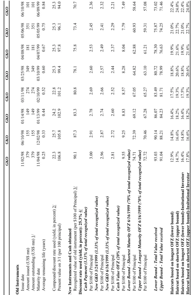
Table 1 shows the results for the GKO exchange. For brevity we only show the first GKO maturing in each of the months for which there were GKO instruments restructured.5 The upper half of the table shows the present value at the time of the exchange of GKOs with a face value of 100 rubles. The exit yield on GKOs was used to discount GKOs payments maturing after March 1999 to the time of the exchange. The average ruble deposit rate in the Russian financial sector was used to bring payments due prior to the exchange date to March 1999.6
The lower half of the table shows what investors received in return, both in “cash items” and in longer term OFZs with all flows discounted at 25.3%, the average yield of GKOs during March 1999. Recall that the values are computed taking into account that the original flow had been discounted at a 50% nominal interest rate back to August (line “recognized value of old instrument”). Thus, if an instrument had a face value recognition of 90% (see first column) the 3.33% of cash implies a payment of 3.33*0.9=3 per 100 of face value, and so on with the other instruments.
As there is little information as to the exact number of OFZs given to each GKO holder, we compute two bounds. One (lower) bound considers that the holder received only the shorter of the OFZs, thus providing the most convenient alternative to bond holders. The other (upper) bound considers that the bond holders only obtained the longest version. Fortunately, the difference between the two bounds is minimal so the computation is meaningful.
4 Nonresidents electing to convert and repatriate restricted rubles had available an alternative but it entailed
additional losses.
5 The complete table for all GKOs bonds identified by Bloomberg as defaulted can be found in
www.utdt.edu/~fsturzen.
6 Both rates were obtained from the Rusian Central Bank, at www.cbr.ru/eng/statistics/. This page provide
Finally, the haircuts are computed, in percentage terms, by subtracting the total value obtained from the present value of the old claim and dividing by the latter. The numbers indicate that investors lost between 13% and 24% of the pre-existing claim.78
Russian institutional holders, which were required to hold GKO/OFZs by law, received slightly different terms (10 percent cash, 10 percent in 3 month GKOs, 10 percent in 6 month GKOs, 20 percent in cash value OFZs and 50 percent in OFZs with maturities ranging from 4 to 5 years).9 While the larger share of cash payments may seem to indicate a better deal, the fact that the coupon rate offered on OFZs was larger than the market discount rate, implies that the PV of the new claims decreased when the cash items increased. The final two lines of Table 1 show the corresponding haircuts. The differences with the previous case, are, in any case, very small.
The banking crisis that followed the devaluation-default decision eventually had implications for Russian external debt payments. On December 2 of 1998, the state-owned Vneshekonombank missed a 362 million payment on its “PRINs”, and on June 2, 1999, it missed a payment on its “IANs”. “PRINs” and “IANs” were dollar denominated, floating interest, long term bonds with total face value of US$ 29 billion that had been issued in 1997 following an agreement with the London Club to restructure Soviet era debt owed to Western commercial banks. Though widely considered as part of Russia’s external public debt, they were technically obligations of Vneshekonombank rather than obligations of the Russian Federation. In addition, Russia had issued several Eurobonds between 1996 and 1998, on which it did not default.
In May 1999, the Russian government also defaulted on Soviet era MinFin 3. However, in January 2000 it offered to exchange the bonds for one of two alternatives. Either a new eight-year bond similar to the original instrument, i.e. in US dollars and with a coupon of 3%, or a four year OFZ (ruble denominated bond) paying an interest rate of 15% for the first year and 10% thereafter, with interest paid semiannually and bullet principal payment. Table 2 shows the haircuts involved in the MinFin 3 restructuring. Grossing up the missed principal payment by the US treasury bill,10 was worth 106.2 on February 2nd of 2000. The new
7 It is plausible but wrong to think that the low haircut is the result that the computation is done in rubles,
unattentive to the fact that the exchange rate was devaluing very quickly. At the time of the exchange, expected depreciation of the local currency is embedded in the interest rates, if this expectation is very high so will interest rates, and therefore higher will be the PV loss from maturity extensions and low interest rates.
8 It may be worth noticing that we are ignoring the restrictions imposed by the fact that amounts had to be
placed in restricted rouble accounts. Thus these haircut computations correspond to those faced by an investor that would not exit the Russian market immediately.
9 Some investors that refused to take the “novation” offer were paid according to the original (ruble) terms;
however, non-residents were not allowed to repatriate their funds for a period of 5 years.
10 This is equivalent to assuming that the bondholders had taken their money out of Russia and into a safe
- 9 -
year bond, discounted at the exit yield of the new bond of 17.5%,11 delivers a PV of 45.6 implying a haircut of 57%. The OFZ alternative, discounted at the only slightly higher ruble rate of 20% gives a PV of 76 and a haircut of only 28.3%. While the haircut computation delivers a smaller value for the conversion to a ruble instrument, it is reported (and this is confirmed by the amounts issued) that most investors opted for the first alternative.12
Shortly after the MinFin3 restructuring proposal, on February 11, 2000 Russia offered to exchange both Vnesh’s PRINs and IANs for two new Eurobonds of the Russian Federation. The deal was closed in August 2000, restructuring all PRINs and IANs with a total of 21 billion of new instruments issued in exchange for an original nominal value of 31.8 billion (the original face value of $29 billion, plus past due interest amounting to US$ 2.8 billion). In exchange for IANs, PRINs, bondholders were offered a 2030 Eurobond with a step up (2.25 to 7.5 percent) coupon, after a face value reduction of 37.5 percent for the longer maturity PRINs and 33 percent for the shorter maturity IANs. Past due interest was compensated (without face value reduction) by a 2010 Eurobond with a fixed 8.25 percent coupon, and a small cash “sweetener”.
Table 3 summarizes the Russian PRIN,and IAN exchange. The upper half of the table shows the terms and present values of 100 units of PRINs and IANs, respectively, at the time of the exchange,13 as well as the associated past due interest accumulated between December of 1998 and February of 2000. As explained in the last section, the present values are computed using the yield curve of Russian debt adjusted for the shorter maturities of the PRINs and IANs. The adjustment is easy in this case since a range of undefaulted Russian Eurobonds were trading in the secondary markets at the time, whose yields can be used to interpolate. Since the Russian Eurobond yield curve was quite flat, it makes very little difference.
11 Corresponding to its first day of trading, the 29th of June of 2000.
12 A possible may be found in that while the bonds that replaced the MinFin 3 were issued February 1st 2000,
the option to exchange the MinFin 3 was open ended. Thus for bond holders trading in later than this date the haircut computation may be slightly different. By year end most bondholders had traded in their original holdings.
13 For most instruments that are examined in this paper, if an investor had bought and held 100 units of principal
since the time of issue, the face value of his or her claim at the time of the debt exchange would also be 100 units. However, there are two exceptions: first, amortizing bonds, that were in part repaid before the debt exchange, and bonds with capitalized interest payments, whose face value increased before the debt exchange. In these cases, the computations in the tables (PVs of the old instruments values obtained in the form of new
instruments) refer to 100 units of principal at the time of the exchange, rather than at the time of issue. For
example, the interest paid on Russian PRINs prior to the December 1998 default was in part capitalized into IANs, so that an investor owning 100 PRINs at the time of issue would have owned a basket of 100 PRINs and about 3.6 IANs at the time of the debt exchange. However, the computations in the left column of table 1 refer
The lower half of the table shows what investors received in return: a small cash payment for PDI, some amount of the 2010 Eurobond for PDI, and the 2030 Eurobond in exchange for the original instrument, after a face value reduction. The lines “value obtained (per 100 units of principal)” are computed by subtracting the corresponding face value reduction (if any) from 100 units of the old bond and then multiplying with the price of one new bond. For example, in the “PRINs” column, (100 – 37.5)*0.418 = 26.1. Finally, the haircuts are computed, in percentage terms, by subtracting the total value obtained from the present value of the old claim (including PDI) and dividing by the latter. The main result is that investors lost about 50 percent of the pre-exchange claim. Percentage losses on the shorter IANs were very slightly higher than on the longer PRINs.
P R E L IM INAR Y GK O G K O GKO GK O G K O GK O GKO GK O O ld In st ru m ent s Is su e d at e 11/ 02/ 98 06 /1 0/ 98 01 /1 4/ 98 03 /1 1/ 98 03/ 25/ 98 04 /0 8/ 98 05 /0 6/ 98 06/ 10 /9 8 A m ou nt is su ed ( U S$ m n) 379 15 5 149 27 4 349 18 1 351 10 1 A m ount o ut st and ing (U S$ m n) 1 / 37 9 155 149 27 4 349 18 1 351 10 1 M at uri ty da te 11/ 04/ 98 12 /0 2/ 98 01 /1 3/ 99 02 /1 0/ 99 03/ 10/ 99 04 /0 7/ 99 05 /0 5/ 99 06/ 09 /9 9 A ve ra ge r em ai ni ng li fe ( ye ar s) 0. 25 0. 33 0.44 0.5 2 0. 60 0. 67 0.75 0.8 4 C om po un d/d is co un t rate u sed ( yield , in p er cen t) 2 / 22 .3 25 .7 24.2 22. 8 25 .3 25.3 25.3 25. 3 P re se nt v al ue on 3 /1 ( pe r 10 0 pr in ci pa l) 106 .8 10 5.8 102.9 101. 2 99 .4 97.8 96.1 94. 0 N ew In st ru m en ts a nd Ca sh o b ta in ed R eco gn ized v alu e o f o ld in st ru m en t (p er $ 10 0 o f Prin cip al) 3 / 90 .1 87 .3 83.3 80. 8 78 .1 75.8 73.4 70. 7 Di sco u nt ra te us ed ( yield , in p ercent) : 2 5.3 % 4/ C as h P aym en t ( 3. 33 % o f t ota l r eco gn iz ed va lu e) P er $ 100 of P ri nc ipa l 3. 00 2.91 2.78 2.6 9 2. 60 2.53 2.45 2.3 6 N ew G K O 3 /24/ 199 9 ( 3.3 3% of to ta l r ec ogn iz ed v al u e) P er $ 100 of P ri nc ipa l 2. 96 2.87 2.74 2.6 6 2. 57 2.49 2.41 2.3 2 N ew G K O 6 /16/ 199 9 ( 3.3 3% of to ta l r ec ogn iz ed v al u e) P er $ 100 of P ri nc ipa l 2. 81 2.72 2.60 2.5 2 2. 44 2.37 2.29 2.2 1 C as h V alu e OF Z (2 0% o f to ta l r eco gn iz ed va lu e) P er $ 100 of P ri nc ipa l 9. 55 9.25 8.83 8.5 7 8. 28 8.04 7.79 7.4 9 Lo w er B ou n d Sh or tes t Ma tu ri ty OF Z 6 /1 6/1 99 9 (7 0% o f to ta l r eco gn iz ed va lu e) P er $ 100 of P ri nc ipa l 74. 71 72 .39 69.12 67.0 5 64. 82 62 .88 60.93 58.6 4 U pp er B ou n d - L on ge st M at ur it y O F Z 6/ 16 /1 999 (7 0% of to ta l r ec ogn iz ed v al u e) P er $ 100 of P ri nc ipa l 72. 72 70 .46 67.28 65.2 7 63. 10 61 .21 59.31 57.0 8 Lo w er B ou n d T ota l V alu e r eceived 93. 03 90 .14 86.07 83.4 9 80. 72 78 .30 75.87 73.0 2 Up pe r B ou n d To ta l V alu e r eceived 91. 04 88 .21 84.23 81.7 1 78. 99 76 .63 74.25 71.4 6 Ha ircu ts b as ed o n lo ng es t O F Z (lo w er bo un d) 12 .9% 14.8 % 16. 4% 17 .5% 18.8% 19.9 % 21. 0% 22 .4% H ai rc ut b ase d o n sh or te st O F Z ( u pp er b ound ) 14 .7% 16.6 % 18. 2% 19 .3% 20.6% 21.6 % 22. 7% 24 .0% H ai rc ut s ba se d o n l ong es t O F Z ( lo w er b ou nd )-Insi tut io na l Inv est or s 16 .4% 14.8 % 16. 4% 17 .5% 18.8% 19.9 % 21. 0% 22 .4% H ai rc ut b ase d o n sh or te st O F Z ( u pp er b ound )-In sit ut ion al In ve st or 17 .8% 16.6 % 18. 2% 19 .3% 20.6% 21.6 % 22. 7% 24 .0% 2/ Fo r t ho se m atu riti es pr io r to 3 /1 av er ag e d ep os it rate i s u sed f or co m po un din g. F or th os e m atu ri ng af ter th is d ate, p os t-res tr uc tu ri ng G K O 's yi el d i s us ed . 1/ D ata ta ke n f ro m B lo omb er g 3/ Ev er y fu tu re fl ow w as t o b e d is co un ted at a 5 0% rate as to 8 /1 /1 99 8. T his w as to b e t he reco gn ized v alu e to b e ex ch an ge d fo r n ew in st ru m ent s. 4/ Co rr es pond s t o t he p os t-re st ruc tur ing G K O 's y ie ld a s quo te d b y th e Ce nt ra l B ank o f Russi a. T ab le 1. R u ss ian N ovat io n E xc han ge 1s t M arc h, 19 99
PRELIMINARY
One caveat applies, namely that the new instruments had two features that were designed to upgrade their seniority relative to the old instruments. First, there was an upgrade in the obligor, which became the Russian federation rather than Vneshekonombank. Second, it included expanded cross acceleration clauses linking default on the 2010 and 2030 bonds to any other issues of Russian Federation Eurobonds (including new issues), and vice versa. MinFins as domestic debt remained subordinated, in the sense that—though dollar denominated—they were not legally linked to existing Russian Federation Eurobonds. Since we are ignoring this upgrade in our haircut calculations, the extent of the haircut could be slightly overestimated.
MinFin III Old Instrument
Issue date 05/14/93
Amount issued (US$ mn) 1,307
Amount outstanding (US$ mn) 1,307
Maturity date 05/29/99
Coupon (percent) 3
Average remaining life (years) Matured
Compound rate used (yield, in percent) 1/ 4.8
Present value on 3/1 (per 100 principal) 106.2
New Instruments
Option 1: New 7 years, 3% coupon MinFin
Maturity 11/14/07
Present value (1) on Nov. 7 (UB) 45.6
Discount rate used (yield, in percent) 17.5%
Option 2: New 3 years, 15%-10% coupon rouble denominated OFZ
Maturity 11/19/03
Exchange Coefficient (RUBs per dollar) 26.2
Present value (1) on Nov. 7 (UB) 76.1
Discount rate used (yield, in percent) 20.0%
Haircut based on Option 1 57.1%
Haircut based on Option 2 28.3%
1/ 3 months' USA T-Bill yield used to compound the corresponding dollar cash flow Table 2. Russian MinFin Exchange
PRINs IANs Characteristics of Old Instruments
Amount outstanding (US$ mn) 22,231 6,841
Maturity date 12/15/2020 12/15/2015
Average life (years) 1/ 10.92 9.05
Coupon (percent) libor + 13/16 libor + 13/16
Present value of cash flow on August 23 (PV1, per 100 of principal) 56.5 60.8
Discount rate used (in percent) 2/ 16.6% 16.6%
Present value of cash flow on August 23 (PV2, per 100 of principal) 57.2 62.0
Discount rate used (in percent) 3/ 16.4% 16.2%
Past due interest on August 23 (PDI, per 100 of principal, face value) 10.3 8.3
Present value of PDI as of August 23 (per 100 of principal) 9.1 8.6
Present value (1) of cash flow including PDI 65.6 69.4
Present value (2) of cash flow including PDI 66.2 70.6
New Instruments and Cash obtained Cash payment
Per $100 of PDI 9.5 9.5
Value obtained (per 100 of principal) 1.0 0.8
2010 percent Eurobondwith 8.25 percent coupon (for PDI)
Amount issued (US$ mn) 2066.2 515.0
Price on issue date 71.1 71.1
Value obtained (per 100 of principal) 6.6 5.3
Total Compensation for PDI (per 100 of principal) 7.6 6.1
2030 Eurobond with 2.25 - 7.5 percent step-up coupon (for principal)
Amount issued (US$ mn) 13,894 4,584
Price on issue date 41.8 41.8
Face value reduction (per 100 of principal) 37.5 33.0
Value obtained (per 100 of principal) 26.1 28.0
Total value obtained 33.7 34.1
Haircut based on PV1 48.7% 50.8%
Haircut based on PV2 49.2% 51.7%
1/ Weighted average of time of amortization, using percent amortization in each time period as weights. 2/ Yield to maturity on new 2030 Eurobond yield on August 25, 2000
3/ Yield corresponding to mean repayment period, using linear interpolation of outstanding Eurobond yields.
4/ For PRINs, PV of PDI is smaller than nominal PDI because some of the PDI took the form of capitalized interest, i.e. a claim on a future payment stream rather than a past cash payment.
Table 3. Russian PRINs and IANs Exchange (February 11-August 23, 2000)
- 15 -
B. Ukraine14
Ukraine started having problems in keeping to date with its debt shortly after the Russian crisis had dried up the market for Ukranian issues. By August 1998 the Ukranian government had already negotiated “quasi voluntary” debt exchanges with three groups of creditors: domestic commercial banks who were holders of treasury bills (OVDPs), non-resident holders of treasury bills, and holders of a loan placed through Chase Manhattan in October of 1997.
A conversion scheme for treasury bills owned by domestic banks was announced on August 26. It offered to exchange T-bills into longer term hryvnia denominated bonds of 3 to 6 years maturity. The interest rate on the new bonds was set at 40 percent for the first year, and a floating coupon equal to the future 6-month T-bill yield plus 1 percentage point for the remainder of the period. According to the IMF 15 commercial banks eventually agreed to exchange about hryvnia 800 million, or about one third of their portfolio.
Table 4 shows the haircuts involved for a typical outstanding treasury bills held by a domestic holder at the time of the exchange. This entails no loss of generality as the mechanics of the exchange implied that all OVDP holders suffered a similar haircut. Thus the haircut presented is identical to that suffered by holders of other OVDPs. The payments due under the old instrument were discounted at the running Treasury bill rate. This curve remained surprisingly constant throughout the exchange so it makes virtually no difference whether we use the curve corresponding to a few days earlier or a few days after the exchange.16 This yield curve delivers a downward curve starting at 72% for short-term instruments, going down to 55% at slightly more than one year maturity. The discounted value determines the number of new, coupon-bearing bonds obtained by bondholders.17 As it is unclear how many of each type of new bonds was obtained by each bondholder, we compute two extreme alternatives. In one, bondholders had their holdings transformed fully into the shortest bond (3 year maturity), in the other everything was transformed into the
14 For a description of this case see also Eichengreen and Rühl (2000) and Lipworth and Nystedt (2001). This
material has in part been reconstructed with information from the Ukrainian-European Policy and Legal Advice Centre (UEPLAC).
15 (Country Report 99/42, p. 43)
16 We use new issues because the instruments issued in the exchange did not trade for quite some time after the
exchange.
17 An independent source confirms the exchange ratio assumed in the table. According to Ukraine Today, 31st
August 1998, “Only OVDPs with the term of maturity on August 27, 1998 will be exchange for conversion bonds in full. The exchange of September bonds will be done on a 98.89/96.72% basis, of October bonds at 95.04-93.34% basis, November bonds at 91.6-96.72% basis. The value of July 24-August 27, 1999 maturity OVDP papers is to be estimated at 65.57% of their nominal value”. Notice that the value of the 1999 corresponds roughly with the one assumed by us, as resulting from discounting the flows at the exit yield.
longest maturity (6 years). The cash flows corresponding to these new bonds are also discounted by the yield curve computed from new issues in the immediate aftermath of the exchange.18 The comparison of both values delivers very similar results, which, in addition, confirm that the haircut was relatively small (between 7.35% and 7.75%) and equal for all instruments. This is consistent with the presumption that the Ukraine government, at the time, was not attempting to haircut investors but just to extend maturities.
Foreign bondholders faced a similar conversion but with different terms. All holders were given the chance to exchange their holdings for an hryvnia denominated bond with a 22 percent hedged annual yield, but the market largely ignored this option. Some holders that had purchased currency hedges were given a special deal, but the lack of information as to the terms of these hedges does not allow computing the corresponding losses. T-bill holders without currency hedges received a 2 year zero-coupon dollar-denominated Eurobond with a yield of 20%. It is only this option, from the three available, that we estimate.
Investors eventually agreed to exchange about 83 percent of the eligible amount of 1.41 billion hyrvnias. Table 4 shows the results, which turned out quite different than for domestic holders. The value of the OVDPs was transformed into dollars at the prevailing exchange rate of 2.25. Then the bondholder was given a 2 year zero-coupon bond with an implicit yield of 20%. Discounting at the yield of the DM Eurobond (adjusted to US dollar rates using the implicit discount embedded in currency futures at the time), delivers a haircut of 52% relative to the PV of the OVDP.
Finally, on October 20, the government rescheduled the $109 million fiduciary loan that had been issued through Chase Manhattan, paying 25 percent ($27.25 million) in cash and the remainder in the form of a new fiduciary loan with a dollar interest rate of 16.75 percent. Payment of interest and principal was to happen in quarterly installments starting in 1999. Principal payment would be limited to $2 million per quarter during the first year, and the balance would be paid in four equal installments in 2000.19 Table 4 shows the haircut on this restructuring. As the new loan did not trade, we discount the flows by the yield on the DM Eurobonds of the Ukraine republic adjusted to a dollar rate using the DM-US interest rate differential arising from future exchange contracts for the same maturity. When the new PV is compared with the value of the payment due, it delivers a haircut of 30%.
In 1999, in the face of a bunching of debt service in the second quarter—in particular, repayment of the 10-month bond placed through ING Barings in August of 1998 ($163 million including interest) maturing on June 9—the government was again forced to seek a
18 The future floating rates were inferred from the yield curve at the time of the exchange.
19 IMF European II department, “Ukraine—Extended Arrangement—Financing Assurances Review, and
Request for Waivers and Modification of Performance Criteria,” EBS/98/176, Supplement 1 (unpublished report to the Executive Board available under the IMF archives policy, Washington: International Monetary Fund), October 27, 1998, p.2.
- 17 -
restructuring. On May 18, the Ministry of Finance submitted to ING a debt conversion offer, according to which 20 percent would be repaid on time, with the remainder swapped for a new international bond with a three year maturity. The ING bond was mostly held by one investor—Regent Pacific Group— initially insisted on full repayment.
Ukraine’s first offer being rejected the original repayment date passed, but on July 15, the Ministry of Finance and ING Barings reached an agreement by which 20 percent of the bond would be repaid in cash, with the remainder exchanged for DM bonds, at a rate of 94.3 cents of new debt for each dollar of old debt. The DM bonds would be an additional issue of the
existing DM 1 billion international bond issued in 1998 and due on February 2001, with a coupon of 16 percent. On August 2, 1999, Ukraine made the 20 percent cash payment to ING Barings. And on August 20, it tagged the original 2001 DM Eurobond for the remainder. Table 4 shows that this exchange entailed a haircut of about 35%.
While these piecemeal restructurings provided some immediate cash flow relief, they also created large payments obligations for 2000 and 2001. For 2000, Ukraine’s debt service obligations were about $3 billion, including about $1.1 on bonds (principal and interest) $900 million to the IMF, and $250 to Russia. However, gross international reserves stood at only around $1 billion at the end of 1999. There was no hope for any significant amount of new borrowing. Consequently, in early 2000, Ukraine had no alternative but to seek a new restructuring.
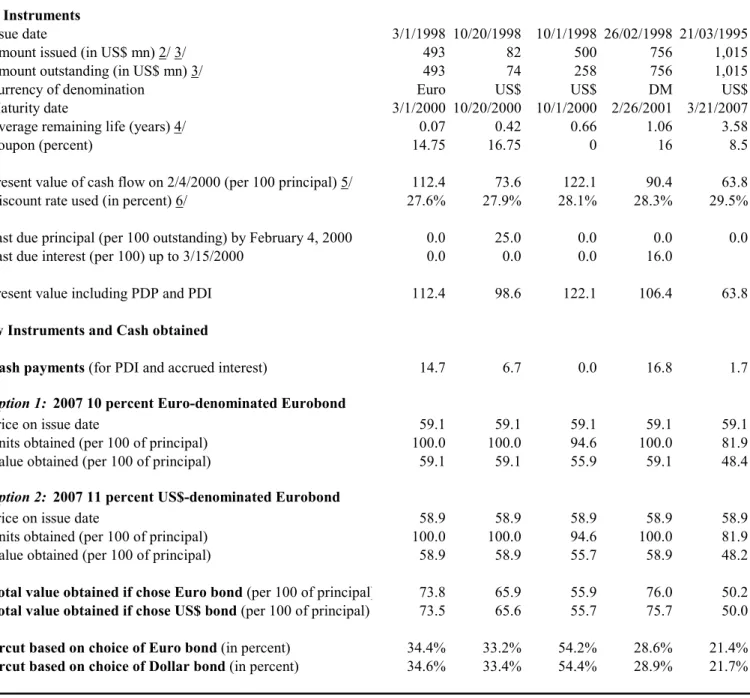
On February 4, 2000, with ING Barings as lead manager, Ukraine launched a comprehensive exchange offer involving all outstanding commercial bonds. This included a Euro 500 million, 14.75 percent Eurobond due in March 2000, the restructured $74 million 16.75 percent Chase Manhattan bond maturing in October 2000, the remainder of a restructured Merrill Lynch Eurobond (US$258.4 million) falling due in October of 2000, and the DM 1.5 billion, 16 percent Eurobond due in February 2001. In addition, there were about $1 billion of 8.5 percent bonds owed to the Russian energy exporter Gazprom falling due between March of 2000 and March of 2007.
Creditors could choose between two 7-year coupon amortization bonds denominated either in Euros or U.S. dollars, to be issued under English law. For the Euro denominated bond, the coupon was set at 10 percent, while for the U.S. dollar denominated bond it was set at 11 percent. The was no face value reduction except for the zero coupon Merrill Lynch Eurobond, where it was about 5 percent and for the “Gazprom bonds”, where it ranged between 0 and 33 percent depending on the maturity date of the bonds. Coupon payments for the new bonds were set on a quarterly basis, with no grace period for interest payments. Amortization was to occur twice a year, with 3 percent at each amortization date in 2001, 5 percent in 2002, and 9.33 percent at each date between 2003 and 2007. Past due interest and accrued interest (i.e. interest accrued since the last scheduled coupon payment which was not yet payable) was paid in full and in cash. The exchange offer established a minimum participation threshold of 85 percent among the holders of bonds maturing in 2000-2001. In the event, there was almost full participation.
In Table 5 all claims (present values of old instruments, past due interest and principal, cash payments, and the number of units of new instruments received) are computed for 100 units of principal outstanding at the time of the exchange.20 In addition to one case of past due interest (on the DM Eurobond, whose annual 16 percent coupon payment was missed in February 2000), there is a case of past due principal from a missed amortization payment due in January 2000; according to the IMF (2001), these payments were missed for “intercreditor equity” reasons, i.e. to avoid paying some investors in full during or immediately before a debt restructuring offer. Note that while past due interest and principal need to added to the forward looking present value of the old instrument in order to establish the total claim, accrued interest is automatically reflected in the present value, since it is embodied in the first coupon payment coming due.
One difficulty compared to the case of Russia is that only the two newly issued Eurobonds were trading in the market after the exchange; thus, it is not possible to interpolate yields based on a full Eurobond yield curve for the purpose of discounting, as was the case for Russia. Instead, the yields used for discounting are those of the actual new instruments used to exchange each of the old bonds, with a small maturity adjustment based on the U.S. yield curve.
20 Thus, for the amortizing Chase Manhattan loan shown in the second column, present values, PDP, etc. are
expressed as percentages of the principal that had not been repaid by February of 2000 (89 percent of the original principal).
- 19 - OVDP Domestic Holders OVDP International
Holders Chase Manhattan ING Loan Old Instruments
Issue date 08/19/98 08/18/98 10/20/97 08/09/98
Amount issued (US$ mn) 9 35 109 163
Amount outstanding (US$ mn) 1 35 109 163
Maturity date 05/12/99 08/18/99 10/20/98 07/09/99
Coupon (percent) 0.0 0.0 10.0 17.5
Discount rate used (yield, in percent) 64.9% 60.5%
Present value on 8/98 (per 100 principal) 68.73 62.30
Present value on 10/98 (per 100 principal) 100.00
Present value on 8/99 (per 100 principal) 100.00
New Instruments and Cash obtained
Recognized value of old instrument (per $100 of Principal) 68.73 62.30 100.00 100.00
Discount rate used (yield, in percent): 54.8% 74.1% 76.3% 81.6%
Cash Payment
Per $100 of Principal 0.00 0.00 25.00 20.00
Lower Bound - Shortest Maturity 8/26/2001 (68.7% of total recognized value)
Per $100 of Principal 63.40
Upper Bound - Longest Maturity 8/26/2004 (68.7% of total recognized value)
Per $100 of Principal 63.67
Eurobond Merrill Lynch 8/26/2000 (62.3% of total recognized value)
Per $100 of Principal 29.59
Chase Manhattan 10/20/2000 (75% of total recognized value)
Per $100 of Principal 44.34
ING Loan 2/26/2001 (80% of total recognized value)
Per $100 of Principal 44.51
Lower Bound - Total Value received 63.40
Upper Bound - Total Value received 63.67
Eurobond Merrill Lynch - Total Value received 29.59
Chase Manhattan - Total Value received 69.34
ING Loan - Total Value received 64.51
Haircuts based on shotest 3 years bond (lower bound) 7.8%
Haircut based on longest 6 years bond (upper bound) 7.4%
Haircut - Eurobond Merrill Lynch 52.5%
Haircut - Chase Manhattan 30.7%
Haircut - ING Loan 35.5%
Table 4. Ukraine Domestic Exchanges August 1998 - August 1999
2000 US$ Chase Merrill - 2001 DM Gazprom Eurobond Manhattan Lynch Eurobond bonds 1/ Old Instruments
Issue date 3/1/1998 10/20/1998 10/1/1998 26/02/1998 21/03/1995
Amount issued (in US$ mn) 2/ 3/ 493 82 500 756 1,015
Amount outstanding (in US$ mn) 3/ 493 74 258 756 1,015
Currency of denomination Euro US$ US$ DM US$
Maturity date 3/1/2000 10/20/2000 10/1/2000 2/26/2001 3/21/2007
Average remaining life (years) 4/ 0.07 0.42 0.66 1.06 3.58
Coupon (percent) 14.75 16.75 0 16 8.5
Present value of cash flow on 2/4/2000 (per 100 principal) 5/ 112.4 73.6 122.1 90.4 63.8
Discount rate used (in percent) 6/ 27.6% 27.9% 28.1% 28.3% 29.5%
Past due principal (per 100 outstanding) by February 4, 2000 0.0 25.0 0.0 0.0 0.0
Past due interest (per 100) up to 3/15/2000 0.0 0.0 0.0 16.0
Present value including PDP and PDI 112.4 98.6 122.1 106.4 63.8
New Instruments and Cash obtained
Cash payments (for PDI and accrued interest) 14.7 6.7 0.0 16.8 1.7
Option 1: 2007 10 percent Euro-denominated Eurobond
Price on issue date 59.1 59.1 59.1 59.1 59.1
Units obtained (per 100 of principal) 100.0 100.0 94.6 100.0 81.9
Value obtained (per 100 of principal) 59.1 59.1 55.9 59.1 48.4
Option 2: 2007 11 percent US$-denominated Eurobond
Price on issue date 58.9 58.9 58.9 58.9 58.9
Units obtained (per 100 of principal) 100.0 100.0 94.6 100.0 81.9
Value obtained (per 100 of principal) 58.9 58.9 55.7 58.9 48.2
Total value obtained if chose Euro bond (per 100 of principal) 73.8 65.9 55.9 76.0 50.2
Total value obtained if chose US$ bond (per 100 of principal) 73.5 65.6 55.7 75.7 50.0
Haircut based on choice of Euro bond (in percent) 34.4% 33.2% 54.2% 28.6% 21.4%
Haircut based on choice of Dollar bond (in percent) 34.6% 33.4% 54.4% 28.9% 21.7%
1/ Simple average, i.e. synthetic instrument consiting of all 29 outstanding Gazprom bonds in equal parts. 3/ Evaluated using February 4, 2000 market exchange rates
4/ Weighted average of time of amortization, using percent amortization in each time period as weights.
6/ Yield to maturity of new bond of corresponding currency, with minor maturity adjustment based on US yield curve. Table 5. Ukraine External Debt Exchange
(February 4-April 7, 2000)
2/ For Chase Manhattan loan, the difference between amounts issued and outstanding is due to amortization during 1999. For Merrill Lynch bond, it is due to the retiring of principal after July 1999 exchange offer.
- 21 -
The main result is that while in this case there were no significant nominal haircuts except on some of the “Gazprom bonds”, the present value losses were significant, ranging from about 22 to 54 percent. Not surprisingly, the haircut did not depend much on which of the two new bonds was chosen by investors. However, it varied quite significantly across the old bonds. Two main facts stand out: first, the haircut suffered by the Merrill Lynch bond (54 percent) stands out. In an accounting sense, this is due to the fact that the PV of the cash flow of this bond was higher than the rest, with a large nominal return of 44 percent expected in October, while the terms of restructuring were slightly worse (perhaps because it was felt that since a zero coupon bond was being exchanged for an 11 percent coupon bond, a small face value reduction was appropriate). Second, except for the Merrill Lynch bond, bonds with shorter life suffered larger haircuts than bonds with longer life. This can be observed both for the bonds shown and within the class of Gazprom bonds. Thus, the larger nominal haircuts applied to longer dated Gazprom bonds did not completely offset the smaller present values of the longer bonds at the discount rates applied in our calculations. We return to this point in the last section of the paper.
C. Pakistan21
Pakistan’s 1999 Eurobond restructuring originated from a history of high public debt (about 90 percent of GDP since the early 1990s) and a major balance of payments crisis in May of 1998 triggered by international sanctions imposed after a series of nuclear tests. After the lifting of most sanctions in late 1998, Pakistan negotiated a Paris Club restructuring in January of 1999 which required the country to seek comparable debt relief from private creditors, and in particular, to restructure its international bonds. By July, the government had signed a rescheduling with commercial banks covering about $900 million in commercial loans, but it held off on restructuring its Eurobonds, as no principal repayments were coming due until the end of the year. Finally, on November 15, Pakistan launched a bond exchange, ahead of a Paris club deadline that required it to show “progress” in negotiations with bondholders by the end of 1999. No interest or principal payments were missed prior to the exchange.
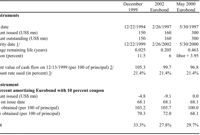
The exchange involved swapping three bonds: a $150 million, 11.5 percent Eurobond due in December 1999; a $160 million, 6 percent exchangeable note due in February 2002 with a put option in February 2000; and a $300 million Libor-plus-3.95 percent floating rate note due in May of 2000. All three would be exchanged for a new amortizing bond with an overall maturity of six years and a three-year grace period, paying a 10 percent coupon. There was no nominal haircut; in fact, holders of the two bonds with the shorter average life received slightly more in nominal terms than under the original instruments (Table 6).
21
This chapter relies on Helbling (2001), Burki (2000), IMF Country Reports No. 97/120, 01/11, 01/24, 01/222 and 03/338, the IMF Staff Report for the 1998 Article IV consultation (unpublished but publicly available under the IMF’s policy of releasing most Executive Board documents that are more than five years old) financial sector newsletters and news reports.
Table 6 is similar in structure but simpler than most of the previous tables, as there was only one exchange option and no need to reimburse past due interest or principal. Haircuts were of about the same order as the average haircut in the case of Ukraine, i.e. about 30 percent. Unlike Ukraine, however, there was not much variation in the magnitude of haircuts across the old instruments. In this respect, the Pakistan exchange resembles the Russian PRINs and IANs exchange. Also as in the case of Russia, the remaining life of the original instruments was almost the same across instruments (in this case, very short).
Old Instruments
Issue date 12/22/1994 2/26/1997 5/30/1997
Amount issued (US$ mn) 150 160 300
Amount outstanding (US$ mn) 150 160 300
Maturity date 1/ 12/22/1999 2/26/2002 5/30/2000
Average remaining life (years) 0.025 0.205 0.463
Coupon (percent) 11.5 6 libor + 3.95
Present value of cash flow on 12/13/1999 (per 100 of principal) 2/ 105.3 99.7 96.8
Discount rate used (in percent) 3/ 21.4% 21.4% 21.4%
New Instrument
2005 percent amortizing Eurobondwith 10 percent coupon
Amount issued (US$ mn) -4.8 -9.1 0.0
Price on issue date 68.1 68.1 68.1
Units obtained (per 100 of principal) 103.2 105.7 100.0
Value obtained (per 100 of principal) 70.3 72.0 68.1
Haircut 33.3% 27.8% 29.7%
1/ 2002 Bond had put option in February 2000.
3/ Yield to maturity on new 2005 Eurobond, with a minor maturity correction based on the US yield curve. 2/ Includes accrued interest. For puttable 2002 bond, we assume that the option to put would have been used for entire outstanding amount in February of 2000
Table 6. Pakistan Eurobond Exchange (November 15-December 13, 1999) December 1999 2002 Eurobond May 2000 Eurobond
- 23 -
D. Ecuador22
Ecuador’s debt crisis occurred less than five years after a Brady deal with commercial banks had reduced the country’s external debt to sustainable, though still high, debt levels. It originated in a banking crisis that erupted in April of 1998 and became progressively worse due to a lack of crisis resolution instruments and political obstacles. Central Bank liquidity support to failing banks put pressure led to a currency crisis in early 1999, and by mid-1999, net international reserves had fallen to levels that made it very difficult to meet upcoming debt service payments—about $550 million on Brady and Eurobonds during the remainder of 1999 and 2000, and maturing domestic debt in the order of US$500 million—without agreement on an IMF program. But the IMF in turn required some degree of “private sector bail-in” to help close the financing gap and return to sustainable debt levels.
Against this background, on August 25, 1999, Ecuador announced that it would suspend coupon payments on Discount and PDI Brady bonds. After a failed attempt to persuade the Brady bondholders to accept a debt exchange limited to Brady bonds, Ecuador also defaulted on its remaining Brady bonds and, by the end of October, on its Eurobonds. It was the first default on international sovereign bonds since the 1930s (previous postwar defaults— including during the 1980s debt crisis, and the Russian and Ukrainian defaults of 1998–– had affected only commercial bank loans and domestic debt). In addition, about US$ 500 million of short-term domestic dollar-denominated debt was restructured to longer maturities at a reduced rate of interest.23
With IMF support, on July 27, 2000, Ecuador launched an offer to exchange its defaulted Brady Bonds and Eurobonds for new uncollateralized bonds maturing in 2030 with a step-up coupon starting at 4 percent and rising to 10 percent, in 1 percent steps, by 2006 (Table 7). For each type of defaulted bond, an exchange ratio was set in line with “stripped” secondary market prices; thus, the idea was to treat each bond equally based on their pre-default prices. The shortest instruments, namely Eurobonds and Brady Interest Equalization bonds were exchanged at par, while the longer dated Brady bonds were exchanged at 1:0.78 (PDI bonds), 1:0.58 (Discount bonds) and 1:0.40 (Pars). Holders of Par and Discount bonds also received a cash payment equal to the present value of their U.S. collateral. Past due interest and principal were repaid in cash, while accrued interest (interest owed since the last scheduled coupon payment) was exchanged, at par, for a new Republic bond with a fixed coupon of 12 percent, maturing in 2012. Bondholders could also elect to exchange their principal for this shorter bond rather than the 2030 bonds at the price of a further 35 percent discount relative to the face value of the 2030 bonds. The aggregate amount of 2012 bonds was limited to 1.25 billion, and holders of Eurobonds and shorter dated Brady bonds were given priority in the
22 This chapter is based on Jacome (2004), Fischer (2001), Beckerman (2002), Bucheit (2000), IMF Staff
Country Reports, and news reports.
23 IMF (2002) suggests that the PV loss in the domestic exchange was 9% but we have not been able to confirm
allocation of the 2012 bonds. By the time the exchange was finalized on August 23, over 97 percent of the eligible bonds had agreed to tender.
Two technical issues in Table 7 are worth mentioning. First, although our general principle is to compute the present value of the old instruments using the yield on the new instruments as the discount rate, the 2025 principal repayments scheduled for the Par and Discount bonds are discounted using the US long treasury bill rate, since these repayments were collateralized and not subject to country risk. Ceteris paribus, collateralization thus increases the present value of the old instruments and the value received in the exchange in equal measure (since the latter involved the release of the collateral), which means that it has no effect on the haircut, which is the percentage difference between the two.
- 25 -
Pars Discounts PDIs IEs 2002 Euro 2004 Euro
Old Instruments
Issue date 02/28/1995 02/28/1995 02/28/1995 12/21/1994 04/25/1997 04/25/1997
Amount issued (US$ mn) 1,655 1,435 2,308 191 350 150
Amount outstanding (US$ mn) 1/ 1,655 1,435 2,775 143 350 150
Maturity date 02/28/2025 02/28/2025 02/27/2015 12/21/2004 04/25/2002 04/25/2004
Average remaining life (years) 2/ 24.5 24.5 10.59 2.56 1.67 3.67
Coupon (percent) 3-5 step up libor+13/16 libor+13/16 libor+13/16 11.25 libor +4.75
Present value of cash flow on August 23 (PV1) 3/ 49.0 66.3 46.4 76.6 90.1 79.8
Discount rate used (in percent) 4/ 21.1 21.1 21.8 22.6 22.6 22.6
Present value of cash flow on August 23 (PV2) 3/ 48.5 64.8 45.0 75.5 89.2 78.5
Discount rate used (in percent) 5/ 21.6% 22.0% 22.4% 23.4% 23.5% 23.3%
Past due principal (PDP, per 100 of principal) 0.00 0.00 0.00 10.00 0.00 0.00
Past due interest (PDI, per 100 principal) 6/ 4.10 4.68 1.96 7.29 12.05 11.25
PV1 + PDI + PDP 53.1 70.9 48.3 93.9 102.2 91.0
PV2 + PDI + PDP 52.6 69.4 46.9 92.8 101.2 89.7
New Instruments and Cash obtained Cash payments
Release of principal collateral (per 100 of principal) 23.5 23.5 0.0 0.0 0.0 0.0
Payment for PDI and PDP (per 100 of principal) 4.1 4.7 2.0 17.3 12.0 11.3
2030 Eurobond with 4/5/6/7/8/9/10 percent step-up coupon
Amounts issued (US$ mn) 7/ 662.0 832.3 1169.4 0.0 0.0 0.0
Price on issue date 36.2 36.2 36.2 36.2 36.2 36.2
Units obtained for principal (per 100 of principal) 40.0 58.0 78.0 100.0 100.0 100.0
Value obtained for principal (per 100 of principal) 14.5 21.0 28.2 36.2 36.2 36.2
2012 Eurobondwith 12 percent coupon
Amounts issued (US$ mn) 7/ 15.6 50.7 745.0 95.1 240.4 103.2
Price on issue date 60.2 60.2 60.2 60.2 60.2 60.2
Units obtained for accrued interest (per 100 princ.) 0.9 3.5 3.5 1.4 3.7 3.8
Value obtained for accrued interest (per 100 princ.) 0.6 2.1 2.1 0.8 2.2 2.3
if elected instead of 2030 bonds:
Units obtained for principal (per 100 of principal) 26.0 37.7 50.7 65.0 65.0 65.0
Value obtained for principal (per 100 of principal) 15.7 22.7 30.5 39.1 39.1 39.1
Total value obtained 42.6 51.3 33.4 57.3 53.4 52.7
Haircut based on PV1 (in percent) 19.7% 27.7% 30.9% 39.0% 47.7% 42.2%
Haircut based on PV2 (in percent) 19.0% 26.1% 28.9% 38.3% 47.2% 41.3%
2/ Weighted average of time of amortization, using percent of remaining amortization in each time period as weights. 3/ Including accrued interest
6/ Including interest on principal and interest arrears.
5/ Yield corresponding to average life, using linear interpolation of outstanding Eurobond yields. For Pars and Discounts, 2025 principal was discounted using US long rate.
7/ Based on the assumption that all bondholders opted for the 2012 bond and were rationed as announced in the exchange offer (i.e. shorter instruments had priority; the 2012 would be prorated within the marginal class, i.e. PDI bonds).
Table 7. Ecuador Exchange (July 27-August 23, 2000)
1/ For PDIs, difference between amount issued and outstanding is due to capitalization of interest payments prior to the exchange; for IEs, difference is due to amortization payments made between June 1995 and June 1999.
4/ Yield of new bond actually used to exchange principal of respective old bond (2030 for Pars and Discounts, 2012 for IEs and Eurobonds, and a mix for the PDI bond). For Pars and Discounts, 2025 principal was discounted using US long rate.
Second, unlike in the Ukrainian exchange, past due principal—which existed for IE bonds, which were amortizing bonds—was repaid in cash. As a result, the present values of old instruments, number of units of new instruments, etc. shown for the IE bonds refer to 100 units of principal outstanding after repayment of PDP, which was 65 percent of the original principal. Similarly, for PDI bonds, which were capitalizing bonds (part of the coupon payments were rolled into a rising principal amount) the values refer to the principal outstanding at the time of the exchange, which as about 118 percent of the original principal. The main results are as follows. As expected, the 2012 option delivered a slightly higher value (compare lines “value obtained for principal” for the 2030 and 2012 bonds), and thus was rationed. As in the case of Ukraine, there were substantial differences in the haircuts across instruments, ranging between 19 and 48 percent. Again, the bonds with the longest remaining average life tend to suffer the smallest NPV haircuts (in the 20-30 percent range), while the largest haircuts are associated with the shortest instruments, notwithstanding the fact that the longer instruments were subjected to larger reductions in face value. Ex post, it turns out that these reductions were insufficient to equalize the NPV haircuts; consequently, there is a negative correlation between NPV haircuts and nominal haircuts.
Aside from being the first debt exchange to involve Brady bonds, Ecuador’s exchange was innovative in several respects. The new bonds contained two novel features meant to minimize the chances of a new debt restructuring in the foreseeable future and protect the interests of bondholders. A “mandatory debt management” provision committed Ecuador to retiring a minimum proportion of the face value of each of the new bonds every year. A “principal reinstatement” provision meant that a payment default occurring in the first 10 years would automatically result in the issuance of additional 2030 bonds to the holders. The effect of this was to offer a (limited) protection of bondholders against the dilution of their claims by new debt holders in the event of default. Finally, for the first time in sovereign debt, the Ecuador exchange used “exit amendments” to put pressure on potential holdouts. As part of the exchange, Ecuador solicited the consent of existing bondholders to change various non-payment terms of the old instruments, which (unlike the payment terms) could be changed with simple majority, with the effect of reducing the liquidity of non-tendered bonds and stripping them from various creditor protections.
E. Argentina
In November 2001, after several attempts at balancing the budget and avoiding a restructuring of debt obligations, a substantial reduction in tax collection together with the lack of additional access either to market or multilateral funds forced the government to seek debt relief through a “voluntary” exchange in two stages. The first stage (Phase 1) would be targeted at domestic residents and the second (Phase 2) to nonresidents. The idea was to segment local and foreign bondholders to protect the local financial institutions and domestic pension funds by guaranteeing the resources to honor the obligations with them. In the end, Phase 1 did happen, but shortly after the government was ousted in a civilian coup that decided on a broader default; thus Phase 2 never materialized.