Dissertations
2017
Distributed nonconvex optimization: Algorithms
and convergence analysis
Davood Hajinezhad
Iowa State UniversityFollow this and additional works at:
https://lib.dr.iastate.edu/etd
Part of the
Operational Research Commons
This Dissertation is brought to you for free and open access by the Iowa State University Capstones, Theses and Dissertations at Iowa State University Digital Repository. It has been accepted for inclusion in Graduate Theses and Dissertations by an authorized administrator of Iowa State University Digital Repository. For more information, please [email protected].
Recommended Citation
Hajinezhad, Davood, "Distributed nonconvex optimization: Algorithms and convergence analysis" (2017).Graduate Theses and Dissertations. 16140.
by
Davood Hajinezhad
A dissertation submitted to the graduate faculty in partial fulfillment of the requirements for the degree of
DOCTOR OF PHILOSOPHY
Major: Industrial Engineering
Program of Study Committee: Mingyi Hong, Co-major Professor
Gary Mirka, Co-major Professor Sarah Ryan
Sigurdur Olafsson Zhengdao Wang
Peng Wei
The student author, whose presentation of the scholarship herein was approved by the program of study committee, is solely responsible for the content of this dissertation. The Graduate College will ensure this dissertation is globally accessible and will not permit alterations after a degree is
conferred.
Iowa State University Ames, Iowa
2017
DEDICATION
This dissertation is for my beloved wife, Elham. Thanks for being always with me, for your love, and endless support in this long trip.
TABLE OF CONTENTS
Page
LIST OF TABLES . . . vii
LIST OF FIGURES . . . viii
ACKNOWLEDGEMENTS . . . x
ABSTRACT . . . xi
CHAPTER 1. INTRODUCTION . . . 1
CHAPTER 2. PROXIMAL PIMAL-DUAL ALGORITHM FOR DISTRIBUTED NONCON-VEX OPTIMIZATION . . . 10
2.1 Introduction . . . 10
2.2 The Prox-PDA Algorithm . . . 13
2.3 The Convergence Analysis . . . 14
2.4 Variants of Prox-PDA . . . 19
2.5 Connections and Discussions . . . 21
2.6 Distributed Matrix Factorization . . . 22
2.7 Numerical Results . . . 27
2.7.1 Distributed Binary Classification . . . 27
2.7.2 Distributed Matrix Factorization . . . 28
2.8 Appendix. Lemma proofs . . . 29
2.8.1 Proof of Lemma23 . . . 29
2.8.2 Proof of Lemma2 . . . 29
2.8.3 Proof of Lemma3 . . . 30
2.8.5 Proof of Lemma25 . . . 32
2.8.6 Proof of Theorm1 . . . 33
2.8.7 The Analysis Outline for Prox-GPDA . . . 35
2.8.8 Proof of Convergence for Prox-PDA-IP . . . 36
2.8.9 Proof of Convergence for Algorithm2 . . . 44
CHAPTER 3. A NONCONVEX PRIMAL-DUAL SPLITTING METHOD FOR DISTRIBUTED AND STOCHASTIC OPTIMIZATION . . . 50
3.1 Introduction . . . 50
3.2 The NESTT-G Algorithm . . . 54
3.3 The NESTT-E Algorithm . . . 58
3.4 Connections and Comparisons with Existing Works . . . 60
3.5 Numerical Results . . . 62 3.6 Appendix. Proofs . . . 64 3.6.1 Proof of Lemma6 . . . 66 3.6.2 Proof of Theorem4 . . . 70 3.6.3 Proof of Theorem5 . . . 73 3.6.4 Proof of Theorem6 . . . 79 3.6.5 Proof of Proposition 1. . . 86
CHAPTER 4. PERTURBED PROXIMAL PRIMAL DUAL ALGORITHM FOR NON-CONVEX NONSMOOTH OPTIMIZATION . . . 88
4.1 Introduction . . . 88
4.1.1 Motivating Applications . . . 89
4.1.2 Literature Review and Contribution. . . 91
4.2 Perturbed Proximal Primal Dual Algorithm . . . 95
4.2.1 Convergence Analysis . . . 96
4.2.2 The Choice of Perturbation Parameter . . . 104
4.3 An Algorithm with Increasing Accuracy . . . 111
4.4 Numerical Results . . . 125
4.4.1 Distributed Nonconvex Quadratic Problem . . . 125
4.4.2 Nonconvex subspace estimation . . . 127
4.4.3 Partial Consensus . . . 130
4.5 Conclusion . . . 131
4.6 Appendix. Constraint qualification . . . 132
CHAPTER 5. ZEROTH ORDER NONCONVEX MULTI-AGENT OPTIMIZATION . . . . 138
5.1 INTRODUCTION . . . 138
5.2 Zeroth-Order Algorithm over MNet . . . 144
5.2.1 System Model . . . 144
5.2.2 The Proposed Algorithm . . . 146
5.2.3 The Convergence Analysis of ZONE-M . . . 149
5.3 Zeroth-Order Algorithm over SNet . . . 153
5.3.1 System Model . . . 154
5.3.2 Proposed Algorithm . . . 154
5.3.3 Convergence Analysis of ZONE-S . . . 155
5.4 Numerical Results . . . 158
5.4.1 ZONE-M Algorithm . . . 158
5.4.2 ZONE-S Algorithm . . . 160
5.5 Conclusion . . . 161
5.6 Appendix. Proofs for ZONE-M . . . 162
5.6.1 Proof of Lemma 23 . . . 162
5.6.2 Proof of Lemma 24 . . . 163
5.6.3 Proof of Lemma 25 . . . 166
5.6.4 Proof of Theorem 9 . . . 168
5.7.1 Proof of Lemma 26 . . . 175 5.7.2 Proof of Theorem 10 . . . 177
LIST OF TABLES
Page
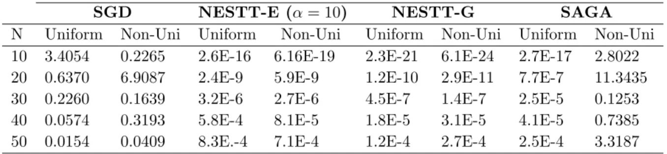
Table 3.1 Comparison of # of gradient evaluations for NESTT-G and GD in the worst case . . . 87 Table 3.2 Optimality gapk∇˜1/βf(zr)k2for different algorithms, with 100 passes of the
datasets. . . 87 Table 4.1 Comparison of proposed algorithms with DSG algorithm. Alg1 and Alg2
denote PProx-PDA and PProx-PDA-IA algorithms respectively. . . 127 Table 4.2 Comparison of PPox-PDA-IA with ADMM in terms of Global Error kΠˆ −
Π∗k for nonconvex subspace estimation problem with MCP Regularization. 130 Table 4.3 Recovery results for PPox-PDA-IA and ADMM in terms of TPR and FPR. 130
LIST OF FIGURES
Page
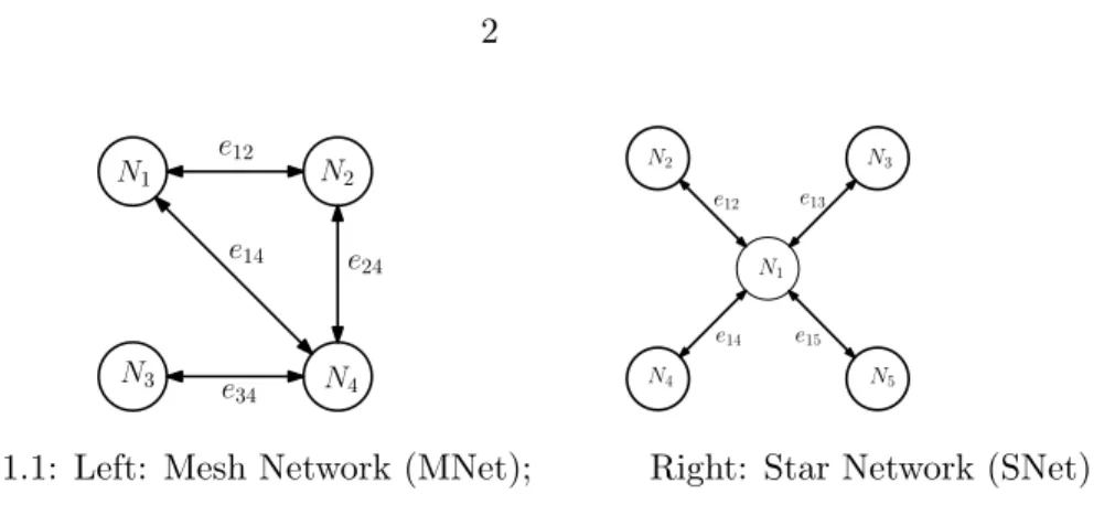
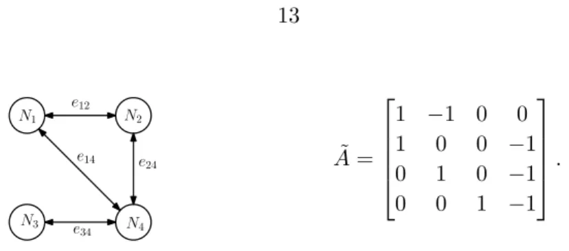
Figure 1.1 Left: Mesh Network (MNet); Right: Star Network (SNet) . . . 2 Figure 1.2 Splitting data matrix across the rows . . . 3 Figure 2.2 (Left) An undirected Connected Network, (Right) Incidence Matrix. . . . 13 Figure 2.3 Results for the matrix factorization problem. . . 27 Figure 2.4 Results for the matrix factorization problem. . . 27
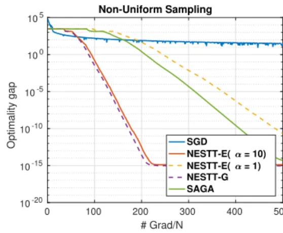
Figure 3.2 Comparison of NESTT-G/E, SAGA, SGD on problem (3.22) . . . 63
Figure 4.1 Comparison of proposed algorithms with DSG [102] and NEXT [92] in terms of stationary gap for problem4.114 with parametersN = 20, R= 0.7, d = 10, α= 0.01. . . 127 Figure 4.2 Comparison of proposed algorithms with DSG [102] and NEXT [92] in terms
of constraint violation for problem 4.114 with parameters N = 20, R = 0.7, d= 10, α= 0.01. . . 127 Figure 4.3 Comparison of proposed algorithms with ADMM in terms of stationary gap
for nonconvex subspace estimation problem with MCP Regularization. The solid lines and dotted lines represent the single performance and the average performance, respectively. . . 128 Figure 4.4 Comparison of proposed algorithms with ADMM in terms of constraint
vio-lationkAxk2 for nonconvex subspace estimation problem with MCP Regu-larization. The solid lines and dotted lines represent the single performance and the average performance, respectively. . . 128
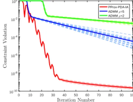
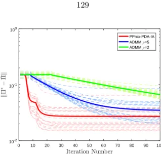
Figure 4.5 Comparison of proposed algorithms with ADMM in terms of Global Error for non-convex subspace estimation problem with MCP Regularization. The problem parameters aren= 80,p= 128, ν = 3, b= 3. The solid lines and dotted lines represent the single performance and the average performance,
respectively. . . 129
Figure 4.6 The stationary gap achieved by the proposed methods for the partial con-sensus problem. The solid lines and dotted lines represent the single perfor-mance and the average perforperfor-mance, respectively. . . 131
Figure 4.7 Constraint ViolationkAxkachieved by the proposed methods for the partial consensus problem with different permissible toleranceζ. . . 131
Figure 5.1 Left: Mesh Network (MNet); Right: Star Network (SNet) . . . 141
Figure 5.3 The optimality gap versus iteration counter . . . 160
Figure 5.4 The constraint violation versus iteration counter . . . 160
Figure 5.5 Comparison of different algorithms for the nonconvex consensus problem given in (5.58). . . 160
ACKNOWLEDGEMENTS
With immense appreciation, I would like to express my gratitude to the people who helped me to bring this study into success.
First, my major professor, Dr. Mingyi Hong for valuable guidance, boundless knowledge, con-sistent advices, patience, and continuous support in all aspects of my PhD life. You certainly provided me with the necessary tools that I needed to successfully complete my graduate program and this dissertation.
Additionally I would like to acknowledge my committee members Dr. Mirka, Dr. Ryan, Dr. Olafsson form Industrial and Manufacturing System Engineering department, Dr. Wang from Electrical and Computer Engineering department, and Dr. Wei from Aerospace Engineering de-partment. Your feedbacks definitely improved the quality of my research.
Finally, topmost gratitude to my parents. You are always there for me. Doubtlessly, I was not here without your love and spiritual supports throughout my life.
ABSTRACT
This thesis addresses the problem of distributed optimization and learning over multi-agent networks. Our main focus is to design efficient algorithms for a class of nonconvex problems, defined over networks in which each agent/node only has partial knowledge about the entire problem. Multi-agent nonconvex optimization has gained much attention recently due to its wide applications in big data analysis, sensor networks, signal processing, multi-agent network, resource allocation, communication networks, just to name a few. In this work, we develop a general class of primal-dual algorithms for distributed optimization problems in challenging setups, such as nonconvexity in loss functions, nonsmooth regularizations, and coupling constraints. Further, we consider different setup where each agent can only access the zeroth-order information (i.e., the functional values) of its local functions. Rigorous convergence and rate of convergence analysis is provided for the proposed algorithms. Our work represents one of the first attempts to address nonconvex optimization and learning over networks.
CHAPTER 1. INTRODUCTION
This research mainly focuses on designing algorithms for distributed nonconvex optimization problems under different network topologies. Distributed nonconvex optimization problem has found a wide range of applications in several areas, including data-intensive optimization [65, 146], signal and information processing [47, 117], multi-agent network resource allocation [134], commu-nication networks [82], just to name a few. In particular, it is a key enabler of many emerging “big data” analytic tasks. In these data-intensive applications, the sheer volume and spatial/temporal disparity of big data render centralized processing and storage a formidable task. This happens, for instance, whenever the volume of data overwhelms the storage capacity of a single comput-ing device. Moreover, collectcomput-ing sensor-network data, which are observed across a large number of spatially scattered centers/servers/agents, and routing all this local information to centralized processors, under energy, privacy constraints and/or link/hardware failures, is often infeasible or inefficient. Further, with the advent of high performance and parallel computing interfaces it is reasonable to model the problem such that we are able to utilize these interfaces to accelerate the computations.
Typically, distributed optimization problem can be expressed as minimizing the sum of addi-tively separable cost functions plus a regularization function, given below
min x∈X g(x) := N X i=1 fi(x) +h(x), (1.1)
whereN denotes the number of agents in the network; fi:RM →Rrepresents some cost function
related to the agent i,X ⊂RM is a convex set, and h(x) imposes some regularity such as sparsity
to the solution, or denotes the indicator function of a convex set. It is usually assumed that each agentihas complete information onfi, and it can only communicate with its neighbors. Therefore
the key objectives of the individual agents are: 1) to achieve consensus with its neighbors about the optimization variable; 2) to optimize the global objective functiong(x).
e12 e24 e14 e34 N1 N2 N4 N3 e15 e13 e12 e14 N4 N5 N3 N2 N1
Figure 1.1: Left: Mesh Network (MNet); Right: Star Network (SNet)
We consider two popular network topologies, namely, the mesh network (MNet) (cf. Fig. 1.1 Left) and the star network (SNet) (cf. Fig. 1.1 Right). In the MNet, each node is connected via undirected links to a subset of nodes. Such a network is very popular in a number of applications. For example, in distributed signal processing [47, 117], each node can represent a sensor which has limited communication capability hence can only talk to its neighbors. On the other hand, SNet contains a central controller (i.e., the parent) which is connected to all other nodes (i.e., the children), and there is no connection between the children. Such a network can be used to model parallel computing architecture in which each child represents a computing node, and the parent coordinates the computation of the children [145, 80, 55]. In our work, we consider these different network topologies not only because they are capable of modeling a wide range of applications, but more importantly, their unique characteristics lead to a number of open challenges in designing distributed algorithms.
Extensive research has been done on developing algorithms for distributed optimization (for both MNet and SNet), but these works are mostly restricted to the family of convex problems where
fi(x)’s are all convex functions (detailed literature review is relegated to the following chapters).
Once we go beyond the convexity, the literature is very scant. Therefore, this research is set out to fill such an important gap. Below we briefly describe three applications that motivate distributed nonconvex optimization.
• Distributed Sparse Principal Component Analysis. Principal component analysis (PCA) aims to reduce the dimension of multi-variate data set, and has a wide range of applications in science and engineering, see for example [50, 125, 121].
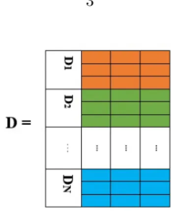
Figure 1.2: Splitting data matrix across the rows
Finding the first sparse principal component (PC) is equivalent to solving the following opti-mization problem
max kDxk22−λr(x), s.t.kxk22≤1 (1.2) where D ∈ RQ×M is a centered data matrix, and kDxk2
2 represents the explained variance of the first PC [72], r(x) is a sparsity-promoting regularizer, and λ > 0 is the penalization parameter. In practice, r(x) can take the form of the `0 norm of x, or its approximations such as the popular `1 norm, the log sum penalty (LSP) [22] and so on. In this research we consider the more challenging scenario where the data matrixD is not available in a central location, instead it is distributed over a network, and each agent has access to a mini-batch of the data points. In particular, letDi ∈RQi×M, i= 1,2,· · ·N denote submatrices that consist
non-overlapping rows (or data samples) ofD. That is,D= [D1;D2;· · ·;DN]; see Figure 1.2.
According to this data model, the SPCA problem (1.2) can be reformulated as follows
min N X i=1 −kDixk2 2+λr(x), s.t.kxk22≤1. (1.3)
This problem is nonconvex because−kDixk2
2 in the objective is a concave function. Further, it is easy to see that this problem has the same form as that of (1.1), withfi(x) =−kDixk22,
h(x) =λr(x), and X={x∈RM; s.t.kxk22≤1}.
• Distributed Nonlinear Regression Problem. This application is about a distributed regression problem. Consider the MNet, which consists ofN agents, and each agentihasQi
localobservation pairs (zij, bij);i= 1,2,· · · , N,j = 1,2,· · ·Qi. Suppose that each data point
is generated in the following manner:
bij =
1
1 + exp(−z>ijx) +ij,
where ij denotes the additive noise following a zero mean Gaussian distribution. Denote
hi(x, zij) = 1+exp(1−z> ijx)
, then we can form the following nonconvex nonlinear least square problem [91] min x N X i=1 Qi X j=1 [bij−hi(x, zij)]2+r(x), (1.4)
where againr(x) is a sparsity promoting regularizer. Clearly, problem (1.4) is a special case of (1.1), with fi(x) :=PjQ=1i [bij−hi(x, zij)]2.
• Distributed Target Localization Problem. Consider a network ofN agents collectively aim to locate M target points. Let’s xi ∈ Rd, i = 1,2,· · ·M denote the coordinate of the
each target location (d = 2 or 3). In target localization problem each agent i knows its own location wi, as well as a noisy measurement dij of the squared distance to each target
pointsj,j = 1,2,· · ·M. Therefore, this problem seeks to minimize the following nonconvex optimization problem [26] min x N X i=1 M X j=1 (dij − kxj−wik2)2, (1.5)
which is another special case of problem (1.1), withfi(x) =PMj=1(dij−kxj−wik2)2,h(x) = 0,
and X=RM.
The rest of this thesis contains three parts, as described below:
• Chapter 2. In this chapter we consider nonconvex optimization problem over the MNet (cf. Fig. 1.1). Typically this problem is modeled as the following
min x∈RM g(x) := N X i=1 fi(x), (1.6)
where eachfi,i∈ {1,· · ·, N}:= [N] is a nonconvex cost function. To solve this problem we
propose a proximal primal-dual algorithm (Prox-PDA). We show that Prox-PDA converges to the set of stationary solutions (satisfying the first-order optimality condition) in a globally sublinear manner. We also show that Prox-PDA can be extended in several directions to improve its practical performance. To the best of our knowledge, this is the first algorithm that is capable of achieving global sublinear convergence rate for distributed nonconvex opti-mization. Further, our work reveals an interesting connection between theprimal-dualbased algorithm Prox-PDA and the primal-onlyfast distributed algorithms such as EXTRA [122]. Finally, we generalize the theory for Prox-PDA based algorithms to a challenging distributed matrix factorization problem.
• Chapter 3. This chapter considers the SNet (given in Fig. 1.1Right). Utilizing SNet we are able to solve the following problem
min x∈X g(x) := 1 N N X i=1 fi(x) +f0(x) +p(x), (1.7) whereXis a closed and convex set; for eachi∈ {0,· · ·, N},fiis a smooth possibly nonconvex
function; p(x) is a lower semi-continuous convex but possibly nonsmooth function. Notice that in this problem we are able to deal with nonsmooth term p(x) as well as constraint set
X in contrast to the problem (1.6). We propose a class of NonconvEx primal-dual SpliTTing (NESTT) algorithms for this problem. The NESTT is one of the first stochastic algorithms for distributed nonconvex nonsmooth optimization, with provable and nontrivial convergence rates. The main contribution is the following. First, we show that NESTT converges sub-linearly to a point belongs to stationary solution set of (1.7). Second, we show that NESTT converges Q-linearly for certain nonconvex `1 penalized quadratic problems. To the best of our knowledge, this is the first time that linear convergence is established for stochastic and distributed optimization of such type of problems.
• Chapter 4. This chapter focuses on a general class of optimization problem given below min
wheref(x) :RN →Ris a continuous smooth function (possibly nonconvex); A∈RM×N is a
rank deficient matrix; b∈RM is a given vector; X is a convex compact set; h(x) :
RN →R
is a lower semi-continuous nonsmooth convex function.
Problem (1.8) subsumes a number of applications in the variety of domains, of which dis-tributed composite optimization problem over MNet including nonconvex loss functions and nonsmooth regularizations is a very important yet challenging problem. In what follows we show how distributed optimization problems in different setups can be cast in general formulation (1.8).
The exact consensus problem over networks. Consider a network which consists ofN
agents who collectively optimize the following problem min y∈R f(y) +h(y) := N X i=1 [fi(y) +hi(y)], (1.9)
wherefi(y) :R→Ris a smooth function, andhi(y) :R→Ris a convex, possibly nonsmooth
regularizer (here y is assumed to be scalar for ease of presentation). Note that both fi and
hi are local to agenti.
To integrate the structure of the network into problem (4.6), we consider MNet which is an undirected, connected graphG={V,E}, with|V|=Nvertices and|E|=Eedges. Each agent can only communicate with its immediate neighbors, and it is responsible for optimizing one component functionfi regularized by hi. Define the node-edge incidence matrix A∈RE×N
as following: if e ∈ E and it connects vertex i and j with i > j, then Aev = 1 if v = i,
Aev =−1 if v =j and Aev = 0 otherwise. Using this definition, thesigned graph Laplacian matrixL−∈RN×N is given by
L−:=ATA.
Introducing N new variables xi as the local copy of the global variable y, and define x :=
[x1;· · · ;xN]∈RN, problem (4.6) can be equivalently expressed as
min x∈RN f(x) +h(x) := N X i=1 fi(xi) +hi(xi) , s.t. Ax= 0. (1.10)
This problem is precisely original problem (1.8) with correspondenceX=RN,b= 0,f(x) :=
PN
i=1fi(xi), andh(x) :=
PN
i=1hi(xi).
The partial consensus problem. In the previous application, the agents are required to reachexact consensus, and such constraint is imposed throughAx= 0 in (4.7). In practice, however, consensus is rarely achieved exactly, for example due to potential disturbances in network communication; see detailed discussion in [75]. Further, in applications ranging from distributed estimation to rare event detection, the data obtained by the agents, such as harmful algal blooms, network activities, and local temperature, often exhibit distinctive spatial structure [28]. The distributed problem in these settings can be best formulated by using certain partial consensus model in which the local variables of an agent are only required to be close to those of its neighbors. To model suchpartial consensus constraint, we denote
ξe as the permissible tolerance for e= (i, j)∈ E, and replace the strict consensus constraint
xi−xj = 0 with kxi−xjk2 ≤ξe. Further, we define the link variable ze =xi−xj, and set
z := {ze}e∈E, Z := {z | kzek2 ≤ξe ∀ e∈ E}. Using these notations, the partial consensus
problem can be formulated as min x,z f(x) +h(x) := N X i=1 fi(xi) +hi(xi) (1.11) s.t. Ax−z= 0, z ∈Z,
which is again a special case of problem (1.8).
Notice that the application of optimization problem (1.8) are not limited to distributed op-timization problem. More problems such as sparse subspace estimation will be discussed in chapter Chapter4.
In Chapter4we develop an Uzawa type [74] algorithm named PProx-PDA for problem (1.8). One distinctive feature of the PProx-PDA is the use of a novel perturbation scheme for both the primal and dual steps, which is designed to ensure a number of asymptotic con-vergence and rate of concon-vergence properties (to first-order stationary solutions). Specifically, we show that when certain perturbation parameter remains constant across the iterations,
the algorithm converges globally sublinearly to the set of approximate first-order stationary solutions. Further, when the perturbation parameter diminishes to zero with appropriate rate, the algorithm converges to the set of exact first-order stationary solutions. To the best of our knowledge this is the first time that first-order methods with convergence and rate of convergence guarantees are developed for problems in the form of (1.8).
• Chapter 5. This chapter focuses on nonconvex distributed optimization problem under the challenging zeroth-order setup. A drawback for the algorithms in previous chapters is that they require at leastfirst-ordergradient information in order to guarantee global convergence. Unfortunately, in many real-world problems, obtaining such information can be very expen-sive, if not impossible. For example, in simulation-based optimization [126], the objective function of the problem under consideration can only be evaluated using repeated simulation. In certain scenarios of training deep neural network [76], the relationship between the decision variables and the objective function is too complicated to derive explicit form of the gradient. Further, in bandit optimization [2, 37], a player tries to minimize a sequence of loss functions generated by an adversary, and such loss function can only be observed at those points in which it is realized. In these scenarios, one has to utilize techniques from derivative-free optimization, or optimization using zeroth-order information [127, 27].
In this chapter we propose zeroth-order primal-dual based algorithms for distributed optimiza-tion problems over different network topologies. For MNet, we design an algorithm capable of dealing with nonconvexity and zeroth-order information simultaneously. It is shown that the proposed algorithm converges to the set of stationary solutions of problem (1.6) (with nonconvex but smooth fi’s), in a globally sublinear manner. Further, for SNet we propose
a stochastic primal-dual based method, which is able to further utilize the special structure of the network (i.e., the presence of the central controller) and deal with problem (1.7) with nonsmooth objective in zeroth-order setup. Theoretically, we show that this algorithm also converges to the set of stationary solutions in a globally sublinearly manner.
To the best of our knowledge, these algorithms are the first ones for distributed nonconvex optimization that are capable of utilizing zeroth-order information, while possessing global convergence rate guarantees.
CHAPTER 2. PROXIMAL PIMAL-DUAL ALGORITHM FOR DISTRIBUTED NONCONVEX OPTIMIZATION
Abstract
In this paper we consider nonconvex optimization and learning over a network of distributed nodes. We develop a Proximal Primal-Dual Algorithm (Prox-PDA), which enables the network nodes to distributedly and collectively compute the set of first-order stationary solutions in a global sublinear manner [with a rate ofO(1/r), wherer is the iteration counter]. To the best of our knowledge, this is the first algorithm that enables distributed nonconvex optimization with global rate guarantees. Our numerical experiments also demonstrate the effectiveness of the proposed algorithm.
2.1 Introduction We consider the following optimization problem
min z∈RM g(z) := N X i=1 fi(z), (2.1)
where eachfi,i∈ {1,· · · , N}:= [N] is a nonconvex cost function, and we assume that it is smooth
and has Lipschitz continuous gradient.
Such finite sum problem is of central importance in machine learning and signal/information processing [23, 47]. In particular, in the class of empirical risk minimization (ERM) problem, z
represents the feature vectors to be learned, and eachfican represent: 1) a mini-batch of (possibly
nonconvex) loss functions modeling data fidelity [7]; 2) nonconvex activation functions of neural networks [3]; 3) nonconvex utility functions used in applications such as resource allocation [18]. Recently, a number of works in machine learning community have been focused on designing fast
centralized algorithms for solving problem (5.1); e.g., SAG [31], SAGA [118], and SVRG [71] for convex problems, and [111, 3, 57] for nonconvex problems.
In this work, we are interested in designing algorithms that solve problem (5.1) in a distributed manner. In particular, we focus on the scenario where each fi (or equivalently, each subset of
data points in the ERM problem) is available locally at a given computing node i∈ [N], and the nodes are connected via a network. Clearly, such distributed optimization and learning scenario is important for machine learning, because in contemporary applications such as document topic modeling and/or social network data analysis, oftentimes data corporas are stored in geographically distributed locations without any central controller managing the entire network of nodes; see [38, 140, 108, 11].
Related Works. Distributed convexoptimization and learning has been thoroughly investigated in the literature. In [100], the authors propose a distributed subgradient algorithm (DSG), which allows the agents to jointly optimize problem (5.1). Subsequently, many variants of DSG have been proposed, either with special assumptions on the underlying graph, or having additional structures of the problem; see, e.g., [88, 89, 99]. The rate of convergence for DSG is O(log(r)/√r) under certain diminishing stepsize rules. Recently, a number of algorithms such as the exact first-order algorithm (EXTRA) [122] and DLM [85] have been proposed, which use constant stepsize and achieve fasterO(1/r) rate for convex problems. Recent works that applies distributed optimization algorithms to machine learning applications include [115, 11, 116].
On the other hand, there has been little work for distributed optimization and learning when the objective function involves nonconvex problems. A dual subgradient method has been proposed in [148], which relaxes the exact consensus constraint. In [17] a stochastic projection algorithm using diminishing stepsizes has been proposed. An ADMM based algorithm has been presented in [63] for a special type of problem called global consensus, where all distributed nodes are directly connected to a central controller. Utilizing certain convexification decomposition technique the authors of [92] designed an algorithm named NEXT, which converges to the set of stationary solutions when using diminishing stepsizes. To the best of our knowledge, no distributed algorithm
is able to guarantee global convergence rate for problem (5.1), in the scenario where the nodes are distributed in connected a network.
Our Contributions. In this work, we propose a proximal primal-dual algorithm (Prox-PDA) for problem (5.1) over an undirected connected network. We show that Prox-PDA converges to the set of stationary solutions of problem (5.1) (satisfying the first-order optimality condition) in a globally sublinear manner. We also show that Prox-PDA can be extended in several directions to improve its practical performance. To the best of our knowledge, this is the first algorithm that is capable of achieving global sublinear convergence rate for distributed non-convex optimization.
Further, our work reveals an interesting connection between the primal-dual based algorithm Prox-PDA and the primal-only fast distributed algorithms such as EXTRA [122]. Such new in-sight into the connection between primal-dual and primal-only algorithms could be of independent interest for the optimization community. Finally, we generalize the theory for Prox-PDA based algorithms to a challenging distributed matrix factorization problem.
System Model
Define a graphG :={V,E}, whereVandEare the node and edge sets; Let|V|=N and|E|=E. Each node v∈ V represents an agent in the network, and each edge eij = (i, j)∈ E indicates that
nodeiand jare neighbors; see Fig.5.1(Left). Assume that each nodeican only communicate with its direct neighbors, defined as Ni := {j |(i, j) ∈ V}, with |Ni| =di. The distributed version of
problem (5.1) is given as below
min xi∈RM f(x) := N X i=1 fi(xi), s.t. xi =xj, ∀(i, j)∈ E. (2.2)
Clearly the above problem is equivalent to (5.1) as long asGis connected. For notational simplicity, definex:={xi} ∈RN M×1, and Q:=N×M.
To proceed, let us introduce a few useful quantities related to graph G.
• The incidence matrix A˜ ∈ RE×N is a matrix with entires ˜A(k, i) = 1 and ˜A(k, j) = −1 if
e12 e24 e14 e34 N1 N2 N4 N3 ˜ A= 1 −1 0 0 1 0 0 −1 0 1 0 −1 0 0 1 −1 .
Figure 2.2: (Left) An undirected Connected Network, (Right) Incidence Matrix.
in Fig.5.1 (Left); the incidence matrix is given in Fig.5.1 (Right). Define the extended incidence matrixas
A:= ˜A⊗IM ∈REM×Q. (2.3)
• TheDegree matrix D˜ ∈RN×N is given by ˜D:= diag[d1,· · · , dN]; Let D:= ˜D⊗IM ∈RQ×Q.
• The signed and the signless Laplacian matrices (denoted as L− and L+ respectively), are given below
L−:=A>A∈RQ×Q, L+:= 2D−A>A∈RQ×Q. (2.4)
Using the above notations, one can verify that problem (5.10) can be written in the following compact form:
min
x∈RQ f(x), s.t. Ax= 0. (2.5)
2.2 The Prox-PDA Algorithm
The proposed algorithm builds upon the classical augmented Lagrangian (AL) method [14, 107]. Let us define the AL function for (5.13) as
Lβ(x, µ) =f(x) +hµ, Axi+
β
2kAxk
2 (2.6)
where µ ∈ RQ is the dual variable; β > 0 is a penalty parameter. Let B ∈
RQ×Q be some
arbitrary matrix to be determined shortly. Then the proposed algorithm is given in the table below (Algorithm1).
In Prox-PDA, the primal iteration (4.12a) minimizes the augmented Lagrangian plus a proxi-mal term β2kx−xrk2
Algorithm 1 The Prox-PDA Algorithm
1: At iteration 0, initializeµ0 = 0 and x0 ∈RQ.
2: At each iteration r+ 1, update variables by:
xr+1= arg min x∈RQ f(x) +hµr, Axi+β 2kAxk 2+β 2kx−x rk2 BTB; (2.7a) µr+1=µr+βAxr+1. (2.7b)
implementation and the analysis. It is used to ensure the following key properties: (1). The primal problem is strongly convex;
(2). The primal problem is decomposable over different network nodes, hence distributedly imple-mentable.
To see the first point, suppose BTB is chosen such that ATA+BTB IQ, and that f(x) has
Lipschitz gradient. Then by a result in [150][Theorem 2.1], we know that there exists β >0 large enough such that the objective function of (4.12a) is strongly convex.
To see the second point, Let B :=|A|, where the absolute value is taken for each component of
A. It can be verified that BTB =L+, and step (4.12a) becomes
xr+1= arg min x N X i=1 fi(xi) +hµr, Axi+ β 2x TL−x+ β 2(x−x r)TL+(x−xr) = arg min x N X i=1 fi(xi) +hµr, Axi+βxTDx−βxTL+xr
Clearly this problem isseparableover the nodes, therefore it can be solved completely distributedly.
2.3 The Convergence Analysis
In this section we provide convergence analysis for Algorithm 1. The key in the analysis is the construction of a novel potential function, which decreases at every iteration of the algorithm. We first state our main assumptions below.
k∇f(x)− ∇f(x)k ≤Lkx−yk, ∀x, y∈RQ.
Further assume thatATA+BTB I Q.
[A2.] There exists a constantδ >0 such that
∃f >−∞, s.t. f(x) +δ 2kAxk
2 ≥f , ∀ x∈ RQ.
Without loss of generality we will assume that f = 0. Below we provide a few nonconvex smooth functions that satisfy our assumptions, all of which are commonly used as activation functions for neural networks.
• The sigmoid function. The sigmoid function is given by
sigmoid(x) = 1
1 +e−x ∈[−1, 1].
Clearly it satisfies [A2]. We have sigmoid0(x) = (1+ee−−xx)2 ∈ [0, 1/4], and such boundedness
of the first order derivative implies that [A1] is true (by applying the first-order mean value theorem).
• The arctanfunction. Note that arctan(x)∈[−1,1], so it clearly satisfies [A2]. arctan0(x) = 1
x2+1 ∈[0, 1] so it is bounded, which implies that [A1] is true. • The tanh function. Note that we have
tanh(x)∈[−1,1], tanh0(x) = 1−tanh(x)2 ∈[0,1].
Therefore the function satisfies [A1] – [A2].
• The logitfunction as follows
2logit(x) = 2e
x
ex+ 1 = 1 + tanh(x/2).
• The log(1 +x2)function. This function has applications in structured matrix factorization [66]. The function itself is obviously nonconvex and lower bounded. Its first order derivative is log0(1 +x2) = 1+2xx2 and it is also bounded.
• The quadratic function xTQx. Suppose thatQis a symmetric matrix but not necessarily positive semidefinite, and suppose that xTQx is strongly convex in the null space of ATA. Then it can be shown that there exists a δ large enough such that [A2] is true; see e.g., [144, 14].
Other relevant functions include sin(x), sinc(x), cos(x) and so on.
The Analysis Steps
Below we provide the analysis of Prox-PDA. First we provide a bound on the size of the constraint violation using a quantity related to the primal iterates. Letσmin denotes the smallest
non-zeroeigenvalue ofATA, and we definewr:= (xr+1−xr)−(xr−xr−1) for notational simplicity. We have the following result.
Lemma 1 Suppose Assumptions [A1] and [A2] are satisfied. Then the following is true for Prox-PDA. 1 βkµ r+1−µrk2 ≤ 2L2 βσmin xr−xr+1 2 + 2β σmin kBTBwrk2. (2.8)
Then we bound the descent of the AL function.
Lemma 2 Suppose Assumptions [A1] and [A2] are satisfied. Then the following is true for Algo-rithm 1 Lβ(xr+1, µr+1)−Lβ(xr, µr)≤ − β−L 2 − 2L2 βσmin kxr+1−xrk2+ 2βkB TBk σmin kwrk2BTB. (2.9)
A key observation from Lemma 2 is that no matter how large β is, the rhs of (2.9) cannot be made negative. This observation suggests that the augmented Lagrangian alone cannot serve as the potential function for Prox-PDA. In search for an appropriate potential function, we need a new object that is decreasing in the order ofβkwrk2
BTB.
The following lemma shows that the descent of the sum of the constraint violation and the proximal term has the desired property.
Lemma 3 Suppose Assumption [A1] is satisfied. Then the following statement is true for the constraint violation and successive difference of the variable xr+1
β 2 kAx r+1k2+kxr+1−xrk2 BTB ≤Lkxr+1−xrk2+β 2 kAx rk2+kxr−xr−1k2 BTB −β 2 kw rk2 BTB+kA(xr+1−xr)k2 . (2.10)
It is interesting to observe that the new object, β/2 kAxr+1k2+kxr+1−xrk2
BTB
, increases in
Lkxr+1−xrk2 and decreases in β/2kwrk2
BTB, while the AL behaves in an opposite manner (cf.
Lemma2). More importantly, in our new object, the constant in front ofkxr+1−xrk2isindependent of β. Although neither of these two objects decreases by itself, quite surprisingly, a proper conic combinationof these two objects decreases at every iteration of Prox-PDA. To precisely state the claim, let us define thepotential function for Algorithm 1 as
Pc,β(xr+1, xr, µr+1) :=Lβ(xr+1, µr+1) + cβ 2 kAx r+1k2+kxr+1−xrk2 BTB (2.11)
where c >0 is some constant to be determined later. We have the following result.
Lemma 4 Suppose the assumptions made in Lemmas 23 – 3 are satisfied. Then we have the following Pc,β(xr+1, xr, µr+1)≤Pc,β(xr, xr−1, µr)− β−L 2 − 2L2 βσmin −cL kxr+1−xrk2 − cβ 2 − 2βkBTBk F σmin kwrk2BTB. (2.12)
Below we derive the precise bounds for c and β. First, a sufficient condition for c is given below (note, that δ >0 is defined in Assumption [A2])
c≥max δ L, 4kBTBk F σmin . (2.13)
Here the term“δ/L” in the max operator is needed for later use. Importantly, such bound onc is independentof β. Second, for any given c, we needβ to satisfy
β−L
2 −
2L2 βσmin
which further implies the following lower bond for the penalty termβ, which depends on Lipschitz constantL β > L 2 2c+ 1 + s (2c+ 1)2+16L2 σmin . (2.14)
Clearly combining the bounds for β andc we see thatβ > δ. We conclude that if both (2.13) and (2.14) are satisfied, then the potential function Pc,β(xr+1, xr, µr+1) decreases at every iteration.
Our next step shows that by using the particular choices of c and β in (2.13) and (2.14), the constructed potential function is lower bounded.
Lemma 5 Suppose [A1] - [A2] are satisfied, and (c, β) are chosen according to (2.13) and (2.14). Then the following statement holds true
∃ P >−∞ s.t. Pc,β(xr+1, xr, µr+1)≥P , ∀ r >0.
Now we are ready to present the main result of this section. To this end, defineQ(xr+1, µr) as the optimality gap of problem (5.13), given by
Q(xr+1, µr) :=k∇xLβ(xr+1, µr)k2+kAxr+1k2. (2.15)
It is easy to see that Q(xr+1, µr)→ 0 implies that any limit point (x∗, µ∗), if it exists, is a KKT point of (5.13) that satisfies the following conditions
0 =∇f(x∗) +ATµ∗, Ax∗= 0. (2.16)
In the following we show that the gapQ(·) not only decreases to zero, but does so in a sublinear manner.
Theorem 1 Suppose Assumption A and the conditions (2.13) and (2.14) are satisfied. Then we have:
• (Eventual Consensus). We have
lim
r→∞µ
r+1−µr →0, lim r→∞Ax
• (Convergence to Stationary Points). Every limit point of the iterates{xr, µr} generated by Algorithm 1 converges to a KKT point of problem (5.13). Further,Q(xr+1, µr)→0.
• (Sublinear Convergence Rate). For any given ϕ >0, let us define T to be the first time that the optimality gap reaches below ϕ, i.e.,
T := arg min
r Q(x
r+1, µr)≤ϕ.
Then for some ν >0, we have ϕ≤ ν
T−1.That is, the optimality gap Q(x
r+1, µr) converges sublin-early.
2.4 Variants of Prox-PDA
In this section, we discuss two important extensions of the Prox-PDA, one allows thex-problem
(4.12a) to be solved inexactly, while the second allows the use of increasing penalty parameterρ.
In many practical applications, exactly minimizing the augmented Lagrangian may not be easy. Therefore, we propose the proximal gradient primal-dual algorithm (Prox-GPDA), whose main steps are given below
xr+1= arg min x∈RQ h∇f(xr), x−xri+hµr, Axi+ β 2kAxk 2+β 2kx−x rk2 BTB; (2.17) µr+1 =µr+βAxr+1. (2.18)
The analysis of this algorithm follows similar steps as that for Prox-PDA. The major difference is that there are several places in which we need to bound the term k∇f(xr−1)− ∇f(xr)k instead of
k∇f(xr+1)− ∇f(xr)k. Moreover, the potential function is no longer decreasing at each iteration. For detailed discussion see the supplementary material.
Our second variant do not require to explicitly compute the bound for β given in (2.14). In practice, one may prefer to start with a small penalty parameter and gradually increase it. The main steps are as bellow
xr+1 = arg min x∈RQ f(x) +hµr, Axi+βr+1 2 kAxk 2+βr+1 2 kx−x rk2 BTB; (2.19) µr+1=µr+βr+1Axr+1. (2.20)
Note that one can also replace f(x) in (2.19) by h∇f(xr), x−xri to obtain a similar variant for Prox-GPDA denoted by Prox-GPDA-IP. The key feature of this algorithm is that the primal proximal parameter, the primal penalty parameter, as well as the dual stepsize are all iteration-dependent. It would be challenging to achieve convergence if only a subset of these parameters grow unboundedly.
Throughout this section we will still assume that Assumption A holds true. Further, we will assume thatβr satisfies the following conditions
1 βr →0, ∞ X r=1 1 βr =∞, β r+1≥βr, max r (β
r+1−βr)< κ, for some finite κ >0. (2.21)
Also without loss of generality we will assume that
BTB 0, and kBTBkF >1. (2.22)
Note that this is always possible, by adding an identity matrix to BTB if necessary.
The analysis for Prox-PDA-IP is long and technical, therefore we relegate it to supplementary material. Below we provide an outline. The key step is to construct a new potential function, given below Pβr+1,c(xr+1, xr, µr+1) =Lβr+1(xr+1, µr+1) + cβr+1βr 2 kAx r+1k2+cβr+1βr 2 kx r−xr+1k2 BTB.
The insight here is that in order to achieve the desired descent, in the potential function the coefficients for kxr+1 −xrk2
BTB and kAxr+1k2 should be proportional to O (βr)2
. Our proof shows that after some finite number of iterations, the newly constructed potential function starts to descend, and the size of the descent is proportional to the following quantity
βr+1
2 kx
r+1−xrk2+ (βr)2 2 kw
rk2. (2.23)
Combining with the fact that the potential function is lower bounded, we can conclude that ∞ X r=1 βr+1 2 kx r+1−xrk2 <∞, ∞ X r=1 (βr)2 2 kw rk2 <∞.
Using these two inequalities, we can show the desired convergence to the set of stationary solutions of problem (5.13).
We have the following theorem regarding to the convergence of Prox-PDA-IP.
Theorem 2 Suppose Assumption A and (4.61) are satisfied. Suppose that B is selected such that (2.22) holds true. Then the following hold for Prox-PDA-IP
• (Eventual Consensus). We have
lim
r→∞µ
r+1−µr→0, lim r→∞Ax
r→0, .
• (Convergence to KKT Points). Every limit point of the iterates {xr, µr} generated by Prox-PDA-IP converges to a KKT point of problem (5.13). Further, Q(xr+1, µr)→0.
2.5 Connections and Discussions
In this section we present an interesting observation which established links between the so-called EXTRA algorithm [122] (developed for distributed, butconvexoptimization) and the Prox-GPDA.
Specifically, the optimality condition of the x-update step (2.17) is given by
∇f(xr) +AT(µr+βAxr+1) +β(BTB(xr+1−xr)) = 0.
Utilizing the fact that ATA=L−,BTB =L+ andL++L− = 2D, we have
∇f(xr) +ATµr+ 2βDxr+1−βL+xr= 0.
Subtracting the same equation evaluated at the previous iteration, we obtain
∇f(xr)− ∇f(xr−1) +βL−xr+ 2βD(xr+1−xr)−βL+(xr−xr−1) = 0,
where we have used the fact that AT(µr−µr−1) = βATAxr = βL−xr. Rearranging terms, we have xr+1 =xr− 1 2βD −1 ∇f(xr)− ∇f(xr−1) +1 2D −1(L+−L−)xr−1 2D −1L+xr−1 =xr− 1 2βD −1 ∇f(xr)− ∇f(xr−1) +W xr− 1 2(I+W)x r−1 (2.24)
where in the last equality we have defined the weight matrix W := 12D−1(L+−L−), which is a row stochastic matrix.
Iteration (2.24) has the same form as the EXTRA algorithm given in [122], therefore we can conclude that EXTRA is a special case of Prox-GPDA. Moreover, by appealing to our analysis in Section2.4, it readily follows that iteration (2.24) works for the nonconvex distributed optimization problem as well, as long as the parameter β is selected appropriately.
We remark that each node i can distributedly implement iteration (2.24) by performing the following xri+1 =xri − 1 2βdi ∇fi(xri)− ∇fi(xri−1) + X j∈N(i) 1 di xrj− 1 2 X j∈N(i) 1 di xrj−1+xri−1 (2.25)
Clearly, at iterationr+ 1, besides the local gradient information, nodeionly needs the aggregated information from its neighbors,P
j∈N(i)xrj. Therefore the algorithm is distributedly implementable.
2.6 Distributed Matrix Factorization
In this section we study a variant of the Prox-PDA/Prox-PDA-IP for the following distributed matrix factorization problem [86]
min X,Y 1 2kXY −Zk 2 F +ηkXk2F +h(Y) = N X i=1 1 2kXyi−zik 2+γkXk2 F +hi(yi), (2.26) s.t. kyik2 ≤τ, ∀i where X ∈ RM×K, Y ∈
RK×N; for each i, yi ∈ RK consists of one column of Y; Z ∈ RM×N
is some known matrix; h(Y) := PN
i=1hi(yi) is some convex but possibly nonsmooth penalization term; η >0 is some given constant; for notation simplicity we have defined γ := 1/N η. It is easy to extend the above formulation to the case where Y and Z both have N P columns, and each yi
and zi consists of P columns ofY and Z respectively. For notational simplicity, in our following
We assume that h(Y) is lower bounded over dom (h). One application of problem (2.26) is the distributedsparse dictionary learningproblem whereX is the dictionary to be learned, eachzi is a
training data sample, and eachyi is the sparse coefficient corresponding to the particular training
sample zi. The constraint kyik2 ≤τ simply says that the size of the coefficient must be bounded.
Consider a distributed scenario where N agents form a graph{V,E}, each having a column of
Y. We reformulate problem (2.26) as min {Xi},{yi} N X i=1 1 2kXiyi−zik 2+h i(yi) +γkXik2F s.t.kyik2 ≤τ, ∀ i Xi =Xj, ∀(i, j)∈ E.
Let us stack all the variablesXi, and defineX := [X1;X2;· · ·;XN]∈RN M×K. Define the block
signed incidence matrix asA= ˜A⊗IM ∈REM×N M, whereAis the standard graph incidence
ma-trix. Define the block signless incidence matrixB∈REM×N M similarly. If the graph is connected,
then the condition AX=0implies network-wide consensus. We formulate the distributed matrix factorization problem as min {Xi},{yi} f(X, Y) +h(Y) := N X i=1 1 2kXiyi−zik 2+γkX ik2F +hi(yi) s.t.kyik2 ≤τ, ∀i AX =0. (2.27)
Clearly the above problem does not satisfy Assumption A, because the objective function is not smooth, and neither ∇Xf(X, Y) nor ∇Yf(X, Y) is Lipschitz continuous. The latter fact poses significant difficulty in algorithm development and analysis.
Define the block-signed/signless Laplacians as
L−=ATA, L+=BTB. (2.28)
The AL function for the above problem is given by
Lβ(X, Y,Ω) = N X i=1 1 2kXiyi−zik 2+γkX ik2F +hi(yi) +hΩ,AXi+β 2hAX,AXi, (2.29)
whereΩ:={Ωe} ∈REM×K is the matrix of the dual variable, with Ωe∈RM×K being the dual
variable for the consensus constraint on linke, i.e,Xi =Xj,e= (i, j).
Let us generalize Algorithm1for distributed matrix factorization given in Algorithm2. In Al-Algorithm 2 Prox-PDA for Distr. Matrix Factorization
1: At iteration 0, initializeΩ0 =0, and X0, y0
2: At each iteration r+ 1, update variables by:
θir=kXr iyir−zik2, ∀ i; (2.30a) yri+1 = arg min kyik2≤τ 1 2kX r iyi−zik2+hi(yi) + θri 2kyi−y r ik2, ∀i; (2.30b) Xr+1 = arg min X f(X, Y r+1) +hΩr,AXi+β 2hAX,AXi (2.30c) +β 2hB(X−X r),B(X−Xr)i; Ωr+1 =Ωr+βAXr+1. (2.30d)
gorithm2we have introduced a sequence{θr
i ≥0}which measures the size of the local factorization
error. We note that including the proximal term θir
2kyi−y
r
ik2 is the key to achieve convergence for
Algorithm 2. Again one should note that β2hAX,AXi+β2hB(X −Xr),B(X−Xr)i is strongly convex in X. Let us comment on the distributed implementation of the algorithm. First note that the y subproblem (2.30b) is naturally distributed to each node, that is, only local informa-tion is needed to perform the update. Second, theX subproblem (2.30c) can also be decomposed into N subproblems, one for each node. To be more precise, let us examine the terms in (2.30c) one by one. First, the term f(X, Yr+1) = PN
i=1 12kXiy
r+1
i −zik2+hi(yi) +γkXik2F
, hence it is decomposable. Second, the term hΩr,AXi can be expressed as
hΩr,AXi= N X i=1 X e∈U(i) hΩre, Xii − X e∈H(i) hΩre, Xii
where the sets U(i) and H(i) are defined as U(i) :={e|e= (i, j)∈ E, i≥j} and H(i) :={e| e= (i, j)∈ E, j≥i}.Similarly, we have
hBXr,BXi= N X i=1 * Xi, diXir+ X j∈N(i) Xjr + β 2(hAX,AXi+hBX,BXi) =βhDX,Xi=β N X i=1 dikXik2F
where D := ˜D⊗IM ∈RN M×N M with ˜D being the degree matrix. It is easy to see that the X
subproblem (2.30c) is separable over the distributed agents.
Finally, one can verify that theΩupdate step (2.30d) can be implemented by each edgee∈ E
as follows
Ωre+1= Ωre+βXir+1−Xjr+1, e= (i, j), i≥j.
To show convergence rate of the algorithm, we need the following definition
Q(Xr+1, Yr+1,Ωr) :=βkAXr+1k2+k[Zr1+1;Zr2+1]k2,
where we have defined
Zr1+1:=∇XLβ(Xr+1, Yr+1,Ωr); Zr2+1:=Yr+1−proxh+ι(Y) Yr+1− ∇Y Lβ(Xr+1, Yr+1,Ωr)−h(Y) .
In the above expression, the prox operator for a convex lower semi-continuous functionp(·) is given by
proxp(c) = arg min
z p(z) +
1
2kz−ck
2. (2.31)
We have also usedY :=S
i
kyik2 ≤τ to denote the feasible set ofY, and usedι(Y) to denote the indicator function of such set. Similarly as in Section5.2.3, we can show thatQ(Xr+1, Yr+1,Ωr)→
0 implies that every limit point of (Xr+1, Yr+1,Ωr) is a KKT point of problem (2.27).
Next we present the main convergence analysis for Algorithm2. The proof is long and technical, therefore we relegate it to supplementary material.
Theorem 3 Consider using Algorithm 2 to solve the distributed matrix factorization problem (2.27). Suppose that h(Y) is lower bounded over dom h(x), and that the penalty parameter β, together with two positive constants c and d, satisfies the following conditions
β+ 2γ 2 − 8(τ2+ 4γ2) βσmin −cd 2 >0, 1 2 − 8 σminβ − c d >0, 1 2 − 8τ σminβ −cτ d >0, cβ 2 − 2βkBTBk σmin >0. (2.32)
Then in the limit, consensus will be achieved, i.e., lim
r→∞kX
r
i −Xjrk= 0, ∀(i, j)∈ E.
Further, the sequences {Xr+1} and {Ωr+1} are both bounded, and every limit point generated by Algorithm 2 is a KKT point of problem (2.26).
Additionally, Algorithm 2 converges sublinearly. Specifically, for any given ϕ >0, define T to be the first time that the optimality gap reaches below ϕ, i.e.,
T := arg min
r Q(X
r+1, Yr+1,Ωr)≤ϕ.
Then for some constant ν >0 we have ϕ≤ ν T−1.
We can see that it is always possible to find the tuple {β, c, d >0}that satisfies (2.32): ccan be solely determined by the last inequality; for fixedc, the constantdneeds to be chosen large enough such that 1/2−dc >0 and 1/2−cτd >0 are satisfied. Aftercanddare fixed, one can always choose
β large enough to satisfy the first three conditions. In practice, we typically prefer to choose β as small as possible to improve the convergence speed. Therefore empirically one can start with (for some small ν > 0): c= 4kσBTBk
min +ν, d= max{4,2cτ}, and then gradually increase d to find an
appropriateβ that satisfies the first three conditions.
We remark that Algorithm 2 can be extended to the case with increasing penalty. Due to the space limitation we omit the details here.
0 200 400 600 800 1000 Iteration Number 10-20 10-10 100 O p ti m al it y G ap Prox-GPDAβ= constant Prox-GPDA-IPβ= 0.05 log(r) DSG step-size = 1/(0.05 log(r)) Push-sum step-size = 1/r 0 200 400 600 800 1000 Iteration Number 10-20 10-10 100 C on se n su s E rr or Prox-GPDAβ= constant Prox-GPDA-IPβ= 0.05 log(r) DSG step-size = 1/(0.05 log(r)) Push-sum step-size = 1/r
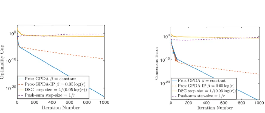
Figure 2.3: Results for the matrix factorization problem.
0 1000 2000 3000 4000 5000 Iteration number 10-8 10-6 10-4 10-2 100 102 104 O p ti m al it y G ap Prox-PDA-IP EXTRA-AO 0 1000 2000 3000 4000 5000 Iteration Number 10-10 10-5 100 105 1010 C o n s e n s u s E r r o r Prox-PDA-IP EXTRA-AO
Figure 2.4: Results for the matrix factorization problem.
2.7 Numerical Results
In this section, we demonstrate the performance of the proposed algorithms. All experiments are performed in Matlab (2016b) on a laptop with an Intel Core(TM) i5-4690 CPU (3.50 GHz) and 8GB RAM running Windows 7.
2.7.1 Distributed Binary Classification
In this subsection, we study the problem of binary classification using nonconvex regularizers in the mini-bach setup i.e. each node stores b(batch size) data points, and each component function is given by fi(xi) = 1 N b b X j=1
log(1 + exp(−yjxTi vj)) + M X k=1 λαx2i,k 1 +αx2i,k
where vi ∈ RM and yi ∈ {1,−1} are the feature vector and the label for the ith date point [7].
We use the parameter settings of λ= 0.001, α= 1 and M = 10. We randomly generated 100,000 data points and distribute them into N = 20 nodes (i.e. b = 5000). We use the optimality gap (opt-gap) and constraint violation (con-vio), displayed below, to measure the quality of the solution generated by different algorithms:
opt-gap := N X i=1 ∇fi(zi) 2
+kAxk2, con-vio =kAxk2.
We compare the the Prox-GPDA, and Prox-GPDA-IP with the distributed subgradient (DSG) method [100] (which is only known to work for convex cases) and the Push-sum algorithm [131]. The performance of all three algorithms in terms of the consensus error and the optimality gap (averaged over 30 problem instances) are presented in Fig. 2.3. The penalty parameter for Prox-GPDA is chosen such that satisfies (2.14), and βr for Prox-GPDA-IP is set as 0.05 log(r), the stepsizes of the DSG algorithm and the Push-sum algorithm are chosen as 1/0.05 log(r) and 1/r, respectively. Note that these parameters are tuned for each algorithm to achieve the best results. It can be observed that the Prox-GPDA with constant stepsize outperforms other algorithms. The Push-sum algorithm does not seem to converge within 1000 iterations.
2.7.2 Distributed Matrix Factorization
In this section we consider the distributed matrix factorization problem (2.26). The training data is constructed by randomly extracting 300 overlapping patches from the 512×512 image of barbara.png, each with size 16×16 pixels. Each of the extracted patch is vectorized, resulting a training data setZ of size 256×300. We consider a network ofN = 10 agents, and the columns ofZ
are evenly distributed among the agents (each havingP = 30 columns). We compare Prox-PDA-IP (a variant of Prox-PDA with increasing stepsize) with the EXTRA-AO algorithm proposed in [52]. Note that the EXTRA-AO is also designed for a similar distributed matrix factorization problem and it works well in practice. However, it does not have formal convergence proof. We initialize both algorithms with X being the 2D discrete cosine transform (DCT) matrix. We set γ = 0.05,
τ = 105 and β = 0.001r, and the results are averaged over 10 problem instances. The stepsizes of the EXTRA-AO is set asαAO= 0.03 and βAO= 0.002.
In Fig. 2.4, we compare the performance of the proposed Prox-PDA-IP and the EXTRA-AO versus the number of iterations. It can be observed that our proposed algorithm converges faster than the EXTRA-AO. We have observed that the EXTRA-AO does have reasonably good practical performance, however it lacks formal convergence proof.
2.8 Appendix. Lemma proofs 2.8.1 Proof of Lemma 23
From the optimality condition of the x problem (4.12a) we have
∇f(xr+1) +AT(µr+βAxr+1) +βBTB(xr+1−xr) = 0.
Applying (2.7b), we have
ATµr+1=−∇f(xr+1)−βBTB(xr+1−xr). (2.33) From equation (2.7b) (µr+1=µr+βATµr) it is clear the difference of the dual variables lies in the column space of A. Therefore the following is true
σmin1/2kµr+1−µrk ≤ kAT(µr+1−µr)k.
This inequality combined with (2.33) implies that
kµr+1−µrk ≤ 1 σmin1/2 k − ∇f(xr+1)−βBTB(xr+1−xr)−(−∇f(xr)−βBTB(xr−xr−1))k = 1 σmin1/2 ∇f(xr)− ∇f(xr+1)−βBTBwr .
Squaring both sides and dividing byβ, we obtain the desired result. Q.E.D.
2.8.2 Proof of Lemma 2
Sincef(x) has Lipschitz continuous gradient, and thatATA+BTB I by Assumption [A1], it is known that ifβ > L, then thex-problem (4.12a) is strongly convex with modulusγ :=β−L >0;
See [150] [Theorem 2.1]. That is, we have Lβ(x, µr) + β 2kx−x rk2 BTB−(Lβ(z, µr) + β 2kz−x rk2 BTB) ≥ h∇xLβ(z, µr) +β(BTB(z−xr)), x−zi+ γ 2kx−zk 2, ∀x, z ∈ RN, ∀µr. (2.34)
Using this property, we have
Lβ(xr+1, µr+1)−Lβ(xr, µr) =Lβ(xr+1, µr+1)−Lβ(xr+1, µr) +Lβ(xr+1, µr)−Lβ(xr, µr) ≤Lβ(xr+1, µr+1)−Lβ(xr+1, µr) +Lβ(xr+1, µr) + β 2kx r+1−xrk2 BTB−Lβ(xr, µr) (i) ≤ kµ r+1−µrk2 β +h∇xLβ(x r+1, µr) +β(BTB(xr+1−xr)), xr+1−xri − γ 2kx r+1−xrk2 (ii) ≤ kµ r+1−µrk2 β − γ 2kx r+1−xrk2 ≤ 1 σmin 2L2 β xr−xr+1 2 + 2βBTBwr 2 −γ 2kx r+1−xrk2 =− β−L 2 − 2L2 βσmin kxr+1−xrk2+ 2β σmin BTBwr 2 (2.35)
where in (i) we have used (2.34) with the identification z=xr+1 and x=xr and the fact that
Lβ(xr+1, µr+1)−Lβ(xr+1, µr) =hµr+1−µr, Axr+1i=
1
βkµ
r+1−µrk2
; in (ii) we have used the optimality condition for the x-subproblem (4.12a). The claim is proved. Q.E.D.
2.8.3 Proof of Lemma 3
From the optimality condition of the x-subproblem (4.12a) we have
h∇f(xr+1) +ATµr+βATAxr+1+βBTB(xr+1−xr), xr+1−xi ≤0, ∀ x∈RQ.
If we shiftr tor−1, we get
Plugging x = xr into the first inequality and x = xr+1 into the second, adding the resulting inequalities and utilizing the µ-update step (2.7b) we obtain
h∇f(xr+1)− ∇f(xr) +AT(µr+1−µr) +βBTBwr, xr+1−xri ≤0.
Rearranging, we have
hAT(µr+1−µr), xr+1−xri ≤ −h∇f(xr+1)− ∇f(xr) +βBTBwr, xr+1−xri. (2.36)
Let us bound the lhs and the rhs of (2.36) separately. First the lhs of (2.36) can be expressed as
hAT(µr+1−µr), xr+1−xri=hβATAxr+1, xr+1−xri =hβAxr+1, Axr+1−Axri =βkAxr+1k2−βhAxr+1, Axri = β 2 kAx r+1k2− kAxrk2+kA(xr+1−xr)k2 . (2.37)
Second we have the following bound for the rhs of (2.36)
− h∇f(xr+1)− ∇f(xr) +βBTBwr, xr+1−xri ≤Lkxr+1−xrk2−βhBTBwr, xr+1−xri =Lkxr+1−xrk2+β 2 kxr−xr−1k2BTB− kxr+1−xrk2BTB− kwrk2BTB . (2.38)
Combining the above two bounds, we have
β 2 kAx r+1k2+kxr+1−xrk2 BTB ≤Lkxr+1−xrk2+β 2 kx r−xr−1k2 BTB+kAxrk2 −β 2 kw rk2 BTB+kA(xr+1−xr)k2 .
2.8.4 Proof of Lemma 4
Multiplying both sides of (2.10) by the constantc and then add them to (2.9), we obtain
Lβ(xr+1, µr+1) + cβ 2 kAx r+1k2+kxr+1−xrk2 BTB ≤Lβ(xr, µr) +cLkxr+1−xrk2+ cβ 2 kx r−xr−1k2 BTB+kAxrk2 − β−L 2 − 2L2 βσmin kxr+1−xrk2+ 2β σmin BTBwr 2 −cβ 2 kw rk2 BTB+kA(xr+1−xr)k2 ≤Lβ(xr, µr) + cβ 2 kx r−xr−1k2 BTB+kAxrk2 − β−L 2 − 2L2 βσmin −cL kxr+1−xrk2− cβ 2 − 2βkBTBk F σmin kwrk2BTB.
The desired result is proved. Q.E.D.
2.8.5 Proof of Lemma 25
To prove this we need to utilize the boundedness assumption in [A2]. First, we can express the augmented Lagrangian function as following
Lβ(xr+1, µr+1) =f(xr+1) +hµr+1, Axr+1i+ β 2kAx r+1k2 =f(xr+1) + 1 βhµ r+1, µr+1−µri+β 2kAx r+1k2 =f(xr+1) + 1 2β kµ r+1k2− kµrk2+kµr+1−µrk2 +β 2kAx r+1k2.
Therefore, summing over r= 1· · · , T, we obtain
T X r=1 Lβ(xr+1, µr+1) = T X r=1 f(xr+1) +β 2kAx r+1k2+ 1 2βkµ r+1−µrk2 + 1 2β kµ T+1k2− kµ1k2 .
Suppose Assumption [A2] is satisfied and β is chosen according to (2.13) and (2.14), then clearly the above sum is lower bounded since
f(x) + β 2kAxk 2≥f(x) +δ 2kAxk 2 ≥0, ∀ x∈ RQ.
This fact implies that the sum of the potential function is also lower bounded (note, the remaining terms in the potential function are all nonnegative), that is
T
X
r=1
Note that if c and β are chosen according to (2.13) and (2.14), then Pc,β(xr+1, xr, µr+1) is
non-increasing. Combined with the lower boundedness of the sum of the potential function, we can conclude that the following is true
Pc,β(xr+1, xr, µr+1)>−∞, ∀ r >0. (2.39)
This completes the proof. Q.E.D.
2.8.6 Proof of Theorm 1
First we prove part (1). Combining Lemmas 4 and 25, we conclude that kxr+1−xrk2 → 0. Then according to (5.32), in the limit we have µr+1 →µr, or equivalently Axr → 0. That is, the
constraint violation will be satisfied in the limit.
Then we prove part (2). From the optimality condition of x-update step (4.12a) we have
∇f(xr+1) +ATµr+βAT(Axr+1) +βBTB(xr+1−xr) = 0.
Then we argue that {µr} is a bounded sequence if ∇f(xr+1) is bounded. Indeed the fact that
kxr+1−xrk2 →0 andAxr+1→0 imply that both (xr+1−xr) and Axr+1 are bounded. Then the boundedness of µr follows from the assumption that ∇f(x) is bounded for any x∈ RQ, and that
µr lies in the column space ofA.
Then we argue that {xr} is bounded if f(x) + β
2kAxk
2 is coercive. Note that the potential function can be expressed as
Pc,β(xr+1, xr, µr+1) =f(xr+1) +hµr+1, Axr+1i+ β 2kAx r+1k2+ cβ 2 kAx r+1k2+kxr+1−xrk2 BTB =f(xr+1) + 1 2β(kµ r+1k2− kµrk2+kµr+1−µrk2) +β 2kAx r+1k2 +cβ 2 kAx r+1k2+kxr+1−xrk2 BTB
and by our analysis in Lemma 25we know that it is decreasing thus upper bounded. Suppose that
{xr} is unbounded and let K denote an infinite subset of iteration index in which lim
r∈Kxr =∞. Passing limit toPc,β(xr+1, xr, µr+1) overK, and using the fact thatxr+1 →xr,µr+1 →µr, we have
lim r∈K Pc,β(xr+1, xr, µr+1) = lim r∈K f(xr+1) +cβ+β 2 kAx r+1k=∞
![Figure 4.1: Comparison of proposed algorithms with DSG [102] and NEXT [92] in terms of sta-tionary gap for problem 4.114 with parameters N = 20, R = 0.7, d = 10, α = 0.01](https://thumb-us.123doks.com/thumbv2/123dok_us/385053.2542668/139.918.523.749.224.402/figure-comparison-proposed-algorithms-terms-tionary-problem-parameters.webp)