Runtime Optimizations for Tree-based
Machine Learning Models
Nima Asadi, Jimmy Lin, and Arjen P. de Vries
Abstract—Tree-based models have proven to be an effective solution for web ranking as well as other machine learning problems in diverse domains. This paper focuses on optimizing the runtime performance of applying such models to make predictions, specifically using gradient-boosted regression trees for learning to rank. Although exceedingly simple conceptually, most implementations of tree-based models do not efficiently utilize modern superscalar processors. By laying out data structures in memory in a more cache-conscious fashion, removing branches from the execution flow using a technique called predication, and micro-batching predictions using a technique called vectorization, we are able to better exploit modern processor architectures. Experiments on synthetic data and on three standard learning-to-rank datasets show that our approach is significantly faster than standard implementations.
Index Terms—Web search, general information storage and retrieval, information technology and systems, scalability and efficiency, learning to rank, regression trees
1
I
NTRODUCTIONR
ECENT studies have shown that machine-learned tree-based models, combined with ensemble tech-niques, are highly effective for building web ranking algo-rithms [1]–[3] within the “learning to rank” framework [4]. Beyond document retrieval, tree-based models have also been proven effective for tackling problems in diverse domains such as online advertising [5], medical diagno-sis [6], genomic analysis [7], and computer vision [8]. This paper focuses on runtime optimizations of tree-based mod-els that take advantage of modern processor architectures: we assume that a model has already been trained, and now we wish to make predictions on new data as quickly as pos-sible. Although exceedingly simple, standard implementa-tions of tree-based models do not efficiently utilize modern processor architectures due to the prodigious amount of branches and non-local memory references. By laying out data structures in memory in a more cache-conscious fash-ion, removing branches from the execution flow using a technique called predication, and micro-batching predic-tions using a technique called vectorization, we are able to better exploit modern processor architectures and sig-nificantly improve the speed of tree-based models over hard-coded if-else blocks and alternative implementations.• N. Asadi is with the Department of Computer Science, University of Maryland, College Park, MD 20742 USA. E-mail:[email protected].
• J. Lin is with the College of Information Studies, University of Maryland, College Park, MD 20742 USA. E-mail:[email protected].
• A. P. de Vries is with the Centrum Wiskunde and Informatica (CWI), Amsterdam 1098 XG, Netherlands. E-mail:[email protected].
Manuscript received 18 July 2012; revised 18 Apr. 2013; accepted 19 Apr. 2013. Date of publication 2 May 2013; date of current version 31 July 2014. Recommended for acceptance by B. Cooper.
For information on obtaining reprints of this article, please send e-mail to:
[email protected], and reference the Digital Object Identifier below. Digital Object Identifier 10.1109/TKDE.2013.73
Our experimental results are measured in nanoseconds for individual trees and microseconds for complete ensem-bles. A natural starting question is: do such low-level optimizations actually matter? Does shaving microseconds off an algorithm have substantive impact on a real-world task? We argue that the answer is yes, with two different motivating examples: First, in our primary application of learning to rank for web search, prediction by tree-based models forms the inner loop of a search engine. Since commercial search engines receive billions of queries per day, improving this tight inner loop (executed many bil-lions of times) can have a noticeable effect on the bottom line. Faster prediction translates into fewer servers for the same query load, reducing datacenter footprint, electricity and cooling costs, etc. Second, in the domain of financial engineering, every nanosecond counts in high frequency trading. Orders on NASDAQ are fulfilled in less than 40 microseconds.1Firms fight over the length of cables due to speed-of-light propagation delays, both within an individ-ual datacenter and across oceans [9].2 Thus, for machine learning in financial engineering, models that shave even a few microseconds off prediction times present an edge.
The contribution of this work lies in novel imple-mentations of tree-based models that are highly-tuned to modern processor architectures, taking advantage of cache hierarchies and superscalar processors. We illustrate our techniques on three separate learning-to-rank datasets and show significant performance improvements over standard implementations. Although our interest lies primarily in machine learning for web search ranking, there is noth-ing in this paper that is domain-specific. To the extent that tree-based models represent effective solutions, we expect
1.http://www.nasdaqtrader.com/Trader.aspx?id=colo 2. http://spectrum.ieee.org/computing/it/financial-trading-at-the-speed-of-light
1041-4347 c2013 IEEE. Personal use is permitted, but republication/redistribution requires IEEE permission. See http://www.ieee.org/publications_standards/publications/rights/index.html for more information.
our results to generalize to machine learning applications in other domains.
More generally, our work enriches the literature on
architecture-conscious optimizations for machine learning
algorithms. Although database researchers have long real-ized the importance of designing algorithms that match the characteristics of processor architectures [10]–[14], this topic has not received much attention by the information retrieval, machine learning, and data mining communities. Although we are not the first to examine the problem of architecture-conscious algorithms for machine learning, the literature is sparsely populated and we contribute to the field’s understanding of performance optimizations for an important class of applications.
2
B
ACKGROUND ANDR
ELATEDW
ORK2.1 Processor Architectures
We begin with an overview of modern processor architec-tures and recap advances over the past few decades. The broadest trend is perhaps the multi-core revolution [15]: the relentless march of Moore’s Law continues to increase the number of transistors on a chip exponentially, but com-puter architects widely agree that we are long past the point of diminishing returns in extracting instruction-level par-allelism in hardware. Instead, adding more cores appears to be a better use of increased transistor density. Since prediction is an embarrassingly parallel problem, our tech-niques can ride the wave of increasing core counts (but see discussion in Section6).
A less-discussed, but just as important trend over the past two decades is the so-called “memory wall” [14], where increases in processor speed have far outpaced decreases in memory latency. This means that, relatively, RAM is becoming slower. In the 1980s, memory latencies were on the order of a few clock cycles; today, it could be several hundred clock cycles. To hide this latency, computer architects have introduced hierarchical cache memories: a typical server today will have L1, L2, and L3 caches between the processor and main memory. Cache architec-tures are built on the assumption of reference locality—that at any given time, the processor repeatedly accesses only a (relatively) small amount of data, and these fit into cache. The fraction of memory accesses that can be ful-filled directly from the cache is called the cache hit rate, and data not found in cache are said to cause a cache miss. Cache misses cascade down the hierarchy—if a datum is not found in L1, the processor tries to look for it in L2, then in L3, and finally in main memory (paying an increasing latency cost each level down).
Managing cache content is a complex challenge, but there are two main principles that are relevant for a soft-ware developer. First, caches are organized into cache lines (typically 64 bytes), which is the smallest unit of transfer between cache levels. That is, when a program accesses a particular memory location, the entire cache line is brought into (L1) cache. This means that subsequent references to nearby memory locations are very fast, i.e., a cache hit. Therefore, in software it is worthwhile to organize data structures to take advantage of this fact. Second, if a program accesses memory in a predictable sequential
pattern (called striding), the processor will prefetch mem-ory blocks and move them into cache, before the program has explicitly requested them (and in certain architectures, it is possible to explicitly control prefetch in software). There is, of course, much more complexity beyond this short description; see [16] for an overview.
Another salient property of modern CPUs is pipelining, where instruction execution is split between several stages (modern processors have between one and two dozen stages). At each clock cycle, all instructions “in flight” advance one stage in the pipeline; new instructions enter the pipeline and instructions that leave the pipeline are “retired”. Pipeline stages allow faster clock rates since there is less to do per stage. Modern superscalar CPUs add the ability to dispatch multiple instructions per clock cycle (and out of order) provided that they are independent.
Pipelining suffers from two dangers, known as “haz-ards” in VLSI design terminology. Data hazards occur when one instruction requires the result of another (that is, a data dependency). This happens frequently when derefer-encing pointers, where we must first compute the memory location to access. Subsequent instructions cannot pro-ceed until we actually know what memory address we are requesting—the processor simply stalls waiting for the result (unless there is another independent instruction that can be executed). Control hazards are instruction depen-dencies introduced by if-then clauses (which compile to conditional jumps in assembly). To cope with this, modern processors use branch prediction techniques—in short, try-ing to predict which code path will be taken. However, if the guess is not correct, the processor must “undo” the instructions that occurred after the branch point (“flushing” the pipeline). With trees, one would naturally expect many branch mispredicts.
The database community has explored in depth the con-sequences of modern processor architectures for relational data processing [10]–[14]. For example, researchers discov-ered over a decade ago that data and control hazards can have a substantial impact on performance: an influen-tial paper in 1999 concluded that in commercial RDBMSes at the time, almost half of the execution time was spent on stalls [10]. Since then, researchers have productively tackled this and related issues by designing architecture-conscious algorithms for relational data processing. In con-trast, this topic has not received much attention by the information retrieval, machine learning, and data mining communities.
The two optimization techniques central to our approach borrow from previous work. Using a technique called pred-ication [17], [18], originally from compilers, we can convert control dependencies into data dependencies. However, as compiler researchers know well, predication does not always help—under what circumstances it is worthwhile for our machine learning application is an empirical ques-tion we examine.
Another optimization that we adopt, vectorization, was pioneered by database researchers [13], [19]: the basic idea is that instead of processing a tuple at a time, a relational query engine should process a vector (i.e., batch) of tuples at a time to take advantage of pipelining and to mask memory latencies. We apply this idea to prediction with
tree-based models and are able to obtain many of the same benefits.
Although there is much work on scaling the training of tree-based models to massive datasets [5], [20], it is orthogonal to the focus of this paper, which is architecture-conscious runtime optimizations. We are aware of a few papers that have explored this topic. Ulmer et al. [21] described techniques for accelerating text-similarity clas-sifiers using FPGAs. Sharp [22] explored decision tree implementations on GPUs for image processing applica-tions. Other than the obvious GPU vs. CPU differences: although his approach also takes advantage of predication, we describe a slightly more optimized implementation. Similarly, Essen et al. [23] compared multi-core, GPU, and FPGA implementations of compact random forests. They also take advantage of predication, but there are minor dif-ferences that make our implementation more optimized. Furthermore, neither of these two papers take advantage of vectorization, although it is unclear how vectorization applies to GPUs, since they are organized using very dif-ferent architectural principles. We will detail the differences between these and our implementations in Section3.
2.2 Learning to Rank and LambdaMART
The particular problem we focus on in this paper is learn-ing to rank—the application of machine learnlearn-ing techniques to document ranking in text retrieval. Following the stan-dard formulation [4], we are given a document collection
D and a training set S= {(xi,yi)}mi=1, where xi is an input feature vector and yi is a relevance label (in the simplest case, relevant or not-relevant, but more commonly, labels drawn from a graded relevance scale). Each input feature vector xi is created from φ(qi,di,j), where qi represents a sample query and di,1. . .di,jrepresent documents for which we have some relevance information, on which the fea-ture function φ is applied to extract features. Given this, the learning to rank task is to induce a function f(q,D)
that assigns scores to query–document pairs (or equiva-lently, feature vectors) such that the ranking induced by the document scores maximizes a metric such as NDCG [24].
Our work takes advantage of gradient-boosted regres-sion trees (GBRTs) [1]–[3], [25], a state-of-the-art ensemble method. Specifically, we use LambdaMART [1], which is the combination of LambdaRank [26] and MART [27], a class of boosting algorithms that performs gradient descent using regression trees.
LambdaMART learns a ranking model by sequentially adding new trees to an ensemble that best account for the remaining regression error (i.e., the residuals) of the training samples. More specifically, LambdaMART learns a linear predictor Hβ(x)=βh(x)that minimizes a given loss function(Hβ), where the base learners are limited-depth regression trees [28]: h(x)=[h1(x), . . . ,hT(x)], where ht∈H, andHis the set of all possible regression trees.
Assuming we have constructed t−1 regression trees in the ensemble, LambdaMART adds the t-th tree that greedily minimizes the loss function, given the current pseudo-responses. CART [28] is used to generate a regression tree with J terminal nodes, which works by recursively split-ting the training data. At each step, CART computes the best split (a feature and a threshold) for all terminal nodes,
and then applies the split that results in the highest gain, thereby growing the tree one node at a time. Consider the following cost function:
C(N,f, θN)= xi∈L (yi− ¯yL)2+ xi∈R (yi− ¯yR)2, (1) where L and R are the left and right sets containing the instances that fall to the left and right of node N after the split is applied, respectively; N denotes a node in the tree; f, θN is a pair consisting of a feature and a threshold; xi and yi denote an instance and its associated pseudo-response. Minimizing Equation (1) is equivalent to maximizing the difference in C(·) before and after a split is applied to node N. This difference can be computed as follows:
G(N,f, θN)=
xi∈N
(yi− ¯yN)2−C(N,f, θN), (2) where xi ∈N denotes the set of instances that are present
in node N.
The final LambdaMART model has low bias but is prone to overfitting the training data (i.e., model has a high variance). In order to reduce the variance of an ensem-ble model, bagging [29] and randomization can be utilized during the training. Friedman [27] introduces the following randomization techniques:
• A weak learner is fit on a sub-sample of the training set drawn at random without replacement.
• Similar to Random Forests [30], to determine the best tree split, the algorithm picks the best feature from a random subset of all features (as opposed to choosing the best overall feature).
Ganjisaffar et al. [2] take randomization one step further and construct multiple ensembles, each built using a random bootstrap of the training data (i.e., bagging multiple boosted ensembles). In this work, we limit our experiments to the two randomization techniques discussed above and do not explore bagging the boosted ensembles—primarily because bagging is embarrassingly-parallel from the runtime execu-tion perspective and hence not particularly interesting.
Related to our work, there is an emerging thread of research, dubbed “learning to efficiently rank”, whose goal is to train models that deliver both high-quality results and are fast in ranking documents [31]–[33]. For exam-ple, Wang et al. [32] explored a cascade of linear rankers and Xu et al. [33] focused on training tree-based models that minimize feature-extraction costs. This line of research is complementary to our work since it focuses on training models that better balance effectiveness and efficiency; in contrast, we develop optimizations for executing tree-based models. In other words, our techniques can provide the execution framework for models delivered by Xu et al.
A final piece of relevant work is that of Cambazoglu
et al. [34]: in the context of additive ensembles (of which boosted trees are an example) for learning to rank, they explored early-exit optimizations for top k ranking. The authors empirically showed that, using a number of heuris-tics, it is possible to skip evaluation of many stages in an ensemble (thereby increasing the performance of the ranker) with only minimal loss in result quality. While
this approach has the same overall goals as our work, it is orthogonal since we are focusing on a different aspect of the problem—efficient execution of the individual tree-based models that comprise an additive ensemble. There is no reason why the optimizations of Cambazoglu et al. [34] cannot be applied on top of our work. Finally, we note that our optimizations are more general, since their work is only applicable to top k retrieval problems and sacrifices some quality.
3
T
REEI
MPLEMENTATIONSIn this section, we describe various implementations of tree-based models, progressively introducing architecture-conscious optimizations. We focus on an individual tree, the runtime execution of which involves checking a predicate in an interior node, following the left or right branch depend-ing on the result of the predicate, and repeatdepend-ing until a leaf node is reached. We assume that the predicate at each node involves a feature and a threshold: if the feature value is less than the threshold, the left branch is taken; other-wise, the right branch is taken. Of course, trees with greater branching factors and more complex predicate checks can be converted into an equivalent binary tree, so our formula-tion is entirely general. Note that our discussion is agnostic with respect to the prediction at the leaf node.
We assume that the input feature vector is densely-packed in a floating-point array (as opposed to a sparse, map-based representation). This means that checking the predicate at each tree node is simply an array access, based on a unique consecutively-numbered id associated with each feature.
OBJECT: As a naïve baseline, we consider an implemen-tation of trees with nodes and associated left and right pointers in C++. Each tree node is represented by an object, and contains the feature id to be examined as well as the decision threshold. For convenience, we refer to this as the OBJECT implementation.
This implementation has two advantages: simplicity and flexibility. However, we have no control over the physical layout of the tree nodes in memory, and hence no guaran-tee that the data structures exhibit good reference locality. Prediction with this implementation essentially boils down to pointer chasing across the heap: when following either the left or the right pointer to the next tree node, the processor is likely to be stalled by a cache miss.
STRUCT: The OBJECT approach has two downsides: poor memory layout (i.e., no reference locality and hence cache misses) and rather inefficient memory utilization (due to object overhead). To address the second point, the solu-tion is to avoid objects and implement each node as a
struct (comprising feature id, threshold, left and right
pointers). We construct a tree by allocating memory for each node (malloc) and assigning the pointers appropriately. Prediction with this implementation remains an exercise in pointer chasing, but now across much more memory-efficient data structures. We refer to this as the STRUCT
implementation.
STRUCT+: An improvement over the STRUCT implementa-tion is to physically manage the memory layout ourselves.
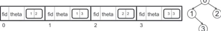
Fig. 1. Memory layout of the PREDimplementation for a sample tree. Instead of allocating memory for each node individually, we allocate memory for all the nodes at once (i.e., an array
of structs) and linearize the order of the nodes via a
breadth-first traversal of the tree, with the root at index 0. The STRUCT+ implementation occupies the same amount of memory as STRUCT, except that the memory is contiguous. The hope is that by manually controlling mem-ory layout, we can achieve better reference locality, thereby speeding up memory references. This is similar to the idea behind CSS-Trees [11] used in the database community. For convenience we call this the STRUCT+ implementation. CODEGEN: Next, we consider statically-generated if-else blocks. A code generator takes a tree model and directly generates C code, which is then compiled and used to make predictions. For convenience, we refer to this as the CODEGENimplementation.
We expect this approach to be fast. The entire model is statically specified; machines instructions are expected to be relatively compact and will fit into the processor’s instruction cache, thus exhibiting good reference locality. Furthermore, we leverage decades of compiler optimiza-tions that have been built intogcc. Note that this eliminates data dependencies completely by converting them all into control dependencies.
PRED: The STRUCT+ implementation tackles the reference locality problem, but there remains the presence of branches (resulting from the conditionals), which can be quite expen-sive to execute. The CODEGENimplementation suffers from this drawback as well. Branch mispredicts cause pipeline stalls and wasted cycles (and of course, we would expect many mispredicts with trees). Although it is true that spec-ulative execution renders the situation far more complex, removing branches may yield performance increases. A well-known trick in the compiler community for overcom-ing these issues is known as predication [17], [18]. The underlying idea is to convert control dependencies (haz-ards) into data dependencies (haz(haz-ards), thus altogether avoiding jumps in the underlying assembly code.
Here is how predication is adapted for our case: We encode the tree as a struct array in C, nd, where
nd[i].fidis the feature id to examine andnd[i].theta
is the threshold. The nodes are laid out via breadth-first traversal of the tree. Each node, regardless of being interme-diate or terminal, additionally holds an array of two inte-gers. The first integer field holds the index of the left child in the array representation, and the second integer holds that of the right child. We use self loops to connect every leaf to itself (more below). A sample memory structure of nodes in the proposed implementation is illustrated in Fig.1.
To make the prediction, we probe the array in the following manner:
i = nd[i].index[(v[nd[i].fid] >= nd[i].theta)]; i = nd[i].index[(v[nd[i].fid] >= nd[i].theta)];
That is, if the condition holds, we visit the right node (index 1 of the index array); otherwise, we visit the left node (index 0 of the index array). In case we reach a leaf before the
d-th statement, we would be sent back to the same node
regardless of the condition by the self loops.
We completely unroll the tree traversal loop, so the above statement is repeated d times for a tree of depth
d. At the end, i contains the index of the leaf node
cor-responding to the prediction (which we look up in another array). Note that the self loops allow us to represent unbal-anced trees without introducing additional complexity into the tree traversal logic. Since there is no need to check if we have reached the leaf, we can safely unroll the entire loop without affecting the correctness of the algorithm. One final implementation detail: we hard code a prediction function for each tree depth, and then dispatch dynamically using function pointers.
Although the basic idea of using predication to opti-mize tree execution is not novel, there are a few minor differences between our implementation and those from previous work that may have substantial impact on per-formance. For example, the GPU implementation of tree models by Sharp [22] takes advantage of predication and loop unrolling, but in order to handle unbalanced trees each node must store a flag indicating whether or not it is a leaf node. Tree traversal requires checking this flag at each node, which translates into an additional conditional branch at each level in the tree. We avoid this additional comparison by the “self loop” trick described above: note that these self loops have minimal impact on performance, since they are accessing data structures that have already been loaded into cache. In another example, the work of Essen et al. [23] also take advantage of predication, but their implementation also requires this additional leaf node check; furthermore, they do not unroll their loops, which introduces additional branch instructions (and branch mispredicts upon exiting loops).
VPRED: Predication eliminates branches but at the cost of introducing data hazards. Each statement in PREDrequires an indirect memory reference. Subsequent instructions can-not execute until the contents of the memory location are fetched—in other words, the processor will simply stall waiting for memory references to resolve. Therefore, predi-cation is entirely bottlenecked on memory access latencies. A common technique adopted in the database literature to mask these memory latencies is called vectorization [13], [19]. Applied to our task, this translates into operating on multiple instances (feature vectors) at once, in an inter-leaved way. This takes advantage of multiple dispatch and pipelining in modern processors (provided that there are no dependencies between dispatched instructions, which is true in our case). Thus, while the processor is waiting for the memory access from the predication step on the first instance, it can start working on the second instance. In fact, we can work on v instances in parallel. For v=4, this looks like the following, processing instances i0,i1, i2,
i3in parallel: i0 = nd[i0].index[(v[nd[i0].fid] >= nd[i0].theta)]; i1 = nd[i1].index[(v[nd[i1].fid] >= nd[i1].theta)]; i2 = nd[i2].index[(v[nd[i2].fid] >= nd[i2].theta)]; i3 = nd[i3].index[(v[nd[i3].fid] >= nd[i3].theta)]; i0 = nd[i0].index[(v[nd[i0].fid] >= nd[i0].theta)]; i1 = nd[i1].index[(v[nd[i1].fid] >= nd[i1].theta)]; i2 = nd[i2].index[(v[nd[i2].fid] >= nd[i2].theta)]; i3 = nd[i3].index[(v[nd[i3].fid] >= nd[i3].theta)]; ...
In other words, we traverse one layer in the tree for four instances at once. While we’re waiting for
v[nd[i0].fid] to resolve, we dispatch instructions for
accessing v[nd[i1].fid], and so on. Hopefully, by the time the final memory access has been dispatched, the con-tents of the first memory access are available, and we can continue without processor stalls. In this manner, we expect vectorization to mask memory latencies.
Again, we completely unroll the tree traversal loop, so each block of statements is repeated d times for a tree of depth d. At the end, the i’s contain the indexes of the leaf nodes corresponding to the prediction for the v instances. Setting v to 1 reduces this model to pure predi-cation (i.e., no vectorization). Note that the optimal value of v is dependent on the relationship between the amount of computation performed and memory latencies—we will determine this relationship empirically. For convenience, we refer to the vectorized version of the predication tech-nique as VPRED.
Note that previous work on optimizing tree-based mod-els using predication [22], [23] does not take advantage of vectorization. However, in fairness, it is unclear to what extent vectorization is applicable in the GPU execu-tion environment explored in the cited work, since GPUs support parallelism through a large number of physical processing units.
4
E
XPERIMENTALS
ETUPGiven that the focus of our work is efficiency, our primary evaluation metric is prediction speed, measured in terms of latency. We define this as the elapsed time between the moment a feature vector (i.e., a test instance) is presented to the tree-based model to the moment that a prediction is made for the instance (in our case, a regression value). To increase the reliability of our results, we conducted multiple trials, reporting the averages as well as the 95% confidence intervals.
We conducted two sets of experiments: first, using syn-thetically-generated data to quantify the performance of individual trees in isolation, and second, on standard learning-to-rank datasets to verify the end-to-end perfor-mance of full ensembles.
All experiments were run on a Red Hat Linux server, with Intel Xeon Westmere quad-core processors (E5620 2.4GHz). This architecture has a 64KB L1 cache per core, split between data and instructions; a 256KB L2 cache per core; and a 12MB L3 cache shared by all cores. Code was compiled with GCC (version 4.1.2) using opti-mization flags -O3 -fomit-frame-pointer -pipe. In our main experiments, all code ran single-threaded, but we report on multi-threaded experiments in Section6. In order to facilitate the reproducibility of these results and so that others can build on our work, all code neces-sary to replicate these experiments are made available at
4.1 Synthetic Data
The synthetic data consist of randomly generated trees and randomly generated feature vectors. Each intermediate node in a tree has two fields: a feature id and a thresh-old on which the decision is made. Each leaf is associated with a regression value. Construction of a random tree of depth d begins with the root node. We pick a feature id at random and generate a random threshold to split the tree into left and right subtrees. This process is recursively per-formed to build each subtree until we reach the desired tree depth. When we reach a leaf node, we generate a regression value at random. Note that our randomly-generated trees are fully-balanced, i.e., a tree of depth d has 2d leaf nodes. Once a tree has been constructed, the next step is to gen-erate random feature vectors. Each random feature vector is simply a floating-point array of length f (= number of features), where each index position corresponds to a fea-ture value. We assume that all paths in the decision tree are equally likely; the feature vectors are generated in a way that guarantees an equal likelihood of visiting each leaf. To accomplish this, we take one leaf at a time and follow its parents back to the root. At each node, we take the node’s feature id and produce a feature value based on the position of the child node. That is, if the child node we have just vis-ited is on the left subtree we generate a feature value that is smaller than the threshold stored at the current parent node and vice versa. We randomize the order of instances once we have generated all the feature vectors. To avoid any cache effects, experiments were conducted on a large number of instances (512K).
Given a random tree and a set of random feature vectors, we ran experiments to assess the various implementations of tree-based models described in Section3. To get a bet-ter sense of the variance, we performed five trials; in each trial we constructed a new random binary tree and a differ-ent randomly-generated set of feature vectors. To explore the design space, we conducted experiments with vary-ing tree depths d∈ {3,5,7,9,11}and varying feature sizes
f ∈ {32,128,512}. These feature values were selected based on actual learning-to-rank experiments (see below).
4.2 Learning-to-Rank Experiments
In addition to randomly-generated trees, we conducted experiments using standard learning-to-rank datasets. In these experiments, we are given training, validation, and test data as well as a tree-based learning-to-rank model. Using the training and validation sets we learn a com-plete tree ensemble. Evaluation is then carried out on test instances to determine the speed of the various algo-rithms. These end-to-end experiments give us insight on how different implementations compare in a real-world application.
We used three standard learning-to-rank datasets: LETOR-MQ2007,3 MSLR-WEB10K,4 and the Yahoo! Webscope Learning-to-Rank Challenge [35] dataset (C14 Set 1).5All three datasets are pre-folded, providing training,
3.http://research.microsoft.com/en-us/um/beijing/projects/ letor/letor4dataset.aspx
4.http://research.microsoft.com/en-us/projects/mslr/ 5.http://learningtorankchallenge.yahoo.com/datasets.php
TABLE 1
Average Number of Training, Validation, and Test Instances in Our Learning-to-Rank Datasets, along with the Number of
Features
validation, and test instances. Table1 shows the dataset size and the number of features. To measure variance, we repeated experiments on all folds. Note that MQ2007 is much smaller and contains a more impoverished feature set, considered by many in the community to be outdated. Further note that the C14 dataset only contains a single fold. The values of f (number of features) in our synthetic experiments are guided by these learning-to-rank datasets. We selected feature sizes that are multiples of 16 so that the feature vectors are integer multiples of cache line sizes (64 bytes): f =32 roughly corresponds to LETOR features and is representative of a small feature space; f =128 cor-responds to MSLR and is representative of a medium-sized feature space. Finally, the third condition f = 512 corre-sponds to the C14 dataset and captures a large feature space condition.
Our experiments used the open-source jforests imple-mentation6 of LambdaMART to optimize NDCG [24]. Although there is no way to precisely control the depth of each tree, we can adjust the size distribution of the trees by setting a cap on the number of leaves. To train an ensemble, we initialize the randomized LambdaMART algorithm with a random seed S. In order to capture the variance, we repeat this E=100 times for the LETOR and MSLR-WEB10K datasets and E = 20 times for the C14 dataset. We then repeat this procedure independently for each cross-validation fold. For LETOR and MSLR, we used the parameters of LambdaMART suggested by Ganjisaffar
et al. [2]: feature and data sub-sampling parameters (0.3), minimum observations per leaf (0.5), and the learning rate (0.05). We varied the max leaves parameter as part of our experimental runs. Note that Ganjisaffar et al. did not exper-iment with the C14 dataset, but we retained the same parameter settings (as above) for all except for the max leaves parameter.
5
R
ESULTSIn this section we present experimental results, first on synthetic data and then on learning-to-rank datasets.
5.1 Synthetic Data: Base Results
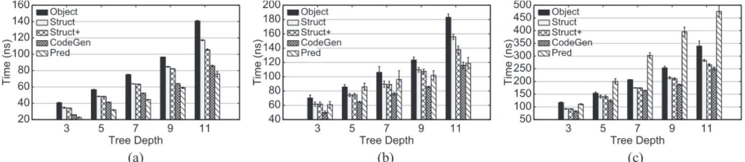
We begin by focusing on the first five implementations described in Section3 (leaving aside VPRED for now), using the procedure described in Section 4.1. The predic-tion time per randomly-generated test instance is shown in Fig. 2, measured in nanoseconds. The balanced randomly-generated trees vary in terms of tree depth d, and each bar chart shows a separate value of f (number of features). Time is averaged across five trials and error bars denote
(a) (b) (c)
Fig. 2. Prediction time per instance (in nanoseconds) on synthetic data using various implementations. Error bars denote 95% confidence intervals. (a) f = 32. (b) f = 128. (c) f = 512.
95% confidence intervals. It is clear that as trees become deeper, prediction speeds decrease overall. This is obvious since deeper trees require more feature accesses and pred-icate checks, more pointer chasing, and more branching (depending on the implementation).
First, consider the naïve and code-generation baselines. As expected, the OBJECT implementation is the slowest in most cases: this is no surprise due to object overhead. We can quantify this overhead by comparing the OBJECT
implementation with the STRUCT implementation, which replaces objects with lighter-weightstructs. As expected, the CODEGENimplementation is very fast: with the excep-tion of f = 32, hard-coded if-else blocks outperform all other implementations regardless of tree depth.
Comparing STRUCT+ with STRUCT, we observe no sig-nificant improvements for shallow trees, but sigsig-nificant speedups for deeper trees. Recall that in the first imple-mentation, we allocate memory for the entire tree so that it resides in a contiguous memory block, whereas in the sec-ond we let malloc allocate memory however it chooses. This shows that reference locality is important for deeper trees.
Finally, turning to the PREDcondition, we observe very interesting behavior. For small feature vectors f = 32, the technique is actually faster than even CODEGEN. This shows that for small feature sizes, predication helps to over-come branch mispredicts, i.e., converting control depen-dencies into data dependepen-dencies increases performance. For
f = 128, the performance of PRED is worse than that of CODEGEN (except for trees of depth 11). With the excep-tion of the deepest trees, PRED is about the same speed
as STRUCT and STRUCT+. For f = 512 (large feature vec-tors), the performance of PREDis terrible, even worse than the OBJECT implementation. We explain this result as fol-lows: PREDperformance is entirely dependent on memory access latency. When traversing the tree, it needs to wait for the contents of memory before proceeding. Until the memory references are resolved, the processor simply stalls. With small feature vectors, we get excellent locality: 32 fea-tures take up two 64-byte cache lines, which means that evaluation incurs at most two cache misses. Since mem-ory is fetched by cache lines, once a feature is accessed, accesses to all other features on the same cache line are essentially “free”. Locality decreases as the feature vector size increases: the probability that the predicate at a tree node accesses a feature close to one that has already been accessed goes down. Thus, as the feature vector size grows,
the PREDprediction time becomes increasingly dominated by stalls waiting for memory fetches.
The effect of this “memory wall” is evident in the other implementations as well. The performance differ-ences between CODEGEN, STRUCT, and STRUCT+ shrink as the feature size increases (whereas they are much more pronounced for smaller feature vectors). This is because as feature vector size increases, more and more of the prediction time is dominated by memory latencies.
How can we overcome these memory latencies? Instead of simply stalling while we wait for memory references to resolve, we can try to do other useful computation—this is exactly what vectorization is designed to accomplish.
5.2 Tuning the Vectorization Parameter
In Section3, we proposed vectorization of the predication technique in order to mask memory latencies. The idea is to work on v instances (feature vectors) at the same time, so that while the processor is waiting for memory access for one instance, useful computation can happen on another. This takes advantage of pipelining and multiple dispatch in modern superscalar processors.
The effectiveness of vectorization depends on the rela-tionship between time spent in actual computation and memory latencies. For example, if memory fetches take only one clock cycle, then vectorization cannot possibly help. The longer the memory latencies, the more we would expect vectorization (larger batch sizes) to help. However, beyond a certain point, once memory latencies are effec-tively masked by vectorization, we would expect larger values of v to have little impact. In fact, values that are too large start to become a bottleneck on memory bandwidth and cache size.
In Fig. 3, we show the impact of various batch sizes,
v ∈ {1,4,8,16,32,64}, for the different feature sizes. As a special case, when v is set to 1, we evaluate one instance at a time using predication. This reduces to the PRED implemen-tation. Latency is measured in nanoseconds and normalized by batch size (i.e., divided by v), so we report per-instance prediction time. For f = 32, v = 8 yields the best perfor-mance; for f = 128, v = 16 yields the best performance; for f =512, v= {16,32,64} all provide approximately the same level of performance. These results are exactly what we would expect: since memory latencies increase with larger feature sizes, a larger batch size is needed to mask the latencies.
(a) (b) (c)
Fig. 3. Prediction time per instance (in nanoseconds) on synthetic data using vectorized predication, for varying values of the batch size v . v=1 represents the PREDimplementation. (a) f = 32. (b) f = 128. (c) f = 512.
Interestingly, the gains from vectorization for f =128 in Fig. 2(b) are not consistent with the gains shown in Fig. 2(a) for f = 32 and Fig. 2(c) for f =512. We suspect this is an artifact of set associativity in caches. The notion of set asso-ciativity concerns how chunks in memory can be stored in (i.e., mapped to) cache slots and is one key element in cache design. In a direct-mapped cache, each memory chunk can only be stored in one cache slot; at the other end of the spectrum, in a fully-associative cache, each memory chunk can be stored in any cache slot (the tradeoff lies in the complexity of the transistor logic necessary to perform the mapping). As a middle point, in an n-way set associative cache, each memory chunk can be stored in any of n par-ticular slots in the cache (in our architecture, the L1 data cache is 4-way set associative). The mapping from memory addresses to cache slots is usually performed by consult-ing the low order bits, which means that chunks that share the same low order bits may contend for the same cache slots—this can happen for data structures that are particu-lar powers of two (depending on the exact cache design); for more details, consider Chapter 1 in [16]. We believe that the inconsistencies observed in our results stem from these idiosyncrasies, but we are not concerned for two reasons: First, the sizes of feature vectors are rarely perfect powers of two (and if coincidentally they are, we can always add a dummy feature to break the symmetry). Second, these arti-facts do not appear in our experiments on real-world data (see below).
To summarize our findings thus far: Through the com-bination of vectorization and predication, VPREDbecomes the fastest of all our implementations on synthetic data. Comparing Figs. 2 and 3, we see that VPRED (with opti-mal vectorization parameter) is even faster than CODEGEN. Table2summarizes this comparison. Vectorization is up to 70% faster than the non-vectorized implementation; VPRED
can be up to twice as fast as CODEGEN. In other words, we retain the best of both worlds: speed and flexibility, since the VPRED implementation does not require code recompilation for each new tree model.
5.3 Learning-to-Rank Results
Having evaluated our different implementations on syn-thetic data and demonstrated the superior performance of the VPRED implementation, we move on to learning-to-rank datasets using tree ensembles. As previously described, we trained rankers using LambdaMART. Once a
model has been trained and validated, we performed eval-uation on the test set to measure prediction speed. With multiple trials (see Section4.2) we are able to compute mean and variance across the runs.
One important difference between the synthetic and learning-to-rank experiments is that LambdaMART pro-duces an ensemble of trees, whereas the synthetic experi-ments focused on a single tree. To handle this, we simply added an outer loop to the algorithm that iterates over the individual trees in the ensemble.
In terms of performance, shallower trees are naturally preferred. But what is the relationship of tree depth to ranking effectiveness? Tree depth with our particular train-ing algorithm cannot be precisely controlled, but can be indirectly influenced by constraining the maximum num-ber of leaves for each individual tree (which is an input to the boosting algorithm). Table3shows the average NDCG values (at different ranks) measured across all folds on the LETOR and MSLR datasets, and on the C14 dataset.
TABLE 2
Prediction Time per Instance (in Nanoseconds) for the VPRED Implementation with Optimal Vectorization Parameter, Compared to PREDand CODEGEN, along with Relative
(a) (b) (c)
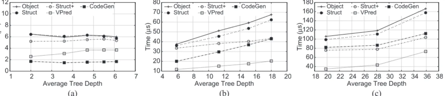
Fig. 4. Per-instance prediction times (in microseconds), averaged across cross-validation folds (100 ensembles per fold for LETOR and MSLR, and 20 ensembles for C14) using LambdaMART on different datasets. (a) LETOR-MQ2007. (b) MSLR-WEB10K. (c) C14.
We used the range of values suggested by Ganjisaffar
et al. [2] for maximum number of leaves. For each condi-tion, we report the average depth of the trees that were actually learned, along with the number of trees in the ensemble (i.e., number of boosting stages). Statistical sig-nificance was determined using the Wilcoxon test (p-value 0.05); none of the differences on the LETOR dataset were significant.
Results show that on LETOR, tree depth makes no signif-icant difference, whereas deeper trees yield better quality results on MSLR and C14. However, there appears to be little difference between 50 and 70 max leaves on MSLR. These results make sense: to exploit larger feature spaces we need deeper trees.
Turning to performance results, Fig.4 illustrates per-instance prediction speed for various implementations on the learning-to-rank datasets. Note that this is on the entire
TABLE 3
Average NDCG Values, Average Number of Trees, and Average Tree Depth (95% Confidence Intervals in Parentheses) Measured Across the Folds Using Various
Settings for Max Number of Leaves (L)
For MSLR, + and ∗ show statistically significant improvements over models obtained by setting max leaves to 10 and 30 respectively. For C14,+and∗show improvements over 70 and 110 respectively.
ensemble, with latencies now measured in microseconds instead of nanoseconds. As described above, the trees were trained with different settings of max leaves; the x-axis plots the tree depths from Table3. In this set of experiments, we used the VPREDapproach with the vectorization parameter set to 8 for LETOR and 16 for MSLR and C14.
The results from the synthetic datasets mostly carry over to these learning-to-rank datasets. OBJECT is the slowest implementation and STRUCT is slightly faster. On the LETOR dataset, STRUCT is only slightly slower than STRUCT+, but on MSLR and C14, STRUCT+ is much faster than STRUCTin most cases. While on LETOR it is clear that there is a large performance gap between CODEGEN and the other approaches, the relative advantages of CODEGEN
decrease with deeper trees and larger feature vectors (which is consistent with the synthetic results). VPREDoutperforms all other techniques, including CODEGEN on MSLR and
C14 but is slower than CODEGEN on LETOR. Since many in the community consider the LETOR dataset to be out of date with an impoverished feature set, more credence should be given to the MSLR and C14 results.
To conclude: for end-to-end tree-based ensembles on real-world learning-to-rank datasets, we can achieve both speed and flexibility. With a combination of predication and vectorization, we can make predictions faster than using statically-generated if-else blocks, yet retain the flexibility in being able to specify the model dynamically, which enables rapid experimentation.
6
D
ISCUSSION ANDF
UTUREW
ORKOur experiments show that predication and vectorization are effective techniques for substantially increasing the per-formance of tree-based models, but one potential objection might be: are we measuring the right thing? In our experi-ments, prediction time is measured from when the feature vector is presented to the model to when the prediction is made. Critically, we assume that features have already been computed. What about an alternative architecture where features are computed lazily, i.e., when the predicate at a tree node needs to access a particular feature?
This alternative architecture where features are com-puted on demand is very difficult to study, since results would be highly dependent on the implementa-tion of the feature extracimplementa-tion algorithm—which in turn depends on the underlying data structures (e.g., layout of the inverted indexes), compression techniques, how computation-intensive the features are, etc. However, there
TABLE 4
Average Percentage of Examined Features (Variance in Parentheses) Across Cross-Validation Folds Using
Various Max Leaves Settings
is a much easier way to study this issue—we can trace the execution of the full tree ensemble and keep track of the fraction of features that are accessed. If during the course of making a prediction, most of the features are accessed, then there is little waste in computing all the features first and then presenting the complete feature vector to the model.
Table 4shows the average fraction of features accessed in the final ensembles for all three learning-to-rank datasets, with different max leaves configurations. It is clear that for all datasets most of the features are accessed during the course of making a prediction, and in the case of the MSLR and C14 datasets, nearly all the features are accessed all the time (especially with deeper trees, which yield higher effectiveness). Therefore, it makes sense to sep-arate feature extraction from prediction. In fact, there are independently compelling reasons to do so: a dedicated feature extraction stage can benefit from better reference locality (when it comes to document vectors, postings, or whatever underlying data structures are necessary for com-puting features). Interleaving feature extraction with tree traversal may lead to “cache churn”, when a particular data structure is repeatedly loaded and then displaced by other data.
Returning to the point brought up in the introduction, another natural question is: do these differences actually matter, in the broader context of real-world search engines? This is of course a difficult question to answer and highly dependent on the actual search architecture, which is a com-plex distributed system spanning hundreds of machines or more. Here, however, we venture some rough estimates. From Fig.4(c), on the C14 dataset, we see that compared to CODEGEN, VPREDreduces per-instance prediction time from around 110μs to around 70μs (for max leaves
set-ting of 150); this translates into a 36% reduction in latency per instance. In a web search engine, the learning to rank algorithm is applied to a candidate list of documents that is usually generated by other means (e.g., scoring with BM25 and a static prior). The exact details are propri-etary, but the published literature does provide some clues. For example, Cambazoglu et al. [34] (authors from Yahoo!) experimented with reranking 200 candidate documents to
produce the final ranked list of 20 results (the first two pages of search results). From these numbers, we can com-pute the per-query reranking time to be 22ms using the CODEGEN approach and 14ms with VPRED. This trans-lates into an increase from 45 queries per second to 71 queries per second on a single thread for this phase of the search pipeline. Alternatively, gains from faster prediction can be leveraged to rerank more results or compute more features—however, how to best take advantage of addi-tional processor cycles is beyond the scope of this work. This simple estimate suggests that our optimizations can make a noticeable difference in web search, and given that our techniques are relatively simple—the predication and vectorization optimizations seem worthwhile to implement. Thus far, all of our experiments have been performed on a single thread, despite the fact that multi-core processors are ubiquitous today. We leave careful consideration of this issue for future work, but present some preliminary results here. There are two primary ways we can take advantage of multi-threaded execution: the first is to reduce latency by exploiting intra-query parallelism, while the second is to increase throughput by exploiting inter-query parallelism. We consider each in turn.
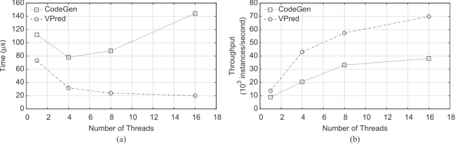
Since each tree model is comprised of an ensemble of trees, parallelism at an ensemble level can be obtained by assigning each thread to work on a subset of trees. This has the effect of reducing prediction latency. Fig. 5(a) shows the impact of this approach on prediction time using the C14 dataset with max leaves set to 150. By using 16 threads, latency decreases by 70% compared with a single-threaded implementation for VPRED. Note that since our machine has only eight physical cores, the extra boost obtained in going from 8 to 16 threads comes from hyper-threading. The small performance difference between the two differ-ent conditions suggests that our VPRED implementation
is effectively utilizing available processor resources (hence, the gains obtained from hyper-threading are limited). For CODEGEN, we observe a 30% improvement in latency by going from 1 to 4 threads. However, adding more threads actually increases prediction time.
The alternative multi-threaded design is to use each thread to independently evaluate instances using the entire ensemble. This exploits inter-query parallelism and increases throughput. More precisely, each thread evaluates one test instance using CODEGEN or v test instances (the batch size) in the case of VPRED. Fig. 5(b) shows the gain in throughput (number of test instances per second) for different number of threads on the C14 dataset with max leaves set to 150. Comparing implementations with a single thread and 16 threads, throughput increases by 320% (from 9K to 38K instances/second) for CODEGENand 400% (from 14K to 70K instances/second) for VPRED. This shows that
VPREDbenefits more from multi-core processors.
We note that these represent preliminary experiments on straightforward extensions of our optimizations to multi-threaded implementations. As part of future work, we will further explore how multi-core architectures impact the techniques discussed in this paper.
During the course of our experiments, we noticed that one assumption of our implementations did not appear to be fully valid: we assumed that all paths are equally likely
(a) (b)
Fig. 5. Impact of number of threads on latency and throughput, using C14 with max leaves of 150. (a) Each thread evaluates instances using a subset of trees in the ensemble, thus exploiting intra-query parallelism to reduce latency. (b) Each thread operates independently on instances, thus exploiting inter-query parallelism to increase throughput.
in a tree, i.e., that at each node, the left and right branches are taken with roughly-equal frequency. However, this is often not the case in reality, as the feature thresholds fre-quently divide the feature space unevenly. To the extent that one branch is favored over another, branch prediction pro-vides non-predicated implementations (i.e., if-else blocks) an advantage, since branch prediction will guess correctly more often, thus avoiding processor pipeline stalls.
One promising future direction to address the above issue is to adapt the model learning process to prefer bal-anced trees and predicates that divide up the feature space evenly. We believe this can be incorporated into the learn-ing algorithm as a penalty on certain tree topologies, much in the same way that regularization is performed on the objective in standard machine learning. Thus, it is perhaps possible to jointly learn models that are both fast and good, as in the “learning to efficiently rank” framework [31]–[33] (see discussion in Section2.2). Some preliminary results are reported in Asadi and Lin [36] with the CODEGEN
implementation of trees, but there is much more to be done. Finally, for specific tasks such as top k retrieval in learning to rank, we believe that there are many optimiza-tion opportunities that take advantage of the fact that we need to evaluate multiple test instances in order to gen-erate a document ranking. Our current approach assumes document-at-a-time evaluation, where the entire tree-based ensemble is applied to a single test instance before mov-ing to the next. Another possibility, and perhaps more promising, is tree-at-a-time evaluation, where we inter-leave operations on multiple test instances. Cambazoglu
et al. [34] considered both approaches in their early exits, but we believe that their techniques need to be revisited in the context of our work and from the perspective of architectural-conscious optimizations.
7
C
ONCLUSIONModern processor architectures are incredibly complex because technological improvements have been uneven. This paper examined three different issues: optimizing memory layout for cache locality, eliminating the cost of branch mispredicts, and masking memory latencies.
Although there are well-known techniques for tackling these challenges, researchers must be aware of them and explicitly apply them. The database community has been exploring these issues for quite some time now, and in this respect the information retrieval, machine learning, and data mining communities are behind.
In this paper, we demonstrate that two relatively simple techniques, predication and vectorization, coupled with a more compact memory layout, can significantly accelerate the runtime performance for tree-based models, both on synthetic data and on real-world learning-to-rank datasets. Our work enriches the literature on architecture-conscious optimizations for machine learning algorithms and presents a number of future directions worth pursuing.
8
A
CKNOWLEDGMENTSThis work was supported in part by the U.S. NSF under awards IIS-0916043, IIS-1144034, and IIS-1218043, and in part by the Dutch National Program COMMIT. Any opin-ions, findings, or conclusions are the authors’ and do not necessarily reflect those of the sponsors. The authors would like to thank the anonymous reviewers for their helpful suggestions in improving this work. N. Asadi’s deepest gratitude goes to Katherine, for her invaluable encourage-ment and wholehearted support. J. Lin is grateful to Esther and Kiri for their loving support and dedicates this work to Joshua and Jacob.
R
EFERENCES[1] C. J. C. Burges, “From ranknet to lambdarank to lambdamart: An overview,” Microsoft Res., Redmond, WA, USA, Tech. Rep. MSR-TR-2010-82, 2010.
[2] Y. Ganjisaffar, R. Caruana, and C. V. Lopes, “Bagging gradient-boosted trees for high precision, low variance ranking models,” in Proc. 34th SIGIR, Beijing, China, 2011, pp. 85–94.
[3] S. Tyree, K. Q. Weinberger, and K. Agrawal, “Parallel boosted regression trees for web search ranking,” in Proc. 20th Int. Conf.
WWW, Hyderabad, India, 2011, pp. 387–396.
[4] H. Li, Learning to Rank for Information Retrieval and Natural
Language Processing. San Rafael, CA, USA: Morgan & Claypool,
2011.
[5] B. Panda, J. S. Herbach, S. Basu, and R. J. Bayardo, “PLANET: Massively parallel learning of tree ensembles with mapreduce,” in Proc. 35th Int. Conf. VLDB, Lyon, France, 2009, pp. 1426–1437.
[6] G. Ge and G. W. Wong, “Classification of premalignant pancreatic cancer mass-spectrometry data using decision tree ensembles,”
BMC Bioinform., vol. 9, Article 275, Jun. 2008.
[7] L. Schietgat et al., “Predicting gene function using hierarchical multi-label decision tree ensembles,” BMC Bioinform., vol. 11, Article 2, Jan. 2010.
[8] A. Criminisi, J. Shotton, and E. Konukoglu, “Decision forests: A unified framework for classification, regression, density estimation, manifold learning and semi-supervised learn-ing,” Found. Trends Comput. Graph. Vis., vol. 7, no. 2–3, pp. 81–227, 2011.
[9] N. Johnson et al., “Financial black swans driven by ultrafast machine ecology,” arXiv:1202.1448v1, 2012.
[10] A. Ailamaki, D. J. DeWitt, M. D. Hill, and D. A. Wood, “DBMSs on a modern processor: Where does time go?” in Proc. 25th Int.
Conf. VLDB , Edinburgh, U.K., 1999, pp. 266–277.
[11] J. Rao and K. A. Ross, “Cache conscious indexing for decision-support in main memory,” in Proc. 25th Int. Conf. VLDB, Edinburgh, U.K., 1999, pp. 78–89.
[12] K. A. Ross, J. Cieslewicz, J. Rao, and J. Zhou, “Architecture sensi-tive database design: Examples from the columbia group,” IEEE
Data Eng. Bull., vol. 28, no. 2, pp. 5–10, Jun. 2005.
[13] M. Zukowski, P. Boncz, N. Nes, and S. Héman, “MonetDB/X100—A DBMS in the CPU cache,” IEEE Data
Eng. Bull., vol. 28, no. 2, pp. 17–22, Jun. 2005.
[14] P. A. Boncz, M. L. Kersten, and S. Manegold, “Breaking the mem-ory wall in MonetDB,” Commun. ACM, vol. 51, no. 12, pp. 77–85, 2008.
[15] K. Olukotun and L. Hammond, “The future of microprocessors,”
ACM Queue, vol. 3, no. 7, pp. 27–34, 2005.
[16] B. Jacob, The Memory System: You Can’t Avoid It, You Can’t Ignore
It, You Can’t Fake It. San Rafael, CA, USA: Morgan & Claypool,
2009.
[17] D. I. August, W. W. Hwu, and S. A. Mahlke, “A framework for balancing control flow and predication,” in Proc. 30th MICRO, North Carolina, NC, USA, 1997, pp. 92–103.
[18] H. Kim, O. Mutlu, Y. N. Patt, and J. Stark, “Wish branches: Enabling adaptive and aggressive predicated execution,” IEEE
Micro, vol. 26, no. 1, pp. 48–58, Jan./Feb. 2006.
[19] P. A. Boncz, M. Zukowski, and N. Nes, “MonetDB/X100: Hyper-pipelining query execution,” in Proc. 2nd Biennial CIDR, Pacific Grove, CA, USA, 2005.
[20] K. M. Svore and C. J. C. Burges, “Large-scale learning to rank using boosted decision trees,” in Scaling Up Machine Learning. Cambridge, U.K.: Cambridge Univ. Press, 2011.
[21] C. Ulmer, M. Gokhale, B. Gallagher, P. Top, and T. Eliassi-Rad, “Massively parallel acceleration of a document-similarity classi-fier to detect web attacks,” J. Parallel Distrib. Comput., vol. 71, no. 2, pp. 225–235, 2011.
[22] T. Sharp, “Implementing decision trees and forests on a GPU,” in
Proc. 10th ECCV, Marseille, France, 2008, pp. 595–608.
[23] B. V. Essen, C. Macaraeg, M. Gokhale, and R. Prenger, “Accelerating a random forest classifier: Multi-core, GP-GPU, or FPGA?” in Proc. IEEE 20th Annu. Int. Symp. FCCM, Toronto, ON, Canada, 2012, pp. 232–239.
[24] K. Järvelin and J. Kekäläinen, “Cumulative gain-based evalua-tion of IR techniques,” ACM Trans. Inform. Syst., vol. 20, no. 4, pp. 422–446, 2002.
[25] J. Ye, J.-H. Chow, J. Chen, and Z. Zheng, “Stochastic gradient boosted distributed decision trees,” in Proc. 18th Int. CIKM , Hong Kong, China, 2009, pp. 2061–2064.
[26] C. Burges, R. Ragno, and Q. Le, “Learning to rank with nons-mooth cost functions,” in Proc. Adv. NIPS, Vancouver, BC, Canada, 2006, pp. 193–200.
[27] J. Friedman, “Greedy function approximation: A gradient boost-ing machine,” Ann. Statist., vol. 29, no. 5, pp. 1189–1232, 2001. [28] L. Breiman, J. Friedman, C. Stone, and R. Olshen, New York, NY,
USA: Classification and Regression Trees. Chapman and Hall, 1984. [29] L. Breiman, “Bagging predictors,” Mach. Learn., vol. 24, no. 2,
pp. 123–140, 1996.
[30] L. Breiman, “Random forests,” Mach. Learn., vol. 45, no. 1, pp. 5–32, 2001.
[31] O. Chapelle, Y. Chang, and T.-Y. Liu, “Future directions in learning to rank,” in Proc. JMLR: Workshop Conf., 2011, pp. 91–100. [32] L. Wang, J. Lin, and D. Metzler, “A cascade ranking model for effi-cient ranked retrieval,” in Proc. 34th SIGIR, Beijing, China, 2011, pp. 105–114.
[33] Z. E. Xu, K. Q. Weinberger, and O. Chapelle, “The greedy miser: Learning under test-time budgets,” in Proc. 29th ICML, Edinburgh, U.K., 2012.
[34] B. B. Cambazoglu et al., “Early exit optimizations for additive machine learned ranking systems,” in Proc. 3rd ACM Int. Conf.
WSDM, New York, NY, USA, 2010, pp. 411–420.
[35] O. Chapelle and Y. Chang, “Yahoo! learning to rank challenge overview,” J. Mach. Learn. Res. – Proc. Track, vol. 14, pp. 1–24, Jun. 2010.
[36] N. Asadi and J. Lin, “Training efficient tree-based models for document ranking,” in Proc. 34th ECIR , Moscow, Russia, 2013.
Nima Asadi is a Ph.D. candidate in computer science at the University of Maryland, College Park, MD, USA. His current research interests include scalability and efficiency in information retrieval, learning to rank, and large-scale data processing.
Jimmy Lin is an Associate Professor at the iSchool, University of Maryland, College Park, MD, USA, affiliated with the Department of Computer Science and the Institute for Advanced Computer Studies. His current research interests include intersection of information retrieval and natural language processing, with a focus on massively distributed data analytics in cluster-based environments.
Arjen P. de Vries is a Tenured Researcher at Centrum Wiskunde and Informatica (CWI), leading the Information Access Research Group, and is a Full Professor (0.2 fte) in the area of Multimedia Data Management at the Technical University of Delft, Delft, Netherlands. He studies the intersection of information retrieval and databases. He has held General and Programme Chair positions at SIGIR 2007, CIKM 2011, and ECIR 2012 and 2014. He is a member of the TREC PC and a steering committee member of the Initiative for the Evaluation of XML Retrieval (INEX). In November 2009, he co-founded Spinque: a CWI spin-off that provides integrated access to any type of data, customized for informa-tion specialist or end user, to produce effective and transparent search results.
For more information on this or any other computing topic, please visit our Digital Library at www.computer.org/publications/dlib.