Small Sample Properties of Forecasts from
Autoregressive Models under Structural Breaks
∗
M. Hashem Pesaran
University of Cambridge and USCAllan Timmermann
University of California, San DiegoMay 2003, this version February 2004
Abstract
This paper develops a theoretical framework for the analysis of small-sample properties of forecasts from general autoregressive models under structural breaks. Finite-sample results for the mean squared forecast er-ror of one-step ahead forecasts are derived, both conditionally and uncon-ditionally, and numerical results for different types of break specifications are presented. It is established that forecast errors are unconditionally unbi-ased even in the presence of breaks in the autoregressive coefficients and/or error variances so long as the unconditional mean of the process remains un-changed. Insights from the theoretical analysis are demonstrated in Monte Carlo simulations and on a range of macroeconomic time series from G7 countries. The results are used to draw practical recommendations for the choice of estimation window when forecasting from autoregressive models subject to breaks.
JEL Classifications: C22, C53.
Key Words: Small sample properties of forecasts, MSFE, structural breaks, autoregression, rolling window estimator.
∗We are grateful to the editor, four referees, and seminar participants at Cass Business
School (London) for helpful comments on an earlier version of the paper. We would also like to thank Mutita Akusuwan for excellent research assistance.
1. Introduction
Autoregressive models are used extensively in forecasting throughout economics and finance and have proved so successful and difficult to outperform in practice that they are frequently used as benchmarks in forecast competitions. Due in large part to their relatively parsimonious form, autoregressive models are frequently found to produce smaller forecast errors than those associated with models that allow for more complicated nonlinear dynamics or additional predictor variables, c.f. Stock and Watson (1999) and Giacomini (2002).
Despite their empirical success, there is now mounting evidence that the pa-rameters of autoregressive (AR) models fitted to many economic time series are unstable and subject to structural breaks. For example, Stock and Watson (1996) undertake a systematic study of a wide variety of economic time series and find that the majority of these are subject to structural breaks. Alogoskoufis and Smith (1991) and Garcia and Perron (1996) are other examples of studies that document instability related to the autoregressive terms in forecasting models. Clements and Hendry (1998) view structural instability as a key determinant of forecasting performance.
This suggests a need to study the behaviour of the parameter estimates of AR models as well as their forecasting performance when these models undergo breaks. Despite the interest in econometric models subject to structural breaks, little is known about the small sample properties of AR models that undergo discrete changes. In view of the widespread use of AR models in forecasting, this is clearly an important area to investigate. The presence of breaks makes the focus on small sample properties more relevant: even if the combined pre- and post-break sample is very large, the occurrence of a structural break means that the post-break sample will often be quite small so that asymptotic approximations may not be nearly as accurate as is normally the case.
A key question that arises in the presence of breaks is how much data to use to estimate the parameters of the forecasting model that minimizes a loss function such as root mean squared forecast error (RMSFE). We show that the RMSFE-minimizing estimation window crucially depends on the size of the break as well as its direction (i.e., does the break lead to higher or lower persistence) and which parameters it affects (i.e., the mean, variance or autoregressive slope parameters). In some situations the optimal estimation window trades off an increased bias
introduced by using pre-break data against a reduction in forecast error variance resulting from using a longer window of the data. However, in other situations the small sample bias in the autoregressive coefficients may in fact be reduced after introducing pre-break data if the size of the break is small or even when the break is large provided that it is in the right direction (e.g., when persistence declines).
In the presence of parameter instability it is common to use a rolling window estimator that makes use of afixed number of the most recent data points, although the size of the rolling window is based on pragmatic considerations rather than an empirical analysis of the underlying time series process. Another possibility would be to test for breaks in the parameters and/or error variances and only use data after the most recent break, assuming a break is in fact detected. Alternatively, if no statistically significant break is found, an expanding window estimator could be used. Our theoretical analysis allows us to better understand when each of these procedures is likely to work well and why it is generally best to use pre-break data when forecasting using autoregressive models. First, breaks in the autoregressive parameters need not introduce bias in the forecasts (at least unconditionally). This tends to happen when an autoregressive coefficient declines after a break or the break only occurs in the intercept or variance parameter. Including pre-break data in such cases will tend to lead to a decline in RMSFE due to both a smaller squared bias and a reduction in the variance of the parameter estimate. Furthermore, in practice, there is likely to be a considerable error in detecting and estimating the point of the break of the autoregressive model. This leads to a worse performance of a post-break estimation procedure but also makes determination of the length of a rolling window more difficult.
Several practical recommendations emerge from our analysis regarding the choice of estimation window when forecasting from autoregressive models. First, for the macroeconomic data examined here, in general it appears to be difficult in prac-tice to outperform expanding or long rolling window estimation methods. Unlike the case with exogenous regressors, forecasts from autoregressive models can be seriously biased even if only post-break observations are used. Including pre-break data in estimation of autoregressive models can simultaneously reduce the bias and the variance of the forecast errors. In most applications where breaks are not too large, expanding window methods or rolling window procedures with relatively large window sizes are likely to perform well. This conclusion may not of course
carry over to longer data sets, e.g. high frequency financial data with thousands of observations, where estimation uncertainty can be reduced more effectively than with the relatively short macroeconomic data considered here.
The main contributions of this paper are as follows. First, we present a new procedure for computing the exact small sample properties of the parameters of AR models of arbitrary order, thus extending the existing literature that has focused on the AR(1) model. Our approach allows forfixed or random starting points and considers stationary AR models as well as models with unit root dynamics. We allow for the possibility of the AR model to switch from a unit root process to a stationary one andvice versa. Such regime switches could be particularly relevant to the analysis of inflation in a number of OECD countries since the first oil price shock in early 1970’s. In addition to considering properties such as bias in the para-meters, we also consider the RMSFE infinite samples. Second, we extend existing results on exact small sample properties of AR models to allow for a break in the un-derlying data generating process. We establish that one-step ahead forecast errors from AR models are unconditionally unbiased even in the presence of breaks in the autoregressive coefficients and in the error variances so long as the unconditional mean of the process remains unchanged. Our results also apply to models with unit roots. This extends Fuller (1996)’s result obtained for AR models with fixed parameters, and generalizes a related finding due to Clements and Hendry (1999, pp.39-42). Third, we present extensive numerical results quantifying the effect of the sizes of the pre-break and post-break data windows on parameter bias and RMSFE. Fourth, we undertake an empirical analysis for a range of macroeconomic time series from the G7 countries that compares the forecasting performance of expanding window, rolling window and post-break estimators. This analysis which allows for multiple breaks at unknown times confirms that, at least for macroeco-nomic time series such as those considered here, it is generally best to use pre-break data in estimation of the forecasting model.
The outline of the paper is as follows. Section 2 provides a brief overview of the small sample properties of the first-order autoregressive model that has been extensively studied in the extant literature. Theoretical results allowing us to characterize the small sample distribution of the parameters and forecast errors of autoregressive models are introduced in Section 3. Section 4 presents numerical results for AR models subject to breaks and Section 5 presents empirical results
for a range of macroeconomic time series. Section 6 concludes with a summary and a discussion of possible extensions to our work.
2. Small Sample Properties of Forecasts from Autoregressive Models A large literature has studied small sample properties of estimates of the parameters of autoregressive models. The majority of studies has concentrated on deriving either exact or approximate small sample results for the distribution of ˆαT and
ˆ
βT, the Ordinary Least Squares (OLS) estimators of α and β, in the first-order autoregressive (AR(1)) model
yt=α+βyt−1+σεt, t= 1,2, ..., T, εt∼iid(0,1). (1)
Analysis of the small sample bias of ˆβT dates back to at least Bartlett (1946). Early studies focus on the stationary AR(1) model without an intercept (α = 0,
|β| < 1) but have been extended to higher order models with intercepts (Sawa (1978)) and exogenous regressors (Grubb and Symons (1987), Kiviet and Phillips (1993, 2003a)). Assuming stationarity (|β| < 1), ˆβT has been shown to have an asymptotic normal distribution and its finite-sample distribution has been studied by Phillips (1977) and Evans and Savin (1981). The case with a unit root, β = 1, has been studied by, inter alia, Banerjee, Dolado, Hendry and Smith (1986), Phillips (1987), Stock (1987), Abadir (1993) and Kiviet and Phillips (2003b).
To a forecaster, the bias in ˆαT and ˆβT is of direct interest only to the extent
that it might adversely influence the forecasting performance. Ullah (2003) pro-vides an extensive discussion and survey of the properties of forecasts from the AR(1) model. Box and Jenkins (1970) characterized the asymptotic mean squared forecast error (MSFE) for a stationaryfirst-order autoregressive process considering both the single-period and multi-period horizon. Assuming a stationary process, Copas (1966) used Monte Carlo methods to study the MSFE of least-squares and maximum likelihood estimators under Gaussian innovations.
In practice, the conditional forecast error is of more interest than the uncon-ditional error since the data needed to compute conuncon-ditional forecasts is always available. A comprehensive asymptotic analysis for the stationary AR(p) model is provided in Fuller and Hasza (1981) and Fuller (1996). Using Theorem 8.5.3 in
Fuller (1996) it is easily seen that, conditional onyT, M SF E(ˆyT+1|yT) = E £ (yT+1−yTˆ +1)2|yT ¤ = σ2(1 + 1 T) + 1−β2 T µ yT − α 1−β ¶2 +O(T−3/2).
This yields the more familiar unconditional result
M SF E(ˆyT+1) =E(yT+1−yTˆ +1)2 =σ2(1 +
2
T) +O(T
−3/2).
Generalizations to AR(p) and multi-step forecasts are also provided in Fuller (1996, pp. 443-449), where it is established that the forecast error,yT+1−yTˆ +1,is unbiased
in small samples assuming εt has a symmetric distribution and E(|yTˆ +1|) < ∞.
This is particularly noteworthy considering the often large small sample bias asso-ciated with estimates of the autoregressive parameters.
3. AR(p) Model in the Presence of Structural Breaks
In parallel with the work on the small sample properties of estimates of autoregres-sive models, important progress has been made in testing for and estimating both the time and the size of breakpoints, as witnessed by the recent work of Andrews (1993), Andrews and Ploberger (1996), Bai and Perron (1998, 2003), Banerjee, Lumsdaine and Stock (1992), Chu, Stinchcombe and White (1996), Chong (2001), Elliott and Muller (2002), Hansen (1992), Inclan and Tiao (1994) and Ploberger, Kramer and Kontrus (1989).
Building on this work we consider the small sample problem of estimation and forecasting with AR(p) models in the presence of structural breaks. For this pur-pose, we consider the following AR(p) model defined over the periodt= 1,2, ..., T; and assumed to have been subject to a single structural break at time T1 :
yt=
(
α1+β11yt−1 +β12yt−2+...+β1pyt−p+σ1εt, , for t≤T1, α2+β21yt−1 +β22yt−2+...+β2pyt−p+σ2εt, , for t > T1,
. (2) As before εt ∼ iid(0,1) for all t. For the analysis of the unit root case it is also
convenient to consider the following parameterization of the intercept terms,αi:
where β∗i =
Pp
j=1βij,=τp0βi, βi = (βi1,βi2, ...,βip)0 and τp is a p×1 unit vector.
Note that −(1−β∗i) also represents the coefficient of yt−1 in the error correction
representation of (2).
This specification is quite general and allows for intercept and slope shifts, as well as a change in error variances immediately aftert =T1. It is also possible for
the yt process to contain a unit root (or be integrated of order 1) in one or both of the regimes. The integration property of yt under the two regimes is governed by whether β∗i = 1 or β∗i <1. More specifically, we shall assume that the roots of
p
X
j=1
λjβij−1 = 0, for i= 1,2, (4)
lie on or outside the unit circle.1 As µ
i is allowed to vary freely, the intercepts
αi =µi(1−β∗i) are unrestricted when the underlying AR processes are stationary.
However, to avoid the possibility of generating linear trends in the yt process, the intercepts are restricted (αi = 0) in the presence of unit roots. In the stationary
case µi represents the unconditional mean of yt in regimei. In the unit root case µi is not identified and we haveE(∆yt) = 0.
Analysis of forecast errors from AR models subject to structural change have been recently addressed by Clements and Hendry (1998,1999). However, these authors either abstract from the problem of parameter uncertainty, or only allow for it assuming that the parameters of the AR model remain unchanged during the estimation period. Consider first the analysis provided in Clements and Hendry (1998, pp.168-171), where it is assumed that parameters are known and the break takes place immediately prior to the forecasting period. In this case the one-step ahead forecast error is given by
yT+1−yT˜ +1 =µ2(1−β∗2)−µ1(1−β∗1) +x0T (β2−β1) +σ2εT+1,
wherexT = (yT, yT−1, ..., yT−p+1)0, (µ1,β1) are the parameters prior to the forecast
period, and (µ2,β2) are the parameters during the forecast period, here T + 1.
Following Clement and Hendry and noting thatβ∗i =τ0pβi, it is easily verified that
yT+1−yT˜ +1 = (µ2−µ1) (1−β∗2) + (β2−β1)0(xT −µ1τp) +σ2εT+1,
1Our analysis can also allow for the possibility of y
t being integrated of order two in one or
and
E(yT+1−yT˜ +1) = (µ2−µ1) (1−β∗2) + (β2−β1)0E(xT −µ1τp).
In the case where yt is stationary we haveE(xT −µ1τp) = 0, and E(yT+1−yT˜ +1) = (µ2−µ1) (1−β∗2),
which does not depend on the size of the break in the slope coefficients,β2−β1, and will be zero whenµ2 =µ1. This is an interesting theoretical result but its relevance is limited in practice where estimates of (µ1,β1) based on past observations need to be used. One of the contributions of this paper might be viewed as identifying the circumstances under which the above result is likely to hold in the presence of estimation uncertainty.
In a related contribution Clements and Hendry (1999, pp. 39-42) consider the effect of estimation uncertainty on the forecast error decomposition using a
first-order vector autoregressive model, and conclude estimation uncertainty to be relatively unimportant. However, their analysis assumes that the estimation is carried out immediately prior to the break, based on a correctly specified model which is not subject to any breaks. The assumption that parameters have been stable prior to forecasting is clearly restrictive, and it is therefore important that a more general framework is considered where the effect of estimation uncertainty can be analysed even in the presence of multiple breaks in the parameters (slope coefficients as well as error variances) over the estimation period. In this paper we provide such a framework in the case of AR(p) models subject to a single break point over the estimation period. But, it should become clear that the analysis readily extends to two or more break points.2
In particular, our interest in this paper lies in the point (or probability) fore-cast of yT+1 conditional on ΩT ={y1, y2, ..., yT} in the context of the break point
specification (2). In the case where the post-break window size, v2 = T −T1 is
sufficiently large (v2 → ∞), the structural break is relatively unimportant and the
forecast of yT+1 can be based exclusively on the post-break observations. However,
whenv2 is small it might be worthwhile to base the forecasting model on pre-break
2Explicitly allowing for breaks and parameter uncertainty prior to forecasting also raises the
issue of the choice of observation window discussed in related papers in Pesaran and Timmermann (2002, 2003).
as well as post-break observations. The number of pre-break observations, which we denote by v1, then becomes a choice parameter. In what follows we assume T1
is known but consider forecastingyT+1 using the past T −m+p+ 1 observations,
m−p being the starting point of the estimation window, yT(m−p) = (ym−p, ym−p+1, ..., yT1, yT1+1..., yT)
0, (5)
with the pobservations ym−p, ym−p+1, ..., ym−1 treated as given initial values.3 The
length of the pre-break window is then given by v1 =T1−m+ 1, and the number
of time periods used in estimation is thereforev =v1+v2 =T−m+ 1. To simplify
the notations we shall consider values of v1 ≥p, or m ≤T1−p−1.
The point forecast of yT+1 conditional on yT(m−p) is given by
ˆ yT+1(m) = ˆαT(m) +x0TβˆT(m), where xT = (yT, yT−1, ..., yT−p+1)0, βˆT(m) = ³ ˆ β1T(m),βˆ2T(m), ...,βˆpT(m) ´0 , τv is
a v×1 vector of ones,Mτ =Iν −τv(τ0vτv)−1τ0v, and
XT (m) = (yT−1(m−1),yT−2(m−2), ...,yT−p(m−p)), so that ˆ βT(m) = [X0T(m)MτXT(m)]−1X0T(m)MτyT(m), (6) ˆ αT(m) = τ0 vyT(m)−τ0vXT (m)βˆT(m) v , (7)
The one-step ahead forecast error is
eT+1(m) =yT+1−yTˆ +1(m) =σ2εT+1−ξT(m), (8) where ξT(m) = [ˆαT(m)−α2] +x0T ³ ˆ βT(m)−β2´. (9) β2 = (β21,β22, ...,β2p)0 and α2 = µ2 ¡ 1−τ0 pβ2 ¢
. We consider both the uncon-ditional and conuncon-ditional mean squared forecast error given by Eε
¡ e2 T+1(m) ¢ and Eε ¡ e2 T+1(m)|ΩT ¢
, respectively, where the expectations operator Eε(·) is defined with respect to the distribution of the innovations εt. To the see how the MSFE
3Throughout the paper we shall use the notationy
depends on the starting point of the estimation window, m, note that εT+1 and ξT(m) are independently distributed and
Eε ¡ e2T+1(m)|ΩT ¢ =σ22+Eε ¡ ξ2T(m)|ΩT ¢ . (10)
To carry out the necessary computations, an explicit expression forξT(m) in terms
of the ε0ts is required. This is complicated and depends on the state of the process
just before the first observation is used for estimation.
For a given choice of m > pand afinite sample size T, the joint distribution of ˆ
βT(m) and ˆαT(m) depends on the distribution of the initial values
ym−1(m−p)= (ym−p, ym−p+1, ..., ym−1)0. (11)
We distinguish between the two important cases where the pre-break process is stationary and when it contains a unit root.
3.0.1. Pre-Break Process is Stationary
In the case where the pre-break regime is stationary and has been in operation for sufficiently long time, the distribution of ym−1(m−p) does not depend on m and
is given by
ym−1(m−p)∼N(µ1τp,σ21Vp), (12)
where Vp is defined in terms of the pre-break parameters. For example, forp= 1, V1 = 1/(1−β211), and for p= 2 V2 = 1 (1 +β12)£(1−β12)2−β211¤ Ã 1−β12 β11 β11 1−β12 ! .
3.0.2. Pre-Break Process is I(1)
If the pre-break process contains a unit root, the covariance of ym−1(m−p) is no
longer given by σ2
1Vp and in general depends on m. Under a pre-break unit root,
β∗1 = 1 and the pre-break process is given by
∆yt=
p−1 X
j=1
δ1j∆yt−j+σ1εt, for t≤T1, (13)
whereδ1j =−Pp`=j+1β1`. The distribution of initial values can now be specified in
an assumption concerning the first observation in the sample, y1. In what follows
we assume that y1 is given by
y1 =µ1+ωε1, (14)
where ω will be treated as a free parameter, and ε1 ∼ N(0,1). Using (13) and (14) it is now possible to derive the distribution of the initial values, ym−1(m−p)
= (ym−p, ym−p+1, ..., ym−1)0, noting that
ym−i =y1+∆y2+...+∆ym−i, for i= 1,2, ..., p.
In the AR(1) case we have
∆yt=σ1εt, for t= 2,3, ..., T1,
and in conjunction with (14) we have
ym−1 = y1+∆y2+...+∆ym−1
= µ1+ωε1+σ1(ε2+ε3+...+εm−1),
and hence ym−1 ∼N (µ1,V1,m), where
V1,m =ω2+ (m−2)σ21. (15)
For the AR(2) specification we haveym−1(m−2) = (ym−2, ym−1)0 ∼N(µ1τ2,V2,m),
where V2,m is derived in Appendix A.
3.1. OLS Estimates
Using (12) and (2) for t=m, m+ 1, ..., T, in matrix notations we have
B yT(m−p) =d+D ε, (16) where D=σ1 ψp 0 0 0 Iν1 0 0 0 (σ2/σ1)Iν2 , d=µ1 τp (1−β∗1)τv1 (µ2/µ1) (1−β∗2)τv2 , (17) B= Ip 0 0 B21 B22 0 0 B32 B33 . (18)
The sub-matrices, Bij, depend only on the slope coefficients, β1 and β2 and are
defined in Appendix B.Iν1 andIν2 are identity matrices of orderν1 andν2,
respec-tively andε= (εm−p,εm−p+1, ...,εT)0 ∼N(0,Iν+p).
The form of ψp depends on whether the pre-break process is stationary or contains a unit root. Under the former ψp is a lower triangular Cholesky factor of Vp, namely Vp = ψpψ0p, where Vp is the covariance matrix of ym−1(m−p).
Appropriate expressions for Vp in the case of p= 1 and 2 are already provided in
Section 3.0.1. When the pre-break process has a unit root,ψp is given by the lower triangular Cholesky factor of Vp,m, which is given by (15) above for p = 1 and in
Appendix A by (38) for p= 2.
Using (40) derived in Appendix B, in general we have
yT−i(m−i) =Gi(c+Hε), for i= 0,1, ..., p, (19)
where Gi are v × (v + p) selection matrices defined by Gi = (0v×p−i...Iν...0v×i), H=B−1D, and c=B−1d. In particular, yT(m) =G0(c+Hε), and XT (m) = h G1(c+Hε),G2(c+Hε), ...,Gp(c+Hε) i .
Therefore, in general the (i, j) element of the product moment matrix,X0
T (m)MτXT (m),
is given by (c+Hε)0G0
iMτGj(c+Hε), for i, j = 1,2, ..., p, and the jth element
of X0
T (m)MτyT(m) is given by (c+Hε)0G0jMτG0(c+Hε), for j = 1,2, ..., p.
Hence, βˆT(m) = ³βˆ1T(m),βˆ2T(m), ...,βˆpT(m)
´0
, is a non-linear function of the quadratic forms (c+Hε)0G0
iMτGj(c+Hε), for i = 1,2, ...p, and j = 0,1, ..., p,
with known matrices H,Gi, c, and ε∼N(0,Iν+p). Similarly, using (7) we have
ˆ αT(m) =v−1τ0vG0(c+Hε)−v−1τ0v p X i=1 Gi(c+Hε)ˆβiT(m). (20)
In the AR(1) case these results simplify to ˆ βT(m) = (c+Hε)0G10MτG0(c+Hε) (c+Hε)0G0 1MτG1(c+Hε) , (21) and ˆ αT(m) =v−1τ0vG0(c+Hε)−v−1τ0vG1(c+Hε)ˆβT(m). (22)
Using the above results in (6) it is now easily seen that in generalβˆT(m) depends on the ratios, µ1/σ1,σ1/σ2 andµ1/µ2 (orµ2/µ1), whilst ˆαT(m) depends on all the
four coefficients, µ1, µ2, σ1, andσ2, individually. Two cases of special interest arise
when there is no mean shift in the model, and when the post-break process contains a unit root. In both cases, as shown in Appendix B,Gic=κτv whereκ=µwhen
there is no mean shift (i.e. µ1 =µ2 = µ), and κ =µ1 if there is a mean shift but
β∗2 = 1. Under either of these two special cases we have MτGic=0, for all i, and ˆ
βT(m) will be a function of the quadratic terms, ε0H0G0iMτGjHε, which depend
only on the ratio of the error variances, σ1/σ2. These results also establish the following proposition:
Proposition 1 Under µ1 = µ2 or if β∗1 < 1 and β∗2 = 1, βˆT(m) defined by (6)
does not depend on the scale of the error variances (σ2
1,σ22) or the unconditional means, µ1, µ2, and is an even function of ε.
This proposition plays a key role in the analysis of prediction errors below. It is also worth noting that βˆT(m) will continue to be an even function of the errors in the more general case where the slope coefficients and/or the error variances are subject to multiple breaks, so long as the mean of the process remains unchanged. This proposition does not, however, extend to the OLS estimate of the intercept, ˆ
αT(m). To see this, using (20) and noting that under µ1 = µ2, or if β∗2 = 1,
Gic=µ1τv we have ˆ αT(m) =µ1 ³ 1−βˆ∗T(m)´+ µ τ0 vG0Hε v ¶ − p X i=1 µ τ0 vGiHε v ¶ ˆ βiT(m), (23) where ˆβ∗T(m) = Pp
i=1βˆiT(m) =τ0pβˆT(m). It is clear that in this case ˆαT(m) is an
odd function ofε, and depends on σ1,σ2 and µ1 individually.
3.2. Forecast Error Decomposition
Using (20) and (9) in (8), and recalling that α2 = µ2 ¡
1−τ0pβ2¢, then after some algebra the forecast error, eT+1(m), can be decomposed as
eT+1(m) =σ2εT+1−X1T(m)−X2T(m)−X3T(m), (24) where X1T(m) = µ τ0vG0c v −µ2 ¶ − p X i=1 µ τ0vGic v −µ2 ¶ ˆ βiT(m), (25)
X2T(m) = τ0vG0Hε v − p X i=1 µ τ0vGiHε v ¶ ˆ βiT(m), (26) and X3T(m) = (xT −µ2τp)0 ³ ˆ βT(m)−β2´. (27) The first term in this decomposition refers to future uncertainty which is indepen-dently distributed of the other terms. The second term,X1T(m), is due to the mean
shift and disappears under µ1 = µ2 = µ. Recall that in this case v−1τ0vGic=µ,
for all i.4 The third term, X2T(m), captures the uncertainty associated with the
unconditional mean of the process and reduces to zero if µ1 = µ2 = 0. The last
term represents the slope uncertainty and depends on whether the analysis is car-ried out unconditionally, or conditionally on xT = (yT, yT−1, ..., yT−p+1)0, in which
case the extent of the bias will generally depend on the size of the gap xT −µ2τp.
3.3. Unconditional MSFE
To obtain the unconditional form ofeT+1(m), we first note thatxT can be written
asSpyT(m), where Sp = (0p×(v−p)...Jp), and Jp is the p×pmatrix
Jp = 0 0 · · · 1 0 0 · · · 1 0 .. . ... · · · ... ... 0 1 · · · 0 0 1 · · · 0 0 .
Therefore, using (19) we have
xT −µ2τp = (SpG0c−µ2τp) +SpG0Hε,
and X3T(m), defined by (27), decomposes further as X3T(m) = (SpG0c−µ2τp)0 ³ ˆ βT(m)−β2 ´ + (SpG0Hε)0 ³ ˆ βT(m)−β2 ´ . 4See the last section of Appendix B. Note also thatX
1T(m) does not disappear ifβ∗2=τ0pβ2= 1, so long as µ16=µ2. However, underβ∗2=1, it simplifies to
X1T(m) = (µ1−µ2)
³
However, underµ1 =µ2 =µthe first term of X3T(m) vanishes and we have5 eT+1(m) = σ2εT+1−X2T(m)− ³ ˆ βT(m)−β2 ´0 SpG0Hε. (28)
Also under µ1 =µ2 =µ, eT+1(m), and hence Eε
£
e2T+1(m) ¤
, do not depend on the unconditional mean of the autoregressive process.
The computation ofEε
£
e2T+1(m) ¤
can be carried out via stochastic simulations. We have ˆ ER£e2T+1(m)¤=σ22+ 1 R R X r=1 h X1(rT)(m) +X2(Tr)(m) +X3(rT)(m)i2,
where the terms XiT(r)(m), i = 1,2,3 can be computed using random draws from ε∼N(0,Iν+p), which we denote byε(r), r= 1,2, ..., R. In particular,
X1(rT)(m) = µ τ0vG0c v −µ2 ¶ − p X i=1 µ τ0vGic v −µ2 ¶ ˆ β(iTr)(m), (29) X2(rT)(m) = τ 0 vG0Hε(r) v − p X i=1 Ã τ0vGiHε(r) v ! ˆ β(iTr)(m), (30) X3(rT)(m) = (SpG0c−µ2τp)0 ³ ˆ β(Tr)(m)−β2´+³SpG0Hε(r) ´0³ ˆ β(Tr)(m)−β2´, (31) and ˆβ(iTr)(m) denotes the estimate of βi based on ε(r). Assuming E
ε
£
e2
T+1(m) ¤
exists, then due to the independence ofε(r) across r, and the fact thatX(r)
iT (m) are
also independently and identically distributed across r, we have (asR → ∞) ˆ ER£e2T+1(m) ¤ p →Eε £ e2T+1(m) ¤ .
The following proposition generalizes Theorem 8.5.2 in Fuller (1996, page 445) to the case where estimation has been based on an AR(p) model which has been subject to breaks in the slope coefficients and/or error variances.
Proposition 2: The one-step ahead forecast errors, eT+1(m), defined by (8)
from the AR(p) model, (2), subject to a break in the AR coefficients (β1 6=β2) or a break in the innovation variance (σ2
1 6=σ22) are unbiased provided that:
(i) The probability distribution of ε∗ = (ε0,εT+1)0 is symmetrically distributed
aroundE(ε∗) = 0, and its first and second order moments exist;
5Note that in this caseS
(ii) The first-order moments of the estimated slope coefficients, ˆβiT(m), exist,
namely E¯¯¯βˆiT(m)¯¯¯<∞,for i= 1,2, ..., p;
(iii) There is no break in the mean of the process, µ1 =µ2.
Proof: Underµ1 =µ2, using (26) and (28), the prediction error can be written as eT+1(m) = σ2εT+1− ³ ˆ βT(m)−β2´0SpG0Hε − " τ0 vG0Hε v − p X i=1 µ τ0 vGiHε v ¶ ˆ βiT(m) # .
It is clear that under assumption (i) the terms σ2εT+1, β02SpG0Hε, and τ0vG0Hε,
which are linear functions of ε∗, have mean zero and we have
Eε[eT+1(m)] =−Eε h ˆ β0T(m)SpG0Hε i + p X i=1 Eε ·µ τ0vGiHε v ¶ ˆ βiT(m) ¸ .
Also under µ1 =µ2 and by Proposition 1, βˆT(m), is an even function of ε. Hence, ˆ
β0T(m)SpG0Hε, and (τ0vGiHε) ˆβiT(m) fori= 1,2, ..., pare odd functions of ε, and
under assumptions (i) and (ii) their expectations exist and are equal to zero by the symmetry assumption. Therefore,
Eε[eT+1(m)] = 0.
In the case where µ1 6= µ2, ˆβjT(m) is not an even function of ε, the term X1T
defined by (25) does not vanish and the prediction error given by (24), is no longer an odd function of ε, so it will, in general, not have a zero mean. ¥
Remark: Conditions under which moments of ˆβiT(m) exists in the case of
AR(1) models with fixed coefficients have been investigated in the literature and readily extends to AR(1) models subject to breaks. For the AR(1) model under
µ1 =µ2 we have [see (21)] ˆ βT(m) = ε0H0G01MτG0Hε ε0H0G0 1MτG1Hε .
Assuming that ε is normally distributed and applying a Lemma due to Smith (1988) to (ε0H0G0
ˆ
βT(m) exists ifRank(H0G01MτG1H) =v−1 =T−m >2r.6 Hence, ˆβT(m) has a
first-order moment if T > m+ 2. To our knowledge no such conditions are known for higher order AR processes, even with fixed coefficients.
Proposition 2 has important implications for the trade-off that exists in the estimation bias of the slope and intercept coefficients in the AR models even in the presence of breaks so long as µ1 =µ2 =µ. To see this notice from (22) that
E[ˆαT(m)−α2] =−µ E
h
ˆ
β∗T(m)−β∗2i.
This provides an interesting relationship between the small sample bias of the estimator of the intercept term, E[ˆαT(m)−α2], and the small sample bias of the
long-run coefficient,Ehβˆ∗T(m)−β∗2i. The estimator of the intercept term, ˆαT(m),
is unbiased only if the sample mean is zero. But, in general there is a spill-over effect from the bias of the slope coefficient to that of the intercept term.
For the AR(1) model the results simplify further and we have
E[ˆαT(m)−α2] =−µ E h ˆ βT(m)−β2i. (32) Since EhβˆT(m)−β2 i
<0, it therefore follows that
E[ˆαT(m)−α2] > 0 if µ >0, E[ˆαT(m)−α2] ≤ 0 if µ≤0.
Once again these results hold irrespective of whether β1 =β2 or not.
3.4. Conditional MSFE
As before we have
eT+1(m) =σ2εT+1−X1T(m)−X2T(m)−X3T(m),
where XiT(m), i = 1,2,3, are defined by (25), (26), and (27). In computing the conditional MSFE, defined byEε
¡
e2
T+1(m)|ΩT
¢
, wefix xT and integrate with
respect to the distribution ofε. Recall thatβˆT(m) and ˆαT(m) as defined in (6) and
(7) are only functions of ε and are hence not constrained by the terminal value, 6Note thatHis full rank,rank(G
xT.7 To investigate the effect of parameter estimation uncertainty we therefore draw values of ε independently ofxT.
Once again the results simplify when µ1 = µ2 = µ. In this case X1T(m) =
0, X2T(m) is an odd function of ε, and assuming that the distribution of ε is
symmetric we have Eε[eT+1(m)|ΩT] =−(xT −µτp)0Eε ³ ˆ βT(m)−β2 ´ .
Suppose p = 1, so that it is easy to characterize when xT is above or below the
mean. Then Eε[eT+1(m)|ΩT] = −(yT −µ)Eε ³ ˆ βT(m)−β2´. (33) Since, Eε ³ ˆ βT(m)−β2´<0, Eε[eT+1(m)|ΩT] = ( >0 if yT > µ ≤0 if yT ≤µ , (34)
and the estimated model under-predicts if the last observation is above the uncon-ditional mean (yT > µ), while conversely it over-predicts if the last observation is below the unconditional mean (yT < µ). Therefore, conditional predictions tend to be biased towards the unconditional mean of the process.
As with the unconditional MSFE, the computation of the conditional MSFE can also be carried out by stochastic simulations. In general, for a given value of xT,and using draws from ε∼N(0,Iν+p) we have
ˆ ER¡e2T+1(m)|ΩT ¢ =σ22+ 1 R R X r=1 h X1(rT)(m) +X2(rT)(m) + ˜X3(rT)(m)i2, (35)
where X1(rT)(m) and X2(rT)(m) are given by (29) and (30), as before, with the third term, ˜X3(rT)(m), now defined by
˜
X3(rT)(m) = (xT −µ2τp)0
³
ˆ
β(Tr)(m)−β2´. (36) Once again as R → ∞, we would expect ˆER¡e2
T+1(m)|ΩT ¢ p → Eε ¡ e2 T+1(m)|ΩT ¢ . 7This is consistent with the approach taken in calculating asymptotic results, c.f. Fuller (1996).
If we literally condition on the full path ofy-values inΩT, then ˆβT(m) and ˆαT(m) are of course
4. Numerical Results
Our approach is quite general and allows us to study the small sample properties of AR models in some detail. The existing literature has focused on the AR(1) model without a break, where the key parameters affecting the properties of the OLS estimators, ˆαT(m) and ˆβT(m), are the sample size and the persistence parameter,
β1. In our setting there are many more parameters to consider. In the absence of a break there are now p autoregressive parameters plus the intercept, α, and the innovation variance, σ2. Under a single break, we need to consider both the
pre- and post-break parameters - i.e. the AR coefficients (β1,β2), the intercepts (α1,α2) and the innovation variances (σ2
1,σ22). Furthermore, how the total sample
divides into pre- and post-break periods (v1 and v2) is now crucial to the bias in
the post-break parameter estimates and to the bias and variance of the forecast error.
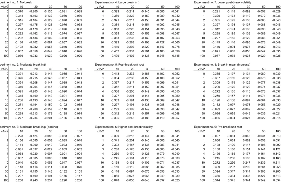
To ensure that our results are comparable to the existing literature, our bench-mark model is the AR(1) specification without a break (experiment 1 in Table 1). We study breaks in the autoregressive parameter in the form of both moderately sized (0.3) and large (0.6) breaks in either direction (experiments 2-4) as well as a unit root process in the post-break (experiment 5) or pre-break (experiment 9) period. We also consider pure breaks in the innovation variance (experiments 6 and 7), where σ changes between values of 1/4 and 1 or 4 and 1, and in the mean (experiment 8), where µchanges between 1 and 2. For convenience the parameter values assumed in each of the experiments are summarized in Table 1. Since our focus is on the effect of breaks on the bias and forecasting performance of AR models, results are presented as a function of the pre-break window size (v1) and
the post-break window size (v2).We vary v1 from zero (no pre-break information)
through 1, 2, 3, 4, 5, 10, 20, 30, 50 and 100, while the post-break window, v2, is
set at 10, 20, 30, 50 and 100.
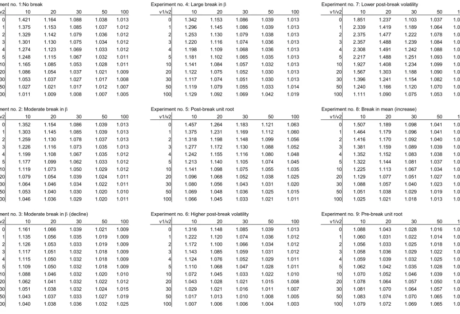
Simulation results are presented in Tables 2-5. Results are based on 50,000 Monte Carlo simulations with innovations drawn from an IID Gaussian distribu-tion.8 Table 2 shows the bias in ˆβ1 while Table 3 shows the conditional bias in the
forecast for a situation whereyT is above its mean, i.e.,yT =µ2+σ2.9 To measure
8We also considered an AR(2) specification to study the effect of higher order dynamics.
Results were very similar to those reported below and are available from the authors’ web site.
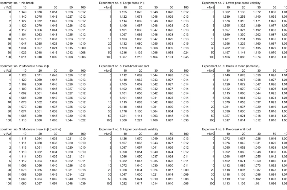
forecasting performance, Table 4 reports the unconditional RMSFE while Table 5 shows the RMSFE conditional on yT =µ2+σ2, as functions of the pre-break (v1)
and post-break (v2) window sizes. We condition on this particular value since if
yT =µ2 the conditional bias is zero while ifyT =µ2−σ2 the conditional bias takes the same value but with the sign reversed, c.f. (33).
4.1. Bias Results
First consider the bias in ˆβ1. In the absence of a break, ˆβ1 is downward biased with a bias that disappears as v1 and v2 increase and becomes quite small when
the combined sample v = v1 +v2 is sufficiently large.10 Notice the symmetry of
the results in v1 and v2 which follows since (under no break) only v1+v2 matters
for the bias.11 Once a break is introduced in the AR parameter, the bias in ˆβ1
continues to decline inv2 but need no longer decline monotonically as a function of
v1. The reason for this is simple: including pre-break data generated by a different
(less persistent) process introduces a new bias term in ˆβ1. It is only to the extent that this term is offset by a reduction in the small sample bias of the AR estimate that inclusion of pre-break data will lead to a bias reduction. Thus, whenv2 is very
large (e.g., 50 or 100 post-break observations) the small sample bias in ˆβ1 based
purely on post-break observations is already quite small. In this situation, inclusion of pre-break data will not lower the bias in ˆβ1. Conversely, when the post-break
sample is small (i.e.,v2 = 10−20 observations), the small sample bias in ˆβ1 is very
large and including up to 30 pre-break observations will actually reduce the bias under a moderately sized break. Naturally, if the break size is large (experiment 4), this effect is reduced since the true bias due to including pre-break observations in the estimation window dominates any reduction in the small sample bias in ˆβ1 true post-break values. To ensure comparability across the experiments they are based on the same random numbers.
10The bias estimates are in line with the well known Kendall (1954) approximation formula
E³βˆ1´−β1= −(1+ 3β1)
v +O(v
−3/2), v=v 1+v2. 11Recall from (32) that in the case of Gaussian errors the bias in ˆα
T(m) can be exactly inferred
from the bias of ˆβT(m) when there is no break in the mean. For this reason we focus our analysis on the bias in ˆβT(m).
based solely on post-break data for all but the smallest post-break window sizes. Interestingly, when the break is in the reverse direction (experiment 3) so that the true value of β1 declines, including a small number of pre-break data points
leads to a reduction in the bias in ˆβ1 even for very large post-break windows. For example, the bias in ˆβ1 is minimized by including 3 pre-break observations even
whenv2 = 100. The reason is again related to the direction of the small sample bias
in ˆβ1. Since ˆβ1 is downward biased, when the break is from high to low persistence, the (upward) bias introduced by inclusion of the more persistent pre-break data works in the opposite direction of the small sample (downward) bias in ˆβ1. For this reason the biases under a decline inβ1 tend to be smaller than the biases observed
when β1 increases at the time of the break.
Under a post-break unit root (experiment 5) the bias-minimizing pre-break window size is around 20 observations. Under a pre-break unit-root (experiment 9), bias is smallest for either v1 = 0 or v1 = 1. When a break occurs in the
innovation variance (experiments 6 and 7), the smallest bias is always achieved by the longest pre-break windows. The only difference to the case without a break is that the bias is no longer a symmetric function ofv1 andv2. Allowing for a break in
the mean (experiment 8), the forecast error is no longer unbiased unconditionally and the optimal pre-break window size rises to 100 irrespective of the value of v2.
Turning next to the conditional bias in the forecast, Table 3 shows that, in the absence of a break, the bias is positive when the prediction is made conditional on yT = µ2 +σ2, a value above the mean of the process. This is, of course, consistent with (34) and with the sign of the bias in ˆβ1. In general, the results for
the conditional bias in the forecast error mirror those of the bias in ˆβ1, except for the case with a break in the mean. Whereas the bias in ˆβ1 was reduced the larger
the value of v1 when the mean increases at the time of the break, the bias in the
forecast error is smallest when v1 = 0 and the mean increases assuming a large
post-break sample (v2 = 50 or 100).
4.2. Forecasting Performance
To measure forecasting performance for the AR(1) model, unconditional and con-ditional RMSFE values are shown in Tables 4 and 5. Under no break the uncon-ditional RMSFE is 1.15 for the smallest combined sample (v1 = 0, v2 = 10) and it
break in the AR coefficient, the unconditional RMSFE continues to decline as a function of v2 but it no longer declines monotonically inv1, the pre-break window.
Furthermore, the unconditional RMSFE no longer converges to one - its theoretical value in the absence of parameter estimation uncertainty - provided the ratiov1/v2
does not go to zero. For example, when v1 =v2 = 100, the unconditional RMSFE
under a moderate break inβ1is close to 1.02 as opposed to a value of 1.006 observed in the case without a break. This difference is due to the squared bias in the AR parameters introduced by including pre-break data points. Generally, the windows that minimize the unconditional RMSFE tend to be longer than the windows that minimize the bias. Increasing the window size beyond the point that produces the smallest bias may be acceptable if it reduces the forecast error variance by more than the associated increase in the squared bias.
A moderately sized break inβ1 implies that the optimal pre-break window size declines to 10-20 observations under the unconditional RMSFE criterion although it remains much longer under the conditional RMSFE criterion. In both cases, the optimal value of v1 is smaller, the larger the value of v2 and the larger the size of
the break in β1 as can be seen by comparing the results from experiments 2 and 4.
Somewhat different patterns emerge when the AR model switches from having a unit root process to being stationary and vice versa. Under a post-break unit root the conditional RMSFE is minimized for rather large values of v1, whereas
the unconditional RMSFE is minimized at much smaller values of v1, typically
below 10 observations. But, under the pre-break unit root scenario, the smallest unconditional and conditional RMSFE values are produced by at most including one or two pre-break observations.
When the post-break innovation variance is higher, it is optimal to set the pre-break window as long as possible since this maximizes the length of the less noisy data and thus brings down the forecast error variance without introducing a bias in the forecast. In contrast, when the innovation variance declines at the time of the break, the optimal pre-break window size is only long provided the post-break window, v2, is rather short and it declines to zero for larger values of v2. Notice
how the performance of the forecast can deteriorate badly upon the inclusion of a single pre-break data point even with quite long post-break windows. This is due to the extra noise introduced by using pre-break data for parameter estimation.
uncon-ditional RMSFE values are observed for the longer pre-break windows. This is an interesting finding and holds despite the fact that additional bias is introduced into the forecast. For example, in Table 4 the RMSFE is systematically reduced by increasing the pre-break window, v1. In practice, breaks are likely to involve the
means as well as the slope coefficients. In such situations our results suggest that, at least for breaks of similar size to those assumed here, it is difficult to outperform the forecasting performance generated by a model based on an expanding window of the data.
4.3. Forecasting Performance of Rolling, Expanding and Post-break windows
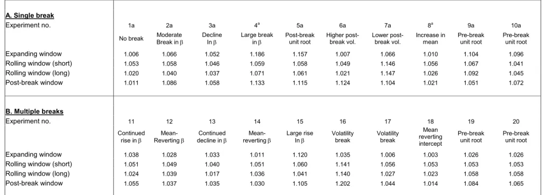
To shed light on the practical implications of our results, we next consider the out-of-sample forecasting performance of a range of widely used estimation windows. One way to deal with parameter instability is to use a rolling observation window. The size of the rolling window is often decided by a priori considerations. Here we consider a short rolling window using the most recent 25 observations and a relatively long rolling window based on the most recent 50 observations. If parameter instability is believed to be due to the presence of rare structural breaks, another possibility is to only use post-break data. In some cases the timing of the break may be known, but in most cases both the timing and the number of breaks must be estimated. We therefore use the Bai-Perron (1998) method to test for the presence of structural breaks and determine their timing, allowing up to three breaks and selecting the number of breaks by the Schwarz information criterion. If one or more breaks is identified at time t, this procedure uses data after the most recent break date to produce a forecast for periodt+ 1. If no break is identified, an expanding data window is used to generate the forecast. Finally, as a third option an expanding window is considered. This is the most efficient estimation method in the absence of breaks and provides a natural benchmark.
We initially undertook the following simulation exercise. For each of the orig-inal AR(1) experiments we assume a break has taken place at observation 101. Our post-break forecast evaluation period runs from observations 111 to 150. For this period we computed RMSFEs of the one-step ahead forecasts obtained under different estimation windows by Monte Carlo simulation.
Panel A of Table 6 reports the results under a single break. As expected, when a break is not present the expanding window method produces the lowest RMSFE
values. The expanding window also performs well when the break only affects the volatility or the mean parameter. The fact that the expanding window performs best even when the pre-break volatility is higher than the post-break volatility can be explained by the reduction in the variance of the parameter estimation error due to using a very long estimation window. The finding for a break in the mean is consistent with the simulation results in Table 4. In the experiments with a very large change in the autoregressive parameter (experiments 4-5), the short rolling window method produces the best performance, while the long rolling window works best for smaller breaks (experiments 2-3) which generate a lower squared bias.
Interestingly, the use of a post-break window with an estimated break point does not produce the lowest RMSFE performance in any of the experiments 1-8. A possible explanation of this finding lies in the modest power of break point tests to detect changes in autoregressive parameters as documented by Banerjee, Lumsdaine and Stock (1992). The only case where the post-break window method results in the lowest RMSFE is under a pre-break unit root (experiment 9). For this case the expanding window method performs quite poorly. This is consistent with our simulation results which showed that the conditional and unconditional RMSFE performance was best for very small - frequently zero - pre-break windows under a pre-break unit root. We also modified the simulation with the pre-break unit root to ensure that the point towards which the post-break process mean reverts is the terminal point of the pre-break unit root process (experiment 10) rather than simply µ2. This is likely to generate sample paths more similar to
those observed in practice, c.f. Banerjee, Lumsdaine and Stock (1992). The results show that although the expanding window method performs relatively better, it still does not produce the lowest RMSFE.
4.4. Multiple Breaks
So far we have focused on the case with a single structural break, but in practice the time series process under consideration may be subject to multiple breaks. Our procedure can readily be generalized to account for this possibility. Accordingly, we extended our simulation experiments to allow for two breaks occurring after 50 and 100 observations, respectively. The presence of multiple breaks raises questions concerning the process generating the breaks. Barring a general theory we consider
two scenarios. Thefirst scenario assumes that the two breaks lead to a shift in the regression coefficients in the same direction so for the AR(1) model we could have
β11 = 0.6, β12= 0.75 and β13= 0.9. The second scenario assumes mean reversion
in the parameters whichfirst shift away from their initial values (at thefirst break date) and then revert to their original values after the second break date, so we could have β11 = 0.6,β12 = 0.9 and β13 = 0.6. Further details of the assumed parameter values are reported in the note to Table 6.
The results, provided in Panel B of Table 6, suggest that the expanding window method continues to produce the lowest RMSFEs in a number of cases including those with breaks to the volatility parameter, breaks in the mean and mean re-version in the autoregressive coefficient. Mean-reversion across breaks in the au-toregressive coefficient tends to favor the expanding window method relative to the other methods since the earliest part of the sample will be similar to the final part from which the forecast is made. Adding the earliest part of the data sample prior to the first break therefore tends to pull the parameter estimate towards the value prevailing at the point of the forecast. In the few cases with multiple breaks where the expanding method does not dominate, the long rolling window method is generally best and it is frequently better to use a long rather than a short rolling window in the absence of a unit root.
5. Empirical Analysis
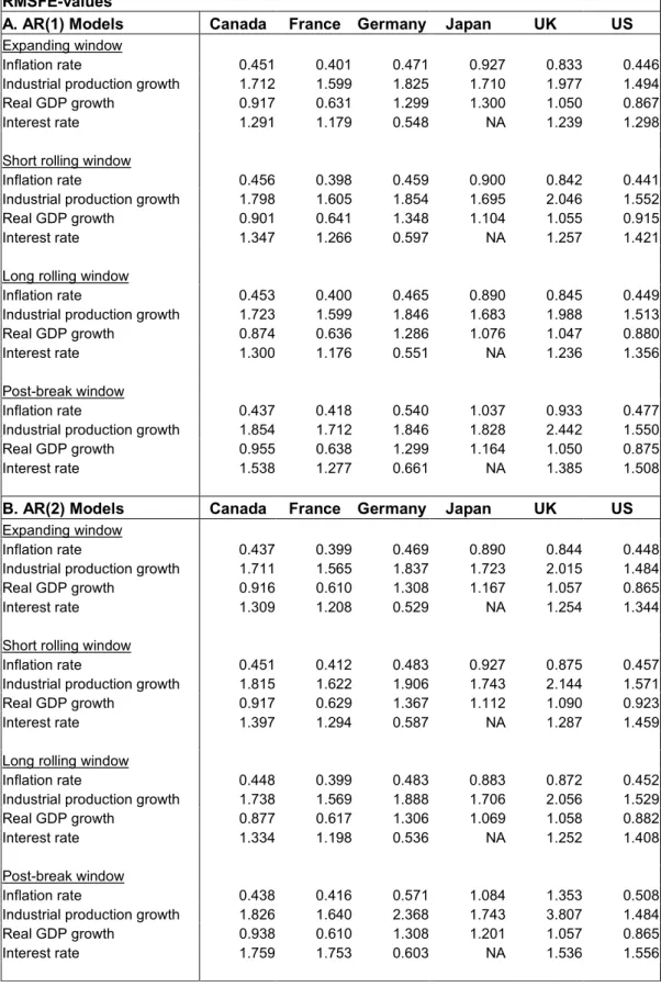
To better understand the practical implications of our theoretical analysis, we undertook a forecasting exercise using a range of macroeconomic time series. We considered forecasts of growth (log-first differences) in industrial production and real GDP, the inflation rate and short interest rates for six of the seven G7 countries, namely Canada, France, Germany, Japan, UK and the US. Italy was excluded due to incompleteness of data. All data is quarterly and covers the period 1959-1999. The data source is Stock and Watson (2003).
The forecasting exercise uses 25 initial observations for parameter estimation (or 40 observations in the case of the more heavily parameterized fourth order AR model) and considers AR(1), AR(2) and AR(4) models. All forecasts are out-of-sample and use data up to period t to estimate the parameters of a forecasting model that is then used to generate a forecast for period t + 1. The expanding window uses all available data up to timet. For the rolling windows we considered
short and long rolling windows that use the most recent 25 and 40 observations, respectively, corresponding to roughly six and ten years of data. We also consider the two-step post-break window method described earlier, where in the first step we use the Bai-Perron procedure to identify the break point nearest to the forecast date and in the second step only use post-break data to estimate the parameters of the forecasting model.
Table 7 reports the outcome of the empirical analysis. Panel A reports RMSFE-values for the four estimation windows assuming an AR(1) specification while panels B and C assume AR(2) and AR(4) models. For the AR(1) models the post-break estimation method only produces the lowest RMSFE values in one case (Canadian inflation) out of the total of 23 cases. This happens despite the fact that breaks are identified at some point in the majority of the series, i.e. for 21 of 23 series for the AR(1) model. The short rolling window method does marginally bet-ter than the post-break method, generating the lowest RMSFE values in three of 23 cases, while the long rolling window does best in seven cases. However, by some margin, the best method turns out to be the expanding window which generates the lowest RMSFE values in 12 cases.12
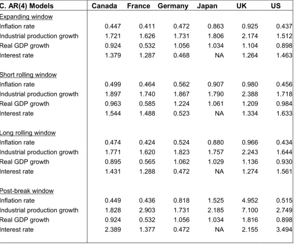
The results are even stronger for the AR(2) and AR(4) models. For the AR(2) case the expanding window produces the best forecasting performance in 17 out of 23 cases with the long rolling window doing best in the remaining six cases. The short rolling window and the post-break window never outperform these methods. Similarly, for the AR(4) model, the expanding window generates the lowest out-of-sample RMSFE values in 18 cases while the long rolling window does so in the remaining five cases.
The theory developed in this paper and our simulation results are very useful in understanding why it is difficult to reduce the RMSFE values produced by the expanding window method. For example, in the case of the AR(1) model, we found evidence for many of the variables either that the persistence of the series declined after the most recent break or - in cases with multiple breaks - that there was mean reversion in persistence across breaks. This would explain why the long rolling window generally performs better than the short rolling window.
12In some cases the forecasting performance of the post-break and expanding window method
is identical. This situation arises when no break point is detected so the full sample is used for estimation by the post-break method.
We also found that the 95% confidence interval for the time of the break fre-quently was quite wide and exceeded 10 observations. Imprecise determination of the time of the break can lead to a deterioration in the relative performance of the post-break forecasting method which will either be inefficient (if the estimated break date is later than the true date so that not all post-break data is used) or biased (if the estimated break date is premature so pre-break observations get in-cluded in the estimation window). In many cases the post-break window was also rather short, only averaging between one-half and one-third of the length of the expanding window, leading to imprecisely estimated values of the parameters of the forecasting model.
A final reason for the better overall performance of the expanding window estimation method over the other methods lies in the empirical importance of breaks to the innovation variance, σ2. Experiments 6, 7, 16 and 17 in Table 6
showed that the expanding window method tends to be best under a volatility-only break. This finding is likely to carry over to cases with breaks in other parameters provided that the break in the volatility parameter is large relative to breaks in the other parameters. Indeed, we often observed very large variations in the estimates of σ across different break segments.
Overall, our results suggest that the squared bias arising from using pre-break data in estimation of the parameters of autoregressive forecasting models subject to breaks is less important to forecasting performance than the variance of the parameter estimation error. This would also explain the improved performance of the methods that use the longest estimation windows under the higher order AR models compared to theAR(1) model since these models require estimation of more parameters.
Another interesting finding emerging from Table 7 is that, in general, variation in the out-of-sample RMSFE is greater across the various estimation windows than it is across the lag order chosen for the autoregressive model estimated through the expanding window method. A large amount of work has gone into designing meth-ods for lag order selection. Our results suggest that the forecasting performance of autoregressive models subject to breaks could be even more affected by the length of the estimation window than by the autoregressive order and that a post-break estimation method - albeit appealing in theory - is difficult to implement success-fully in practice for dynamic models. This points to the practical importance of
gaining a better understanding of how to best determine the length of the data window used to estimate the parameters of the forecasting model.
6. Conclusion
This paper studied the small sample properties of forecasts from autoregressive models subject to breaks. It is insightful to compare and contrast our results for the AR(p) model to those reported by Pesaran and Timmermann (2003) under strictly exogenous regressors. Assuming strictly exogenous regressors, the OLS estimates based on post-break data are unbiased. Including pre-break data will therefore always increase the bias so that there will always be a trade-off between a larger squared bias and a smaller variance of the parameter estimates as more pre-break information is used. This trade-off can then be used to optimally determine the window size.
As we have shown in this paper, the situation can be very different for AR models due to the inherent small-sample bias in the estimates of the parameters of these models. In situations where the true AR coefficient(s) declines after a break, both the bias and the forecast error variance can in fact be reduced as a result of using pre-break data in the estimation. This is likely to be an important reason why, empirically, it is often difficult to improve forecasting performance over the expanding or long rolling window methods by only using post-break data. It also explains why forecasts based on a rolling window often perform worse than forecasts based on an expanding window of the data, particularly in cases where a short rolling window is used. These observations were confirmed empirically in an analysis of forecasts of GDP and industrial production growth, inflation and interest rates for six major economies.
More generally, we find both theoretically and empirically that there are many scenarios where the inclusion of some pre-break data for purposes of estimation of the parameters of autoregressive models leads to lower biases and lower mean squared forecast errors than if only post-break data is used. This can hold even when the post-break window is large, particularly when the post-break data gener-ating process is highly persistent and/or has a break in the mean or variance. Our
findings also indicate the possibility of a hybrid method that starts with an expand-ing window if the data set is relatively short and then switches to a long rollexpand-ing window as the data set grows beyond a pre-specified threshold. We are currently
investigating into the possible ways that such a threshold could be determined. Several extensions to our results would be interesting to consider in future work. We have focused on the case with Gaussian innovations. Ullah (2003) observes that the bias in the forecast error is reasonably robust to skewness and kurtosis in the innovations of the AR model while, in contrast, the mean squared forecast error can be sensitive to higher order moments that arise in the non-Gaussian case. Our results could easily be extended to cover the non-normal case, for example by drawing innovations from a mixture of normals. Other possibilities are to consider the effect of additional predictors beyond autoregressive lags, multi-step ahead forecasts, and forecasts from vector autoregressive processes with or without cointegrating restrictions. Our theoretical and simulation results suggest that the empirical dominance of the expanding or long rolling window estimation method documented in this paper for univariate autoregressive models is likely to hold in these more complicated settings.
Bibliography
Abadir, K.M., 1993, OLS bias in a nonstationary autoregression. Econometric Theory 9, 81-93.
Alogoskoufis, G.S. and R. Smith, 1991, The Phillips Curve, the Persistence of Inflation, and the Lucas Critique: Evidence from Exchange Rate Regimes. Amer-ican Economic Review 81, 1254-1275.
Andrews, D.W.K., 1993, Tests for Parameter Instability and Structural Change with Unknown Change Point. Econometrica 61, 821-856.
Andrews, D.W.K. and W. Ploberger, 1996, Optimal Changepoint Tests for Normal Linear Regression. Journal of Econometrics 70, 9-38.
Bai, J. and P. Perron, 1998, Estimating and Testing Linear Models with Mul-tiple Structural Changes. Econometrica 66, 47-78.
Bai, J. and P. Perron, 2003, Computation and Analysis of Multiple Structural Change Models, Journal of Applied Econometrics, 18, pp. 1-22.
Banerjee, A., J.J. Dolado, D.F. Hendry and G.W. Smith, 1986, Exploring equi-librium relationships in economics through static models: some Monte Carlo evi-dence. Oxford Bulletin of Economics and Statistics 48, 253-277.
Banerjee, A., R. Lumsdaine and J.H. Stock, 1992, Recursive and Sequential Tests of the Unit-Root and Trend-Break Hypotheses: Theory and International Evidence. Journal of Business and Economic Statistics 10, 271-287.
Bartlett, M.S., 1946, On the theoretical specification and sampling properties of autocorrelated time series. Supplement to the Journal of the Royal Statistical Society 8, 27-41.
Box, G.E.P. and G.M. Jenkins, 1970, Time Series analysis: forecasting and control. San Francisco: Holden Day.
Chong, T. T-L, 2001, Structural Change in AR(1) Models. Econometric Theory 17(1), 87-155.
Chu, C-S J., M. Stinchcombe, and H. White, 1996, Monitoring Structural Change. Econometrica 64, 1045-1065.
Clements, M.P. and D.F. Hendry, 1998, Forecasting Economic Time Series. Cambridge University Press.
Clements, M.P. and D.F. Hendry, 1999, Forecasting Non-stationary Economic Time Series. The MIT Press.
Copas, J.B., 1966, Monte Carlo results for estimation in a stable Markov time series. Journal of the Royal Statistical Society 129, 110-116.
Elliott, G. and U. Muller, 2002, Optimally Testing General Breaking Processes in Linear Time Series. Manuscript, UCSD and Princeton University.
Evans, G.B.A. and N.E. Savin, 1981, Testing unit roots: 1. Econometrica 49, 753-779.
Fuller, W.A, 1996, Introduction to Statistical Time Series. John Wiley & Sons, Inc.
Fuller, W.A. and D.P. Hasza, 1981, Properties of predictors for autoregressive time series. Journal of the American Statistical Association 76, 155-161.
Garcia, R. and P. Perron, 1996, An Analysis of the Real Interest Rate under Regime Shifts. Review of Economics and Statistics 78, 111-125.
Giacomini, R., 2002, Tests of Conditional Predictive Ability. Manuscript UCSD. Grubb, D., Symons, J., 1987. Bias in regressions with a lagged dependent variable. Econometric Theory 3, 371-386.
Hansen, B.E., 1992, Tests for Parameter Instability in Regressions with I(1) Processes. Journal of Business and Economic Statistics 10, 321-335.
Ret-rospective Detection of Changes of Variance. Journal of the American Statistical Association 89, 913-923.
Kiviet, J.F., Phillips, G.D.A., 1993, Alternative bias approximations in regres-sions with a lagged dependent variable. Econometric Theory 9, 62-80.
Kiviet, J., and Phillips, G.D.A., 2003a, Improved Coefficient and Variance Es-timation in Stable First-Order Dynamic Regression Models, UvA-Econometrics discussion paper 2002/02, version March 2003.
Kiviet, J., and Phillips, G.D.A., 2003b, Moment Approximation for Least Squares Estimators in Dynamic Regression Models with a Unit Root, version April 2003, UvA-Econometrics discussion paper 2003/03.
Pesaran, M.H. and A. Timmermann, 2002, Market timing and return prediction under model instability. Journal of Empirical Finance, 9, 495-510.
Pesaran, M.H. and A. Timmermann, 2003, Window selection with strictly ex-ogenous regressors. Unpublished manuscript University of Cambridge and UCSD. Phillips, P.C.B., 1977, Approximations to somefinite sample distributions asso-ciated with a first-order stochastic difference equation. Econometrica 45, 463-485. Phillips, P.C.B., 1987, Asymptotic expansions in nonstationary vector autore-gression. Econometric Theory 3, 45-68.
Ploberger, W., W. Kramer, and K. Kontrus, 1989, A New Test for Structural Stability in the Linear Regression Model. Journal of Econometrics 40, 307-318.
Sawa, T., 1978, The exact moments of the least squares estimator of the au-toregressive model. Journal of Econometrics 8, 159-172.
Smith M.D., 1988, Convergent series expressions for inverse moments of quadratic forms in normal variables, Australian Journal of Statistics, 30, 235-246.
Stock, J.H., 1987, Asymptotic properties of least squares estimators of cointe-grating vectors. Econometrica 55, 1035-1056.
Stock, J.H. and M.W. Watson, 1996, Evidence on Structural Instability in Macroeconomic Time Series Relations. Journal of Business and Economic Sta-tistics 14, 11-30.
Stock, J.H. and M.W. Watson, 1999, A Comparison of Linear and Nonlinear Univariate Models for Forecasting Macroeconomic Time Series. Chapter 1 of En-gle, R.F. and H. White (1999), Cointegration, Causality and Forecasting. Oxford University Press.
in a Seven-Country Data Set. Harvard University mimeo.
Ullah, A., 2003, Finite sample econometrics. Manuscript, University of Califor-nia, Riverside.
Appendix A: Distribution of the Initial Values when the
Pre-Break Process is I(1)
For the AR(2) case we first note that
ym−2 = y1+∆y2+...+∆ym−2,
ym−1 = y1+∆y2+...+∆ym−2+∆ym−1. (37)
This provides a decomposition ofym−i,i= 1,2 in terms of the non-stationary level
component, y1, and stationary first differences, ∆y2,∆y3, .... The distribution of
(ym−2, ym−1) can now be derived for given assumptions concerning y1 and ∆y2.
There are many possibilities. As a simple example we consider the situation where as in the AR(1) casey1 ∼N(µ1,ω2) is distributed independently of∆yt, t= 2,3, ..,
and assume that the stationary components of ym−2 and ym−1 are started with ∆y1 = 0. Under these assumptions we have y1 =ωε1 and ∆y2 = σ1ε2 and, using
(13),
∆yt=δ11∆yt−1+σ1εt, t= 3,4, ..., T1,
where |δ11|<1, thus ensuring that yt ∼I(1). Using these relations we have
∆y2 = σ1ε2 ∆y3 = δ11σ1ε2+σ1ε3 .. . ∆ym−2 = δm11−4σ1ε2 +δ m−5 11 σ1ε3+...+δ11σ1εm−3+σ1εm−2 ∆ym−1 = δm11−3σ1ε2 +δ m−4 11 σ1ε3+...+δ 2 11σ1εm−3+δ11σ1εm−2 +σ1εm−1
Substituting these in (37) we now have
ym−2 = y1+ σ1ε2¡1−δm11−3 ¢ 1−δ11 + σ1ε3¡1−δm11−4 ¢ 1−δ11 +...+ σ1εm−2(1−δ11) 1−δ11 ym−1 = y1+ σ1ε2¡1−δm11−2¢ 1−δ11 + σ1ε3¡1−δm11−3¢ 1−δ11 +... σ1εm−2 ¡ 1−δ211¢ 1−δ11 + σ1εm−1(1−δ11) 1−δ11 .