Does Opportunism Pay Off?

Full text

(1)“Does Opportunism Pay Off?” Linda Gonçalves Veiga Francisco José Veiga NIPE WP 5 / 2006.

(2) “Does Opportunism Pay Off?” Linda Gonçalves Veiga Francisco José Veiga. NIPE* WP 5 / 2006. URL: http://www.eeg.uminho.pt/economia/nipe/documentostrabalho.php *. NIPE – Núcleo de Investigação em Políticas Económicas – is supported by the Portuguese Foundation for Science and Technology through the Programa Operacional Ciência, Teconologia e Inovação (POCTI) of the Quadro Comunitário de Apoio III, which is financed by FEDER and Portuguese funds..

(3) Does Opportunism Pay Off? * Linda Gonçalves Veiga Núcleo de Investigação em Políticas Económicas Universidade do Minho P-4710-057 Braga – Portugal Tel.: +351-253-604568 Fax: +351-253-676375 E-mail: [email protected] Francisco José Veiga Núcleo de Investigação em Políticas Económicas Universidade do Minho P-4710-057 Braga – Portugal Tel.: +351-253-604534 Fax: +351-253-676375 E-mail: [email protected]. Abstract: This article tests the hypothesis that the opportunistic manipulation of financial accounts by mayors increases their chances of re-election. Working with a large and detailed dataset comprising all Portuguese mainland municipalities, which covers the municipal elections that took place from 1979 to 2001, we clearly show that increases in investment expenditures and changes in the composition of spending favouring highly visible items are associated with higher vote percentages for incumbent mayors seeking re-election. Our results also indicate that the political payoff to opportunistic spending increased after democracy became well-established in the country.. Keywords: Voting functions, opportunism, local governments, elections, Portugal. JEL codes: D72, H72. *. The authors wish to thank Henry Chappel for very helpful comments and the Portuguese Foundation for Science and Technology (FCT) for funding the project “Interactions between economics and politics in Portugal” under research grant POCI/EGE/58641/2004 (partially funded by FEDER)..

(4) 1. Introduction The objective of the present article is to determine whether opportunistic mayors can increase their chances of re-election by generating political business cycles around elections. We test the hypothesis that pre-electoral increases in municipal expenditures and changes in their composition, favouring items most visible to or preferred by the electorate, are associated with higher vote percentages for the incumbent mayor. Research is conducted over a dataset comprising all the Portuguese mainland municipalities, from 1979 to 2001. In previous work, Veiga and Veiga (2004c) found strong evidence of political budgetary cycles in Portuguese municipalities. Their analysis reveals that deficits, and expenditures, particularly investment, increase significantly in election years and, in some cases, in the year before. They also showed that electoral cycles were stronger for investment items highly visible to the electorate, for example, construction spending on public infra-structure. Given these results, it would also be interesting to investigate: (1) if voters reward politicians’ opportunistic spending policies, or punish them, as suggested by Peltzman (1992); (2) if the items targeted by mayors’ electoral policies are those that generate more votes. Additionally, because democracy was reestablished in Portugal in 1974, during our sample period the country has evolved from a “new” to an “established” democracy. This makes Portugal an appropriate laboratory for analyzing if the determinants of electoral results change as a democracy matures. In the article, we also test if the popularity of the national government conditions local electoral results, and whether time in office decreases incumbents’ popularity. The international literature on vote and popularity functions is already quite extensive (Paldam, 2004). However, most of the research concentrates on national governments and the Portuguese case is clearly under researched. At the local level,. 1.

(5) there is only Costa (1998), who analysed the 1989 and 1993 municipal elections. At the national level, Veiga and Veiga (2004a), and Veiga and Veiga (2004b) estimate, respectively, popularity functions for the four main Portuguese political entities and vote intentions functions for the main political parties in the country. Use of data for Portuguese municipalities is also motivated by the following reasons. First, we have very detailed data on local governments’ financial accounts. Second, the mayor is a principal decision-maker in the allocation of resources and the distribution of investment in the municipality. Third, the institutional structure of local governments and the policy instruments available are the same for all localities, making this panel preferable to one composed of several countries. Finally, election dates are fixed and defined exogenously from the perspective of the local authorities, and all municipalities have elections on the same day. This article is organized as follows. The next section presents some background information on Portuguese municipalities. Section 3 describes the data sources and section 4 the empirical model. Results are discussed in section 5. Finally, section 6 reports the conclusions.. 2. Portuguese municipalities: brief characterization This. section. presents. some. background. information. on. Portuguese. municipalities. Democracy was re-established in Portugal by the bloodless military coup of April 25, 1974, which put an end to 48 years of dictatorship. Portuguese municipalities were formally established in the Constitution of 1976 and the first municipal elections took place in December of the same year. Portuguese local governments are responsible for improving their populations’ well-being, promoting social and economic development, territory organization, and for supplying local public. 2.

(6) goods (water and sewage, energy, transportation, housing, healthcare, education, culture, sports, defence of the environment, and protection of the civilian population).1 The representative branches of municipalities’ government are the Town Council and the Municipal Assembly2. The members of the Town Council are elected directly by voters registered in the municipality, who vote for party or independent lists. Votes are then transformed into mandates using the Hondt method, and the mayor is the first candidate from the list that receives the most votes. Part of the Municipal Assembly is elected directly by voters while the remaining members are the presidents of the councils of the freguesias that belong to the municipality.3 The Municipal Assembly approves the general framework for local policies, while the Town Council, which holds the executive power, is responsible for its elaboration and implementation. The mayor is the president of the Town Council and has a prominent role in the executive. Budgeting rules and institutions are the same for all Portuguese mainland municipalities, although the law regulating local public finances changed during the period considered.4 Municipalities are financially autonomous. They have their own employees and assets, and they define the local budget and the plan of activities without a requirement of authorization from a higher-ranked authority. As part of the general government sector, local authorities are, however, subject to several control mechanisms by central government agencies. These limit their access to revenues as well as their expenditure choices. It is worth noting that election dates are defined exogenously from the perspective of the local authorities and that during our sample period there was no legal restriction to the number of terms a mayor could stand for re-election. Since the re1. Law 159/99 defines the areas of intervention of Portuguese local governments. Law 169/99 establishes the competencies and the legal framework of municipalities’ branches. 3 Freguesias are subdivisions of municipalities. They are the lowest administrative unit in Portugal. 4 Law 1/79, Decree-Law 98/84, Law 1/87 and, currently, Law 42/98. 2. 3.

(7) establishment of Democracy in 1974, there were local elections in December of 1976, 1979, 1982, 1985, 1989, 1993, 1997 and 2001, and in October 2005.. 3. Data sources The dataset is composed of data on a set of political, financial and economic variables for the 278 Portuguese mainland municipalities. Due to the restrictions imposed by data availability, the election years covered in this study are 1979, 1982, 1985, 1989, 1993, 1997 and 2001.5 Since this article tries to determine whether or not political opportunism of mayors pays off, only the cases in which they run for reelection are considered. Political data, namely election dates and municipal electoral results, were obtained from the National Electoral Commission (Comissão Nacional de Eleições) and from the Technical Staff for Matters Concerning the Electoral Process (Secretariado Técnico dos Assuntos para o Processo Eleitoral) of the Internal Affairs Ministry. The government popularity index is based on the monthly surveys published in the newspaper Expresso, from 1986 to 2001. Data on municipal local accounts and population were obtained from the local authority’s (Direcção Geral das Autarquias Locais) annual publication called Finanças Municipais (Municipal Finances). This report exists from 1979 to 1983 and from 1986 to 2002. For the two missing years data was obtained directly from the municipalities’ official accounts and are incomplete: we have 182 observations for 1984 and 189 for 1985. Consumer price indexes were taken from the OECD’s Main Economic Indicators. Data on the total number of employees in firms within each municipality and on their average wages, from 1985 to 2000, was obtained from the “Quadros de Pessoal” 5. Although there was also an election in October 2005, data on the municipal financial accounts is only available until 2003. The election of 1979 is not covered in several estimations (whenever lags, term means or deviations from term means are included).. 4.

(8) database, of the Portuguese Ministry of Labour and Social Solidarity (MTSS).6 Finally, data on the Municipal Purchasing Power Index, for the years 1993, 1995, 1997, 2000, 2002 and 2004 was obtained from the National Statistics Office (INE).. 4. Specification of the empirical model The empirical models to be estimated for a panel of 2757 municipalities, over a maximum of seven elections, use the percentage of votes obtained by the incumbent in the current elections, Votes, as the dependent variable. In the set of explanatory variables, we start by including the percentage of votes obtained by the incumbent in the previous balloting, Votes (Previous Election).8 This variable accounts for the support the mayor enjoyed at the start of the term and for factors not considered in the other explanatory variables, such as the mayor’s personal characteristics, ideology and party affiliation of voters, socio-economic characteristics of each municipality, etc. The erosion of the mayor’s popularity as he/she stays longer in power is accounted for by including a variable, Years President, that counts the number of years during which the incumbent has remained in power (a negative estimated coefficient is expected for this variable). Mayors’ popularity tends to decrease with time in office because the policy actions, even if supported by most of the electorate, will tend to alienate some voters, who will then support the opposition (Mueller, 1970, and Frey and Schneider, 1978). Voter support may also decay when mayors fail to deliver what they promised during the electoral campaigns (Mueller, 1970). 6. The “Quadros de Pessoal” is a yearly mandatory employment survey that covers virtually all privately owned firms employing paid labor in Portugal (public servants and own employment are not included). Although the most recent year for which data is available is 2003, there is no data on wages for 2001. 7 For the three municipalities created in 1997 (Odivelas, Trofa and Vizela) there is only election data for 2001 (the last election in our sample), which means that there is no data for the votes obtained in the previous elections. Thus, in the estimations, we have a maximum of 275 municipalities. 8 It is worth mentioning that Votes (Previous Election) is not always equal to the first lag of Votes. That only happens in municipalities in which the mayor was always reelected. In fact, the correlation between Votes (Previous Election) and lagged Votes is around 75%.. 5.

(9) It is also possible that the votes for an incumbent mayor whose political party is in charge of the national government are affected by the popularity of the latter. That is, the electorate may also wish to reward, or punish, the national government in second order elections. Carsey and Wright (1998, p. 995) formulate this possibility in the following manner for the United States: “For many citizens, political judgements are general indictments or rewards of the party in power, usually defined as the presidential party. Thus, we expect presidential approval to influence all types of subpresidential voting behaviour.” We account for this possibility with an interaction variable that consists in multiplying the dummy variable Government’s Party (that takes the value of one when the mayor’s party is that of the Prime Minister, and equals zero otherwise) by the value of the Government Popularity Index in the month of the elections.9 Since a more popular government may help the mayors of the same party getting higher percentages of votes, a positive coefficient is expected for Government’s Party*Government Popularity. One problem with this variable is that it leads to many missing values, as the popularity data is only available from 1986 onwards. In order to be able to work with data since 1979, another interaction variable was created, which consists in multiplying the dummy variable Government’s Party by the national Inflation Rate. Since voters tend to punish the national government for bad economic outcomes,10 higher inflation should lead to lower percentages of votes for the incumbent mayors of the government’s party (a negative coefficient is expected for this interaction variable).. 9. See Veiga and Veiga (2004a) for the definition of the index and for graphs that illustrate its evolution. On the responsibility hypothesis and for a survey of the vote/popularity functions literature, see Paldam (2004). For evidence on the Portuguese case, at the national level, see Veiga and Veiga (2004a and 2004b).. 10. 6.

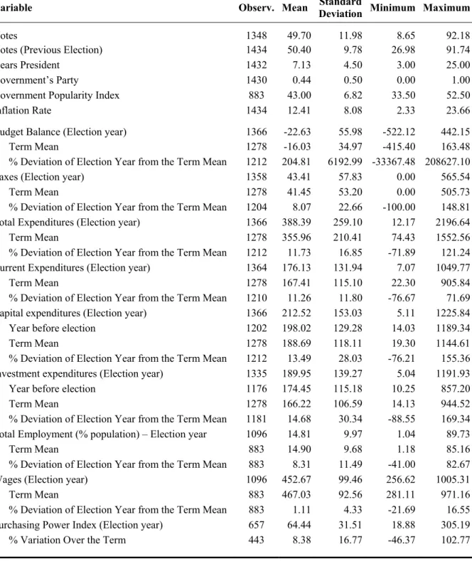
(10) The first group of tests of the hypothesis that opportunism pays off use data on more aggregated accounts, such as budget balances, taxes and total expenditures. We then test the hypothesis using more detailed data. First, we split expenditures into current and capital. Second, we estimate models for total investment expenditures (the main component of capital expenditures). Finally, its components and sub-components are also analysed. This very detailed analysis, that considers all types of investment expenditures, allows for the identification of those for which pre-electoral manipulation would increase the percentage of votes for the incumbent. That is, we are able to identify the types of expenditures that opportunistic mayors should target and to check whether or not they correspond to those for which Veiga and Veiga (2004c) found evidence of political business cycles. Ultimately, votes should be driven by the incumbent’s performance and not necessarily by the magnitude or the composition of expenditures. Since there is no data on the quality of the services provided by the Portuguese municipalities, we use the few measures of municipal economic performance that are available. Thus, the final step of the empirical analysis is to control for the evolution of employment,11 wages and purchasing power in each municipality. Descriptive statistics for all the variables mentioned above are presented in Table 1.12 [Insert Table 1 about here] Two empirical models will be estimated in order to check if opportunism pays off. In the first, the levels of the variables that may be the object of opportunism in the election year and in the two previous years are included along with the political variables referred to above. The empirical model can be specified as follows: 11. See Coelho, Veiga and Veiga (forthcoming) for a study of political business cycles in municipal employment. 12 The descriptive statistics for the components and sub-components of investment expenditures were not included in order to economize space, but they are available from the authors upon request.. 7.

(11) Votesit = αVotesi , prev.el . + φYPit + γGPit + X it' β1 + X i' ,t −1β 2 + X i' ,t − 2 β 3 + ν i + ε it. i = 1,...,275. t = 1979,1982,1985,1989,1993,1997, 2001. (1). where Votesit is the percentage of votes obtained by the incumbent’s party in the election of year t, Votesi,prev.el. is the percentage of votes obtained in the previous election, YPit stands for Years President and GPit stands for Government’s Party*Inflation Rate or for Government’s Party*Government Popularity, X is a vector of variables subject to opportunistic manipulation (their levels in the election year, t; the year before elections, t-1; and two years before elections, t-2, are included),13 νi is the individual effect of municipality i, εit is the error term, α, φ and γ are parameters and β1, β2 and β3 are vectors of parameters to be estimated. Evidence that opportunism pays off would be consistent with a positive and statistically significant β1, eventually, a positive and statistically significant β2, and a negative or statistically insignificant β3. The second model uses the term mean and the percentage deviation of the level in the election year relative to the term mean of the variables included in vector X. The empirical model can be specified as follows: Votes it = αVotes i , prev.el . + φYPit + γGPit + Xtm it' β1 + Xdev i' ,t β 2 + ν i + ε it. i = 1,...,275. t = 1979,1982,1985,1989,1993,1997, 2001. (2). where Xtm is a vector of term means of the variables included in X, Xdev is a vector of the percentage deviations of their election year values from the term means, and all the remaining variables and parameters are defined as in equation (1). Evidence that opportunism pays off would be consistent with a positive and statistically significant β2.. 13. Since the first terms were only three-years long, when working with the full sample it is not possible to include the level of X three years before elections, because in those cases it would be an election year. That value will be included when working just with the most recent elections.. 8.

(12) A positive and statistically significant β1 means that greater average values of the X variables over a term are associated with greater percentages of votes.. 5. Empirical results. The estimation results of the panel data models described in the previous section, controlling for municipality fixed effects,14 are shown in Table 2.15 T-statistics are presented between parentheses and the degree of statistical significance is signalled with asterisks. The number of observations, municipalities and elections, and the adjusted R squared are reported at the foot of the table. In column 1 of Table 2, we report the results of the estimation of the model of equation (1) for three variables which may be subject to opportunistic manipulation by mayors: the municipal Budget Balance, Taxes, and Total Expenditures.16 Although Veiga and Veiga (2004c) found evidence of political business cycles in these three variables, none of them seems to have a positive and statistically significant effect on the votes obtained.17 As expected, Votes (Previous Election) has a positive sign and is statistically significant, indicating that there is some persistence in vote shares. There is also evidence of popularity erosion over time, as Years President is statistically significant with a negative sign. The same result is obtained for Government’s. 14. Municipal dummy variables are globally statistically significant, and Hausman tests indicate that a fixed effects specification is always preferable to a random effects one. 15 As explained above, Votes (Previous Election) is not the first lag of Votes (their correlation is around 75%). Thus, the implementation of the Arellano and Bond (1991) difference GMM estimator for linear dynamic panel data models would not be appropriate. Nevertheless, we estimated it just as a robustness check, and the results (available upon request) were similar to those presented in this paper. 16 For each municipality, all fiscal variables were divided by the consumer price index for the base year (1995) and, then, by its population. Thus, they are expressed in euros (of 1995) per capita. The budget balance, based on public accounting, is calculated according to the methodology of the General Direction of the Budget (Direcção Geral do Orçamento) of the Ministry of Finance, which excludes the transactions in financial assets and liabilities from the totals of revenues and expenditures. 17 As indicated in equation (1), we started with the estimation of a model which also included the values of the three fiscal variables one and two years before the elections. Then, these lagged values were sequentially excluded from the model when they turned out not statistically significant.. 9.

(13) Party*Inflation Rate, indicating that when inflation is high, mayors that belong to the prime minister’s party tend to lose votes. [Insert Table 2 about here]. The results of the estimation of the model of equation (2) are reported in column 2. Again, there is no evidence that the manipulation of the Budget Balance or of Taxes affects votes. Concerning Total Expenditures, their Term Mean is positive and statistically significant, meaning that mayors who have higher average expenditures over the term tend to get more votes. But, spending relatively more in the election year does not seem to result in higher vote shares, as the % Deviation of the Election Year from the Term Mean is not statistically significant. In the estimations of columns 3 and 4, the dummy variable Government’s Party was interacted with Government Popularity instead of with the inflation rate. As expected, this interaction variable is statistically significant, with a positive sign. Now, Total Expenditures in the election year are highly statistically significant (column 3), indicating that greater expenditures lead to higher percentages of votes.18 The difference of results when comparing to those of column 1 may be explained by the fact that in the estimation of column 3 only the last 4 elections are considered, while that of column 1 considers all 7 elections that took place during the sample period.19 In order to study the possibility that opportunism worked better in the most recent elections, the sample was split in two: one sub-sample covers the first four elections (1979, 1982, 1985 and 1989), while the other covers the last three elections (1993, 1997 and 2001). Results of columns 5 and 6 imply that opportunism did not. 18. When including the levels of expenditures for the election year and for previous years only the one for the election year is statistically significant. When including one at a time, the level for the election year has the highest t-ratio. This result confirms the evidence for voter myopia found in the vote/popularity functions literature (see Paldam, 2004). 19 Results for the term average of Total Expenditures may be stronger in column 4 than in column 2 for the same reason.. 10.

(14) work in the period 1979-1989, as the fiscal variables are never statistically significant.20 In the period 1990-2001, the opportunistic manipulation of Total Expenditures seems to have worked well. Expenditures in the election year are positively related to votes (columns 7 and 9), with 90 to 100 euros per capita of additional expenditures resulting in an increase of one percentage point in the vote share. In columns 8 and 10, both the term mean expenditures and the percentage deviation of election year expenditures from the term mean are positive and statistically significant. This implies that for a mayor it is both worthwhile to spend more on average over the term, and to increase expenditures in the election year relative to the previous years of the same electoral cycle.21 The fact that opportunism paid off better in the most recent Portuguese municipal elections contradicts the results of Brender and Drazen (2005) that indicate that political business cycles tend to work in new democracies but not in established ones. That is, our results imply that they worked better as the Portuguese democracy became more established (1990-2001) than in the first elections after the restoration of democracy in 1974. A possible explanation for this result is that, as democracy matured, not only voters learned about the democratic system; politicians may also have acquired more knowledge on how to implement electoral politics. It is worth mentioning that according to Alt and Lassen (2006), conditioning on the degree of fiscal policy transparency, electoral cycles also exist in advanced industrialized economies. Therefore, in line with Rogoff and Sibert (1988) and Rogoff (1990) models of rational opportunistic budget cycles, our result suggest that, even in the latter years of 20. Since the data on the government’s popularity only starts in 1986, it is not possible to include it in the estimations for the period 1979-1989. 21 Concerning political variables, results are similar across the sub-samples, except for Government’s Party*Inflation Rate, which has a positive sign in 1993-2001, and is marginally statistically significant. That change in the sign may be due to the fact that inflation was no longer a major economic problem by the time of the elections of 1997 and 2001, as it reached low levels comparable to those of the other EU members.. 11.

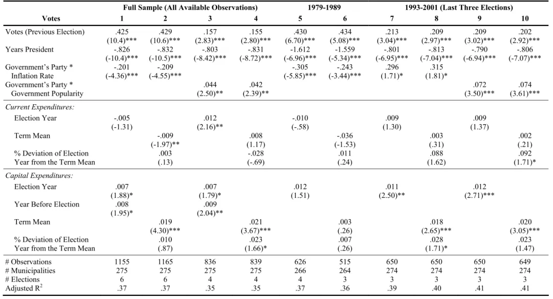
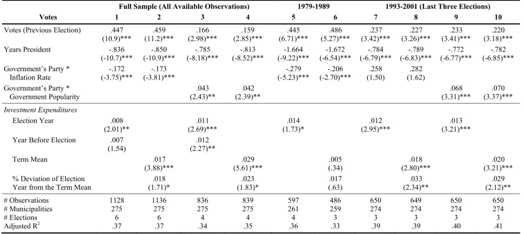
(15) democracy, there is asymmetry of information between voters and politicians, that the latter explore by manipulating budgetary items in order to increase their chances of reelection. The next step of the analysis was to determine which type of expenditures produced greater effects on votes. For that purpose, Current and Capital Expenditures were considered in the models of Table 3. It is worth mentioning that, when considering more than on type of expenditures, opportunism can take two forms: increased expenditures in the election year; and, strategic changes in the composition of expenditures favouring the type(s) most preferred by the electorate.22 [Insert Table 3 about here]. The coefficients associated with Current Expenditures are generally not statistically significant, which means that its opportunistic manipulation does not tend to increase votes (the exceptions are columns 3 and 10). Results for Capital Expenditures are similar to those obtained for Total Expenditures in Table 2. The main difference is that expenditures in the Election Year and in the Year Before Election are also significant in column 1. Thus, there is evidence that higher Capital Expenditures prior to elections help gaining votes and that it also would pay off to strategically shift funds from Current to Capital Expenditures.23 Since Investment Expenditures account on average for almost 90% of Capital Expenditures, and are their most visible component to voters, it is likely that this is the type of expenditures that has greater impact on votes. In fact, results for Investment Expenditures, presented in Table 4, are stronger than those for Capital Expenditures shown in Table 3: t-statistics are generally higher, the % Deviation of the Election Year. 22. See Drazen and Eslava (2005) for a theoretical model on opportunism via expenditure composition. A similar result was obtained by Drazen and Eslava (2005) for Colombian municipalities. A result indicating that it may be worth increasing expenditures of both types is that of column 3.. 23. 12.

(16) from the Term Mean is now also statistically significant for the full sample (column 2), and the expenditures in the Election Year are marginally significant in the period 19791989 (column 5). These stronger effects of Investment Expenditures on votes are consistent with the results of Veiga and Veiga (2004c), who found evidence of greater political business cycles in that type of expenditures than in the other fiscal items analysed.24 [Insert Table 4 about here]. In the estimations of Table 5, investment expenditures are broken up into their seven components. In column 1, only Other Buildings and Miscellaneous Constructions are statistically significant. These results, confirmed in column 3 where only these two components are considered, were somewhat expected, as these are the most important and most visible components of Investment Expenditures. Although estimation results shown in column 2 only present evidence that opportunism pays off for Other Buildings, and eventually for Other Investments, those of column 4 show that is also worthwhile to spend more on average in Miscellaneous Constructions. Thus, an opportunistic mayor can gain votes by strategically shifting funds from the five components of Investment Expenditures that are not statistically significant into Other Buildings and/or Miscellaneous Constructions.25 [Insert Table 5 about here]. Since we have very detailed data on the municipal accounts, we are able to disaggregate Investment Expenditures even further, in order to analyse the three components of Other Buildings and the six components of Miscellaneous. 24. Using data only for the municipal elections of 1989 and 1993, Costa (1998) found out that investment expenditures had a positive effect on votes, while current expenditures, such as disbursements to compensation of employees, seemed to have no effects. 25 In order to economize space, only the results obtained when using Government’s Party*Inflation Rate (the one for which the number of observations is higher) are shown in Tables 5 and 6. Results when using Government’s Party*Government Popularity are very similar (they are available upon request). 13.

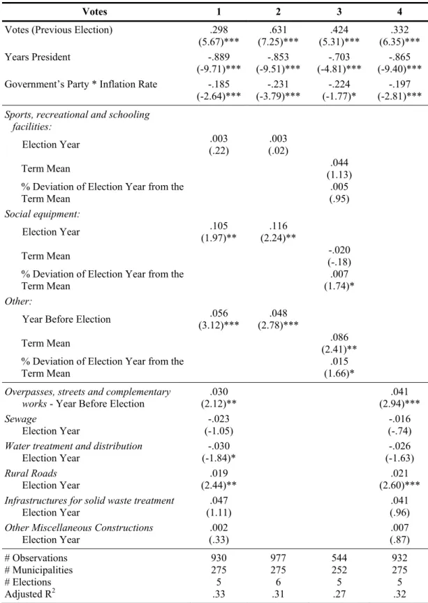
(17) Constructions. The results of the estimation of the model of equation (1) for these nine sub-components of Investment Expenditures are shown in column 1 of Table 6. These indicate that votes can be gained by increasing expenditures in the election year (or in the year before, in some cases) in Social Equipment, Other, Overpasses, streets and complementary works, and in Rural roads. In columns 2 and 3, where only the components of Other Buildings are considered, evidence that opportunism pays off is confirmed for Social Equipment and Other. Finally, the results of column 4, for a model including only the components of Miscellaneous Constructions, confirm that higher expenditures in Overpasses, streets and complementary works (in the year before election) and in Rural roads (in the election year) tend to result in higher percentages of votes for the incumbent.26 [Insert Table 6 about here]. These results are consistent with those of Veiga and Veiga (2004c), who found that the sub-components Other, Overpasses, streets and complementary works and Rural roads were those for which there was greater evidence of opportunism by mayors. They also found evidence of strategic expenditure switching among subcomponents of Investment Expenditures. That is, close to elections, mayors reduce expenditures on some items in order to be able to spend more on those most favoured by the electorate. The last step of the empirical analysis was to include variables accounting for the economic performance of municipalities. In columns 1 and 2 of Table 7, municipal Employment and average Wages (which can be used as a proxy for income)27 were included alongside with Investment Expenditures. Results for the latter are very similar. 26. Since some investment expenditures take time to produce results visible to the population, in some cases it is the investment made in the year before the election that has greater effects on votes. 27 Since data on Wages are not available for 2001, wages in 2000 were used for the 2001 elections.. 14.

(18) to those obtained in Table 4. While Employment does not seem to affect votes, higher Wages in the election year (column 1) and higher mean wages over the term (column 2) lead to greater percentages of votes for the incumbent.28 [Insert Table 7 about here]. Finally, the INE’s municipal Purchasing Power Index (PPI) was included in the estimations of columns 3 and 4. This Index is constructed in a way that takes into account over 20 variables that reflect the purchasing power of each municipality. It measures a municipality’s purchasing power relative to the country average, which equals 100. Thus, increasing values of the PPI over time for a municipality mean that its purchasing power is increasing relative to the country average. Although the value of the Index in the election year is not statistically significant, its % Variation over the Term is positive and marginally statistically significant in column 4. Thus, there is weak evidence that the growth over a four-year term of a municipality’s purchasing power relative to the country average leads to a higher percentage of votes obtained by the incumbent mayor.29. 6. Conclusions. Using a very detailed and unexplored dataset covering 275 Portuguese municipalities, during the seven local elections that occurred from 1979 to 2001, we present clear evidence that the opportunism of mayors (documented in Veiga and Veiga, 2004c) pays off. Results show that higher investment expenditures in election years lead to higher vote percentages for incumbent mayors in Portuguese municipalities. This is 28. Since data for unemployment and wages starts in 1985 and that on the purchasing power index starts only in 1993, the use of the variable Government’s Party*Government Popularity does no longer imply the loss of a great number of observations. Thus, in Table 7 we report the results obtained when using this variable. Similar results are obtained when using Government’s Party*Inflation Rate. 29 Since there is data for the PPI only in the years of 1993, 1995, 1997, 2000, 2002 and 2004, it is not possible to compute term means or % deviations of the levels in election years relative to term means. Furthermore, the PPI in 2000 was used for the 2001 elections.. 15.

(19) especially true for investment expenditures, for which there is clear evidence that increases in the election year, relative to the term average, also lead to higher percentages of votes for the incumbent. These results are robust to the inclusion of economic performance indicators, such as employment, wages and a purchasing power index. They are in line with the evidence presented by Akhmedov and Zhuravkaya (2004) for Russian regions. Concerning the political variables, our results are consistent with popularity erosion over time spent in office, with the hypothesis that the popularity of the national government affects the votes obtained by incumbent mayors of the same party, and with the view that the party holding the national government may also be subject to evaluation by voters in second order (municipal, in the present case) elections. When checking if opportunism by mayors has always led to more votes for the incumbent, we found out that it had little or no effects in the elections of 1979 to 1989. But, results for the last three elections in our sample (1993, 1997, and 2001) were stronger than for the entire sample, showing that it was in this period that opportunism paid off better. The fact that opportunistic spending was more vote-productive after Portugal became an established democracy than it had been when democracy was newly established contradicts Brender and Drazen (2005), who concluded that political budget cycles happen in new but not in established democracies. This may be a result of a lack of transparency regarding local fiscal policies combined with the acquisition of knowledge by politicians, as democracy matured. Electoral manipulation can also be accomplished by altering the composition of expenditures. As in Drazen and Eslava (2005), results indicate that capital expenditures increase votes while current expenditures have little or no effects. Thus, opportunistic mayors can gain votes by strategically shifting funds from current to capital. 16.

(20) expenditures (especially to investment) shortly before elections. Using detailed data on the municipal fiscal accounts, we show that the types of investment expenditures that they should target are: Social Equipment; Other; Overpasses, streets and complementary works; and, Rural roads. If increasing total expenditures or shifting funds from current expenditures is not possible, mayors can gain votes by spending more on these items at the expense of other types of investment expenditures less favoured by the electorate. It is also worth noting that, with the exception of Social Equipment, these components of investment expenditures are the ones for which Veiga and Veiga (2004c) found greater evidence of political business cycles. Thus, it seems that Portuguese mayors have been manipulating expenditures in a way that increases their chances of re-election.. 17.

(21) 7. References. Akhmed, Akhmedov and Ekaterina Zhuravkaya (2004), “Opportunistic Political Cycles: Test in a Young Democracy Setting,” Quarterly Journal of Economics 119, 13011338. Alt, James and David Lassen (2006), “Transparency, Political Polarization, and Political Budget Cycles in OECD Countries,” American Journal of Political Science 50(3), 530-550. Brender, Adi and Allan Drazen (2005), “Political Budget Cycles in New Versus Established Democracies,” Journal of Monetary Economics 52(7), 1271-1295. Carsey, Thomas and Gerald Wright (1998), “State and National factors in Gubernatorial and Senatorial Elections,” American Journal of Political Science 42(3), 994-1002. Coelho, César, Francisco José Veiga and Linda Gonçalves Veiga (forthcoming), “Political Business Cycles in Local Employment: Evidence from Portugal,” Economics Letters. Costa, José da Silva (1998), “Performance of Local Governments and Electoral Results,” Estudos de Economia XVIII (2), 161-177. DGAL (1979-1983 and 1986-2001), Finanças Municipais, Direcção Geral das Autarquias Locais (DGAL), Lisbon. Drazen, Allan and Marcela Eslava (2005), “Electoral Manipulation via Expenditure Composition: Theory and Evidence,” NBER Working Paper W11085. Frey, Bruno and Friedrich Schneider (1978), “An Empirical Study of Politico-Economic Interaction in the United States,” Review of Economics and Statistics 60: 174-183. Mueller, John E. (1970), “Presidential popularity from Truman to Johnson,” American Political Science Review 64, 18-23.. 18.

(22) Paldam, Martin (2004), “Are Vote and Popularity Functions Economically Correct?” In Rowley, Charles K. and Friedrich Schneider, Eds., The Encyclopedia of Public Choice, Vol. I, Kluwer Academic Publishers, 49-59. Peltzman, Sam (1992), “Voters as Fiscal Conservatives,” Quarterly Journal of Economics CVII(2): 327-361. Rogoff, Kenneth (1990), “Equilibrium Political Budget Cycles,” American Economic Review 80: 21-36. Rogoff, Kenneth and Anne Sibert (1988), “Elections and Macroeconomic Policy Cycles,” Review of Economics Studies 55: 1-16. Veiga, Francisco José and Linda Gonçalves Veiga (2004a), “Popularity functions, partisan effects and support in Parliament,” Economics & Politics 16(1), 101-115. Veiga, Francisco José and Linda Gonçalves Veiga (2004b), “The Determinants of Vote Intentions in Portugal,” Public Choice 118(3-4), 341-364. Veiga, Linda Gonçalves and Francisco José Veiga (2004c), “Political Business Cycles at the Municipal Level,” NIPE Working Paper, WP-4/2004, 1-26. Available at: http://www.eeg.uminho.pt/economia/nipe/WP/WP_NIPE_4_04.pdf. 19.

(23) Table 1: Descriptive Statistics. Variable. Observ. Mean. Votes Votes (Previous Election) Years President Government’s Party Government Popularity Index Inflation Rate. 1348 1434 1432 1430 883 1434. 49.70 50.40 7.13 0.44 43.00 12.41. Budget Balance (Election year) Term Mean % Deviation of Election Year from the Term Mean Taxes (Election year) Term Mean % Deviation of Election Year from the Term Mean Total Expenditures (Election year) Term Mean % Deviation of Election Year from the Term Mean Current Expenditures (Election year) Term Mean % Deviation of Election Year from the Term Mean Capital expenditures (Election year) Year before election Term Mean % Deviation of Election Year from the Term Mean Investment expenditures (Election year) Year before election Term Mean % Deviation of Election Year from the Term Mean Total Employment (% population) – Election year Term Mean % Deviation of Election Year from the Term Mean Wages (Election year) Term Mean % Deviation of Election Year from the Term Mean Purchasing Power Index (Election year) % Variation Over the Term. 1366 1278 1212 1358 1278 1204 1366 1278 1212 1364 1278 1210 1366 1202 1278 1212 1335 1176 1278 1181 1096 883 883 1096 883 883 657 443. -22.63 -16.03 204.81 43.41 41.45 8.07 388.39 355.96 11.73 176.13 167.41 11.26 212.52 198.02 188.69 13.49 189.95 174.45 166.22 14.68 14.81 14.90 8.31 452.67 467.03 1.11 64.44 8.38. Standard Minimum Maximum Deviation 11.98 9.78 4.50 0.50 6.82 8.08. 8.65 26.98 3.00 0.00 33.50 2.33. 92.18 91.74 25.00 1.00 52.50 23.66. 55.98 -522.12 442.15 34.97 -415.40 163.48 6192.99 -33367.48 208627.10 57.83 0.00 565.54 53.20 0.00 505.73 22.66 -100.00 148.81 259.10 12.17 2196.64 210.41 74.43 1552.56 16.85 -71.89 121.24 131.94 7.07 1049.77 115.10 22.30 905.84 11.80 -76.67 71.69 153.03 5.11 1225.84 129.28 14.03 1189.34 118.11 19.30 1144.61 28.03 -76.21 155.36 139.27 5.04 1191.93 115.18 10.25 857.20 106.59 14.13 944.52 30.34 -88.55 169.34 9.97 1.04 89.73 9.68 1.18 85.16 11.49 -41.00 82.67 99.46 256.62 1005.31 92.56 281.11 971.16 4.33 -21.69 16.55 31.51 18.88 305.19 16.77 -46.37 102.77. Sources: DGAL, OECD, MTSS, STAPE and municipal official accounts. Note: The budget balance, taxes, expenditures and wages are expressed in euros per capita (at 1995 prices).. 20.

(24) Table 2: Budget Balance, Taxes and Total Expenditures Votes Votes (Previous Election) Years President Government’s Party * Inflation Rate Government’s Party * Government Popularity Budget Balance: Election Year. Full Sample (All Available Observations) 1 2 3 4 .460 (12.2)*** -.850 (-10.8)*** -.260 (-6.62)*** -.004 (-.74). .002 (.22). .040 (2.31)** .004 (.56). .041 (2.38)**. 1270 275 7 .35. .005 (1.84)* .020 (1.02) 1159 275 6 .36. 7. .457 (7.12)*** -1.800 (-9.70)*** -.292 (-5.62)***. .498 (5.83)*** -1.939 (-7.65)*** -.225 (-3.16)***. .215 (3.04)*** -.798 (-6.90)*** .291 (1.67)*. .010 (.82) -.000001 (-.03). .031 (.90) -.0002 (-.69). -.0001 (-.004) .013 (.67). 839 275 4 .35. .082 (1.62) -.003 (-.12). 620 264 4 38. .191 (2.71)*** -.790 (-6.93)***. .072 (3.46)*** -.002 (-.22). .072 (3.47)*** .006 (.48) .0001 (1.04). -.001 (-.08) -.017 (-.91) .032 (1.12). .010 (2.78)*** -.019 (-1.20) -.008 (-.18) 509 262 3 .36. .209 (3.01)*** -.787 (-6.89)***. .008 (.62) .00006 (1.02) -.002 (-.14). .005 (.51) .017 (5.03)*** .030 (1.25) 839 275 4 .35. .196 (2.75)*** -.797 (-6.92)*** .339 (1.94)*. -.002 (-.26). .027 (1.10). .012 (4.62)***. 1993-2001 (Last Three Elections) 8 9 10. 6. .015 (1.11). .014 (1.02). .002 (1.11). Term Mean % Deviation of Election Year from the Term Mean # Observations # Municipalities # Elections Adjusted R2. .154 (2.75)*** -.817 (-8.53)***. -.0004 (-.03) -.013 (-.89). Term Mean % Deviation of Election Year from the Term Mean Total Expenditures: Election Year. .155 (2.79)*** -.820 (-8.60)***. -.002 (-.15) -.00004 (-.79). Term Mean % Deviation of Election Year from the Term Mean Taxes: Election Year. .463 (11.4)*** -.853 (-10.6)*** -.196 (-4.17)***. 1979 - 1989 5. 650 274 3 .39. -.015 (-.85) .027 (.95) .011 (2.98)***. .015 (3.13)*** .068 (2.35)** 650 274 3 .40. 650 274 3 .41. .016 (3.29)*** .063 (2.22)** 650 274 3 .41. Notes: Panel regressions, for election years, controlling for municipality fixed effects. Votes, the dependent variable, was defined as the percentage of votes obtained by the incumbent. Models estimated with a constant. T-statistics based on heteroskedastic consistent standard errors are in parenthesis. Significance level at which the null hypothesis is rejected: ***, 1%; **, 5%, and *, 10%.. 21.

(25) Table 3: Current and Capital Expenditures Votes Votes (Previous Election) Years President Government’s Party * Inflation Rate Government’s Party * Government Popularity Current Expenditures: Election Year. Full Sample (All Available Observations) 1 2 3 4 .425 (10.4)*** -.826 (-10.4)*** -.201 (-4.36)***. -.005 (-1.31). Term Mean. Year Before Election. .155 (2.80)*** -.831 (-8.72)***. .044 (2.50)**. .042 (2.39)**. .012 (2.16)**. .007 (1.88)* .008 (1.95)*. Term Mean. 1155 275 6 .37. 6. 7. .430 (6.70)*** -1.612 (-6.96)*** -.305 (-5.85)***. .434 (5.08)*** -1.559 (-5.34)*** -.243 (-3.44)***. .213 (3.04)*** -.801 (-6.95)*** .296 (1.71)*. -.010 (-.58). .012 (1.51) .021 (3.67)*** .023 (1.66)*. 836 275 4 .35. 626 266 4 .37. .202 (2.92)*** -.806 (-7.07)***. .072 (3.50)***. .074 (3.61)***. .009 (1.37). .011 (2.50)**. 515 264 3 .36. .002 (.21) .092 (1.71)* .012 (2.71)***. .018 (2.65)*** .028 (1.71)* 650 274 3 .39. 10. .209 (3.02)*** -.790 (-6.94)***. .003 (.31) .088 (1.62). .003 (.26) .007 (.26). 839 275 4 .35. .209 (2.97)*** -.813 (-7.04)*** .315 (1.81)*. .009 (1.30) -.036 (-1.53) .011 (.24). .007 (1.79)* .009 (2.04)**. 1165 275 6 .37. 1993-2001 (Last Three Elections) 8 9. 5. .008 (1.17) -.028 (-.69). .019 (4.30)*** .010 (.87). % Deviation of Election Year from the Term Mean # Observations # Municipalities # Elections Adjusted R2. .157 (2.83)*** -.803 (-8.42)***. -.009 (-1.97)** .003 (.13). % Deviation of Election Year from the Term Mean Capital Expenditures: Election Year. .429 (10.6)*** -.832 (-10.5)*** -.209 (-4.55)***. 1979-1989. 650 274 3 .40. .020 (3.05)*** .023 (1.47) 650 274 3 .41. 649 274 3 .41. Notes: Panel regressions, for election years, controlling for municipality fixed effects. Votes, the dependent variable, was defined as the percentage of votes obtained by the incumbent. Models estimated with a constant. T-statistics based on heteroskedastic consistent standard errors are in parenthesis. Significance level at which the null hypothesis is rejected: ***, 1%; **, 5%, and *, 10%.. 22.

(26) Table 4: Investment Expenditures. Votes Votes (Previous Election) Years President Government’s Party * Inflation Rate Government’s Party * Government Popularity Investment Expenditures Election Year Year Before Election. Full Sample (All Available Observations) 1 2 3 4 .447 (10.9)*** -.836 (-10.7)*** -.172 (-3.75)***. .008 (2.01)** .007 (1.54). Term Mean. Notes: -. .166 (2.98)*** -.785 (-8.18)***. .159 (2.85)*** -.813 (-8.52)***. .043 (2.43)**. .042 (2.39)**. .011 (2.69)*** .012 (2.27)** .017 (3.88)*** .018 (1.71)*. % Deviation of Election Year from the Term Mean # Observations # Municipalities # Elections Adjusted R2. .459 (11.2)*** -.850 (-10.9)*** -.173 (-3.81)***. 1128 275 6 .37. 1979-1989. 1136 275 6 .37. 5. 6. 7. .445 (6.71)*** -1.664 (-9.22)*** -.279 (-5.23)***. .486 (5.27)*** -1.672 (-6.54)*** -.206 (-2.70)***. .237 (3.42)*** -.784 (-6.79)*** .258 (1.50). .014 (1.73)*. .029 (5.61)*** .023 (1.83)* 836 275 4 .34. 839 275 4 .35. Panel regressions, for election years, controlling for municipality fixed effects; Votes, the dependent variable, was defined as the percentage of votes obtained by the incumbent; Models estimated with a constant; T-statistics based on heteroskedastic consistent standard errors are in parenthesis; Significance level at which the null hypothesis is rejected: ***, 1%; **, 5%, and *, 10%.. .227 (3.26)*** -.789 (-6.83)*** .282 (1.62). .012 (2.95)***. .005 (.34) .017 (.63) 597 261 4 .36. 23. 1993-2001 (Last Three Elections) 8 9 10. 486 259 3 .33. .233 (3.41)*** -.772 (-6.77)***. .220 (3.18)*** -.782 (-6.85)***. .068 (3.31)***. .070 (3.37)***. .013 (3.21)***. .018 (2.80)*** .033 (2.34)** 650 274 3 .39. 649 274 3 .39. .020 (3.21)*** .029 (2.12)** 650 274 3 .40. 650 274 3 .41.

(27) Table 5: Components of Investment Expenditures Votes Votes (Previous Election) Years President Government’s Party * Inflation Rate Acquisition of Land: Election Year. 1. 2. 3. 4. .335 (6.42)*** -.887 (-9.72)*** -.146 (-2.05)** .025 (.74). .363 (4.62)*** -.810 (-5.59)*** -.055 (-.48). .334 (6.52)*** -.863 (-9.61)*** -.182 (-2.67)***. .344 (6.72)*** -.886 (-9.80)*** -.179 (-2.63)***. .120 (1.17) .004 (.72). Term Mean % Deviation of Election Year from the Term Mean Housing: Election Year. .017 (1.07) -.031 (-.83) .002 (.49). Term Mean % Deviation of Election Year from the Term Mean Other Buildings: Year Before Election. .039 (2.95)*** .083 (3.00)*** .022 (1.78)*. Term Mean % Deviation of Election Year from the Term Mean Miscellaneous Constructions: Election Year. .011 (2.46)**. .036 (.75) .134 (1.35) .001 (.05) .021 (.53). Term Mean % Deviation of Election Year from the Term Mean # Observations # Municipalities # Elections Adjusted R2. .019 (3.00)*** .005 (.51). .037 (.21) .001 (.12). Term Mean % Deviation of Election Year from the Term Mean Other Investments: Election Year. .013 (3.21)***. .098 (1.39). Term Mean % Deviation of Election Year from the Term Mean Machinery and Equipment: Election Year. .041 (2.44)** .010 (1.91)*. -.005 (-.53) .004 (.23). Term Mean % Deviation of Election Year from the Term Mean Transportation Material: Election Year. .041 (3.19)***. 934 275 5 .32. -.051 (-.46) .008 (1.67)* 520 231 5 .33. 944 275 5 .33. 954 275 5 .33. Notes: Panel regressions, for election years, controlling for municipality fixed effects. Votes, the dependent variable, was defined as the percentage of votes obtained by the incumbent. Models estimated with a constant. T-statistics based on heteroskedastic consistent standard errors are in parenthesis. Significance level at which the null hypothesis is rejected: ***, 1%; **, 5%, and *, 10%.. 24.

(28) Table 6: Components of Other Buildings and of Miscellaneous Constructions Votes Votes (Previous Election) Years President Government’s Party * Inflation Rate. 1. 2. 3. 4. .298 (5.67)*** -.889 (-9.71)*** -.185 (-2.64)***. .631 (7.25)*** -.853 (-9.51)*** -.231 (-3.79)***. .424 (5.31)*** -.703 (-4.81)*** -.224 (-1.77)*. .332 (6.35)*** -.865 (-9.40)*** -.197 (-2.81)***. .003 (.22). .003 (.02). Sports, recreational and schooling facilities: Election Year. .044 (1.13) .005 (.95). Term Mean % Deviation of Election Year from the Term Mean Social equipment: Election Year. .105 (1.97)**. .116 (2.24)** -.020 (-.18) .007 (1.74)*. Term Mean % Deviation of Election Year from the Term Mean Other: Year Before Election. .056 (3.12)***. .048 (2.78)*** .086 (2.41)** .015 (1.66)*. Term Mean % Deviation of Election Year from the Term Mean Overpasses, streets and complementary works - Year Before Election Sewage Election Year Water treatment and distribution Election Year Rural Roads Election Year Infrastructures for solid waste treatment Election Year Other Miscellaneous Constructions Election Year # Observations # Municipalities # Elections Adjusted R2. .030 (2.12)** -.023 (-1.05) -.030 (-1.84)* .019 (2.44)** .047 (1.11) .002 (.33) 930 275 5 .33. .041 (2.94)*** -.016 (-.74) -.026 (-1.63) .021 (2.60)*** .041 (.96) .007 (.87) 977 275 6 .31. 544 252 5 .27. 932 275 5 .32. Notes: - Panel regressions, for election years, controlling for municipality fixed effects; - Votes, the dependent variable, was defined as the percentage of votes obtained by the incumbent. Models estimated with a constant; - T-statistics based on heteroskedastic consistent standard errors are in parenthesis. Significance level at which the null hypothesis is rejected: ***, 1%; **, 5%, and *, 10%.. 25.

(29) Table 7: Investment Expenditures, Employment, Wages and Purchasing Power Votes Votes (Previous Election) Years President Government’s Party * Government Popularity. 1. 2. 3. 4. .149 (2.69)*** -.837 (-8.80)*** .034 (1.95)*. .148 (2.66)*** -.842 (-8.84)*** .036 (2.04)**. .229 (3.34)*** -.783 (-6.80)*** .068 (3.27)***. -.069 (-.78) -1.166 (-6.10)*** .068 (2.95)***. Investment Expenditures: Election Year. .012 (3.27)***. .013 (3.00)*** .018 (3.14)*** .026 (2.07)**. Term Mean % Deviation of Election Year from the Term Mean. .028 (3.53)*** .013 (.76). Employment Election Year. .124 (1.12) .093 (.72) .011 (.34). Term Mean % Deviation of Election Year from the Term Mean Wages: Election Year. .026 (3.29)*** .027 (2.96)*** .076 (.83). Term Mean % Deviation of Election Year from the Term Mean Purchasing Power Index:. .042 (.72). Election Year. .057 (1.79)*. % Variation over the Term # Observations # Municipalities # Elections Adjusted R2. 839 275 4 .36. 839 275 4 .36. 650 274 3 .40. 438 265 2 .57. Notes: - Panel regressions, for election years, controlling for municipality fixed effects; - Votes, the dependent variable, was defined as the percentage of votes obtained by the incumbent; - Models estimated with a constant; - T-statistics based on heteroskedastic consistent standard errors are in parenthesis; - Significance level at which the null hypothesis is rejected: ***, 1%; **, 5%, and *, 10%.. 26.

(30) Most Recent Working Papers NIPE WP 5/2006 NIPE WP 4/2006 NIPE WP 3/2006 NIPE WP 2/2006 NIPE WP 1/2006. Veiga, Linda Gonçalves and Veiga, Francisco José, “Does Opportunism Pay Off?”, 2006. Ribeiro, J. Cadima and J. Freitas Santos, “An investigation of the relationship between counterfeiting and culture: evidence from the European Union”, 2006. Cortinhas, Carlos, “Asymmetry of Shocks and Convergence in Selected Asean Countries: A Dynamic Analysis”, 2006. Veiga, Francisco José, “Political Instability and Inflation Volatility”, 2006 Mourão, Paulo Reis, The importance of the regional development on the location of professional soccer teams. The Portuguese case 19701999, 2006.. NIPE WP 17/2005. Cardoso, Ana Rute and Miguel Portela, The provision of wage insurance by the firm: evidence from a longitudinal matched employer-employee dataset, 2005.. NIPE WP 16/2005. Ribeiro, J. Cadima and J. Freitas Santos, Dilemas competitivos da empresa nacional: algumas reflexões, 2005.. NIPE WP 15/2005. Ribeiro, J. Cadima and J. Freitas Santos, No trilho de uma nova política regional, 2005.. NIPE WP 14/2005. Alexandre, Fernando, Pedro Bação and Vasco J. Gabriel, On the Stability of the Wealth Effect, 2005.. NIPE WP 13/2005. Coelho, César, Francisco José Veiga and Linda G. Veiga, Political Business Cycles in Local Employment, 2005.. NIPE WP 12/2005. Veiga, Francisco José and Ari Aisen, The Political Economy of Seigniorage, 2005.. NIPE WP 11/2005. Silva, João Cerejeira, Searching, Matching and Education: a Note, 2005.. NIPE WP 10/2005. de Freitas, Miguel Lebre, Portugal-EU Convergence Revisited: Evidence for the Period 1960-2003, 2005.. NIPE WP 9/2005. Sousa, Ricardo M., Consumption, (Dis) Aggregate Wealth and Asset Returns, 2005.. NIPE WP 8/2005. Veiga, Linda Gonçalves and Maria Manuel Pinho, The Political Economy of Portuguese Intergovernmental Grants, 2005.. NIPE WP 7/2005. Cortinhas, Carlos, Intra-Industry Trade and Business Cycles in ASEAN, 2005..

(31)

No results found