This is a repository copy of
Panel Data Models with Interactive Fixed Effects and Multiple
Structural Breaks
.
White Rose Research Online URL for this paper:
http://eprints.whiterose.ac.uk/93057/
Version: Accepted Version
Article:
Li, Degui orcid.org/0000-0001-6802-308X, Qian, Junhui and Su, Liangjun (2017) Panel
Data Models with Interactive Fixed Effects and Multiple Structural Breaks. Journal of the
American Statistical Association. pp. 1804-1819. ISSN 0162-1459
https://doi.org/10.1080/01621459.2015.1119696
Reuse
Unless indicated otherwise, fulltext items are protected by copyright with all rights reserved. The copyright exception in section 29 of the Copyright, Designs and Patents Act 1988 allows the making of a single copy solely for the purpose of non-commercial research or private study within the limits of fair dealing. The publisher or other rights-holder may allow further reproduction and re-use of this version - refer to the White Rose Research Online record for this item. Where records identify the publisher as the copyright holder, users can verify any specific terms of use on the publisher’s website.
Takedown
If you consider content in White Rose Research Online to be in breach of UK law, please notify us by
Panel Data Models with Interactive Fixed Effects and Multiple
Structural Breaks
∗Degui Li†, Junhui Qian‡, Liangjun Su§
University of York, Shanghai Jiao Tong University, Singapore Management University
October 7, 2015
Abstract
In this paper we consider estimation of common structural breaks in panel data models with interactive fixed effects which are unobservable. We introduce a penalized principal component (PPC) estimation procedure with an adaptive group fused LASSO to detect the multiple structural breaks in the models. Under some mild conditions, we show that with probability approaching one the proposed method can correctly determine the unknown num-ber of breaks and consistently estimate the common break dates. Furthermore, we estimate the regression coefficients through the post-LASSO method and establish the asymptotic distribution theory for the resulting estimators. The developed methodology and theory are applicable to the case of dynamic panel data models. The Monte Carlo simulation results demonstrate that the proposed method works well in finite samples with low false detection probability when there is no structural break and high probability of correctly estimating the break numbers when the structural breaks exist. We finally apply our method to study the environmental Kuznets curve for 74 countries over 40 years and detect two breaks in the data.
∗The authors would like to thank the editor, an associate editor and two referees for the helpful and insightful comments which greatly improve an earlier version of the paper.
†Department of Mathematics, University of York, Heslington, York, YO10 5DD, United Kingdom. Email:
‡Antai College of Economics and Management, Shanghai Jiao Tong University, Shanghai 200052, China. Email:
§School of Economics, Singapore Management University, Singapore 178903, Singapore. Email:
Keywords: Change point; Interactive fixed effects; LASSO; Panel data; Penalized estimation; Principal component analysis.
1
Introduction
As the availability of panel or longitudinal data increases in the last few decades, panel data studies have become increasingly popular among a wide group of statisticians and econome-tricians. Analysis of panel data sets has various advantages over that of purely time series or cross-sectional data sets. A relatively less exploited advantage of the panel data is that it pro-vides researchers with more flexibility to model cross-sectional dependence over individual units and uncover possible structural changes over time. Structural breaks are, indeed, quite common in many areas such as economics and finance, and may occur for various reasons. For example, the celebrated environmental Kuznets curve may shift as a result of a growing public awareness of environmental issues, a technological breakthrough, or an international coordination and co-operation on environmental protection. If such structural changes are ignored in the modelling, subsequent statistical analyses may lead to incorrect inferences or misleading predictions.
In recent years, there has been a growing literature on the estimation and test of structural breaks in panel data models. Generally speaking, most of the existing literature falls into two categories depending on whether the parameters of interest are allowed to be heterogenous across subjects or not. The first category focuses on homogenous panel data models (c.f., De Watcher and Tzavalis, 2012; and Qian and Su, 2015b) and the second category considers estimation and inference of common breaks in heterogenous panel data models (c.f., Bai, 2010; Kim, 2011; Baltagi et al., 2015). Despite the vast literature on multiple structural breaks in the time series framework (c.f., Cs¨org¨o and Horv´ath, 1997; Bai and Perron, 1998; Qu and Perron, 2007; Harchaoui and L`evy-Leduc, 2010; Chan et al., 2014; Qian and Su, 2015a), most of the existing work on panel structural breaks focuses on the estimation and inference of a single structural break in panel data models. The only exception is the paper by Qian and Su (2015b) which considers shrinkage estimation of common breaks in panel data models. However, Qian and Su’s (2015b) modelling framework does not allow the existence of cross-sectional dependence, which limits the applicability of their techniques as cross-sectional dependence commonly exists in many panel data sets nowadays (such as the panel climate and environmental data).
In this paper, we aim to estimate multiple structural breaks in panel data models with cross-sectional dependence which is described through the unobservable interactive fixed effects.
Such a cross-sectional dependence structure has received increasing interest in the analysis of panel data in recent years; see, for example, Pesaran (2006), Bai (2009), Bai and Li (2014), and Moon and Weidner (2014, 2015). However, to the best of our knowledge, there is virtually no work on estimating multiple structural breaks in panel data models with interactive fixed effects and possible dynamic structure (such as the dynamic autoregressive panel data models). As in Qian and Su (2015b), we apply the shrinkage idea through the adaptive group fused LASSO (AGF-LASSO) to estimate the multiple structural break dates. Nevertheless, the existence of the unobservable interactive fixed effects in our model makes the estimation techniques and the development of the asymptotic theory much more involved than those in Qian and Su (2015b). In Section 2 below, we introduce a novel penalized principal component (PPC) estimation procedure via AGF-LASSO to estimate both the regression coefficients and the factor loadings. Similar to the sparsity result in the high-dimensional variable selection literature (c.f., Fan and Li, 2001, 2006), we establish the consistency for the detection of multiple structural breaks, which indicates that both the number of breaks and the break dates can be consistently estimated. Furthermore, we also estimate the regression coefficients through the post-LASSO method and then establish the asymptotic distribution theory of the resulting estimators, which generalizes the results in Bai (2009) and Moon and Weidner (2014) where there is no structural break. The simulation studies show that the proposed PPC method has a high probability of correctly estimating the number of breaks when the structural breaks exist in panel data models, and a low probability of false detection when there is no structural break. Furthermore, we study the environmental Kuznets curve for 74 countries over 40 years by using our method and find that there exist two structural breaks in the data.
The rest of the paper is organized as follows. Section 2 introduces the model and the PPC estimation method. Section 3 gives the asymptotic properties for the PPC estimator as well as the post-LASSO estimator. Section 4 discusses the determination of the number of the factors and the choice of the tuning parameter in the PPC estimation procedure and reports the Monte Carlo simulation results. Section 5 gives the empirical application of the proposed model and method. Section 6 concludes the paper. Appendices A and B give the assumptions and the proofs of the asymptotic results, respectively. Some technical lemmas as well as their proofs are collected in Appendix C of the supplemental document.
Notation. For an m×nreal matrix A we denote its transpose asA′,its Frobenius norm as
generalized inverse asA+,where µmax(·) denotes the maximum eigenvalue of a square matrix. Let PA =A(A′A)+A′ and MA =Im−PA, where Im is an m×m identity matrix. When A is symmetric with m = n, we use µr(A) to denote its rth largest eigenvalue by counting multiple eigenvalues multiple times, andµmax(A) andµmin(A) to denote the largest and smallest eigenvalues of A, respectively. Let vec(A) be the vectorization of A and Tr(A) the trace of a square matrixA. Let0 denote a null matrix or vector whose size may change from line to line, and 1{·} be the usual indicator function. The operator →P denotes convergence in probability,
D
→ convergence in distribution, and plim probability limit. We use (N, T) → ∞to denote that both N and T pass to infinity jointly.
2
Model and estimation
In this section, we first introduce a panel data model with interactive fixed effects and an unknown number of structural breaks, and then propose the PPC estimation method.
2.1 The model
Let Yit be the dependent variable for subject i measured at time t where i = 1, ..., N, and
t= 1, ..., T. We consider the following panel data model with interactive fixed effects
Yit=β′tXit+λi′ft+εit, i= 1, ..., N, t= 1, ..., T, (2.1)
where Xit is a p×1 vector of explanatory variables, βt is a p×1 vector of unknown slope
coefficients which may change over time,λiandftdenote anR0×1 vector of unobservable factor
loadings and common factors, respectively, both of which may be correlated with Xit, and εit
is the idiosyncratic error term. The dimension of the unknown coefficient vector, p ≡ pN T, is
allowed to be diverging as (N, T)→ ∞, and the dimension of the vectors for the factor loadings and common factors,R0, is a fixed positive integer. Throughout the paper, we denote the true
value of a parameter vector with a superscript 0. For instance, β0t, λ0i and ft0 denote the true values of βt,λi and ft, respectively. We allow the regression coefficients to vary over the time
and model (2.1) thus includes the classical linear panel data models with interactive fixed effects (c.f., Pesaran, 2006; Bai, 2009; Moon and Weidner, 2015) as a special case. As in these papers, we assume that both the cross-sectional size N and the time series length T pass to infinity, which is called as “large dimensional panel” in the literature.
In this paper we assume that the true regression coefficients β01, ..., β0T exhibit certain
sparse nature such that the total number of distinct vectors in the set is given bym0+ 1,which is unknown but typically much smaller than the time series length T. We allow m0 ≡m0
T to be
divergent at an appropriate rate asT → ∞. More specifically, we let
β0t =α0j fort=Tj0−1, ..., Tj0−1 withj = 1, ..., m0+ 1,
where we adopt the convention that T00 = 1 and Tm00+1 =T+ 1.The indices Tj0,j = 1, ..., m0, indicate that there are m0 unobserved break points/dates and the number m0+ 1 denotes the total number of regimes. We are interested in estimating the unknown number of structural breaks, the unobservable break dates, and the regression coefficients in different regimes. Let β = β′1, ..., β′T′, αm = (α′1, ..., α′m+1)′,Λ = λ1, λ2, ..., λN′, F = f1, f2, ..., fT′, and Tm =
(T1, ..., Tm).Throughout the paper, we usem0,αm0 0 = α01′, ..., α0m′0+1
′
andTm00 = T10, ..., Tm00
to denote the true number of structural breaks, the true vector of distinct regression coefficients, and the set of true break dates, respectively.
2.2 PPC estimation
We consider the PPC estimation of the unknown components β0,Λ0,F0, the true values of β,Λ,F. LetYt= Y1t, ..., YN t
′
andXt= X1t, ..., XN t
′
. In order to apply the PPC method, we define the objective function through
˜ QN T,γ β,Λ,F = 1 N T N X i=1 T X t=1 Yit−Xit′βt−λ ′ ift 2 + γ T T X t=2 ˙ wt βt−βt−1 , (2.2)
which can be written as 1 N T T X t=1 (Yt−Xtβt−Λft)′(Yt−Xtβt−Λft) + γ T T X t=2 ˙ wt βt−βt−1,
whereγ ≡γN T >0 is a tuning parameter and ˙wt is a data-driven weight defined by
˙ wt= β˙ t−β˙t−1 −κ , t= 2, ..., T, (2.3) ˙
βt, t = 1, ..., T, are the preliminary estimates of the regression coefficients βt, and κ is a user-specified positive constant that usually takes value 2 in the literature. In this paper, the pre-liminary estimation β˙t, t= 1, ..., T is constructed to minimize the first term of the objective function in (2.2) by ignoring the penalization device.
By concentratingF out in the first term of the objective function (2.2), we can readily obtain the following objective function
ˆ QN T,γ(β,Λ) = ˆQN T(β,Λ) + γ T T X t=2 ˙ wtβt−βt−1 , (2.4) where ˆ QN T(β,Λ) = 1 N T T X t=1 (Yt−Xtβt)′MΛ(Yt−Xtβt).
Following Moon and Weidner (2014), we can further concentrate Λout in (2.4) and obtain the objective function ¯ QN T,γ(β) = ¯QN T(β) + γ T T X t=2 ˙ wtβt−βt−1 , (2.5) where ¯ QN T(β) = 1 N N X r=R0+1 µr " 1 T T X t=1 (Yt−Xtβt) (Yt−Xtβt)′ # . (2.6)
It can be seen that the penalization device in the above objective functions is closely related to the literature on the adaptive LASSO (Zou, 2006), the group LASSO (Yuan and Lin, 2006), and the fused LASSO (Tibshirani et al., 2005; Rinaldo, 2009). The use of the Frobenius normk·k for the vector differenceβt−βt−1 generalizes the fused LASSO to the group fused LASSO; and the use of the weights {w˙t} makes the LASSO procedure adaptive. Therefore, we can call our
penalized estimation procedure as anadaptive group fused LASSO (AGF-LASSO) procedure. Following Bai and Ng’s (2002) principal component method under the identification restric-tions thatΛ′Λ/N =IR0 andF
′F is a diagonal matrix, the minimizers to the objective function defined in (2.4), ˆβ= ˆβ′1, ...,βˆ′T′ and ˆΛ satisfy that
ˆ β= arg min β ˆ QN T,γ(β,Λˆ), (2.7) and h 1 N T T X t=1 Yt−Xtβˆt Yt−Xtβˆt ′iˆ Λ= ˆΛVN T (2.8)
where VN T is a diagonal matrix consisting of the R0 largest eigenvalues of the matrix in the
square brackets in (2.8) arranged in descending order. Furthermore, the common factorF0 can be estimated by
ˆ
F = ( ˆf1,fˆ2, ...,fˆT)′ with ˆft=N−1Λˆ
′
An iterative algorithm based on (2.7) and (2.8) can be implemented in practice to estimate β0 andΛ0. Note that the above calculations are different from those in the existing literature such as Bai (2009) and Lu and Su (2015) by switching the role of Λ and F, because the regression coefficients are heterogeneous over time.
With the estimated regression coefficients ˆβt, the set of estimated break dates are given by ˆTmˆ = ( ˆT1, ...,Tˆmˆ) where 2 ≤ Tˆ1 < ... < Tˆmˆ ≤ T such that kβˆt −βˆt−1k 6= 0 at t = ˆTj
for j = 1, ...,mˆ. The set ˆTmˆ divides the time interval [1, T] into ˆm+ 1 regimes such that the
parameter estimates remain constant within each regime. Notice that if ˆTmˆ =T, the last break
occurs at the end of the sample and the ( ˆm+ 1)th regime has only one time series observation for each cross-sectional unit. Let ˆT0 = 1 and ˆTmˆ+1=T+ 1. Define ˆαj = ˆαj( ˆTmˆ) = ˆβTˆj−1 as the
estimate of α0j for j = 1, ...,mˆ + 1.In the sequel, we usually suppress the dependence of ˆαj on
ˆ
Tmˆ (or the tuning parameter γ) unless necessary. For example, we let ˆαmˆ = ˆα1′,αˆ′2, ...,αˆ′mˆ+1
′ which denotes ˆαmˆ( ˆTmˆ) = ˆ α1( ˆTmˆ)′,αˆ2( ˆTmˆ)′, ...,αˆmˆ+1( ˆTmˆ)′ ′ .
3
Asymptotic properties
In this section, we give the large sample theory including the consistency of the proposed PPC estimator and the limiting distribution of the post-LASSO estimator.
3.1 Consistency of the PPC estimator
We start with the consistency result of the PPC estimator ˆβwith preliminary convergence rates.
Theorem 3.1 Suppose that Assumptions 1 and 2(i)(ii) in Appendix A holds. Then we have (i) βˆ −β02/T =OP(p/N+ 1/T) = OP δ−p,N T2 , and (ii) βˆt−β0t = OP δ−p,N T1 , where δp,N T = min(pN/p,√T).
Theorems 3.1 (i) and (ii) establish the preliminary mean square and point-wise convergence rates of {βˆt}, respectively, which is a very general result by allowing the existence of multiple jumps or drops in the regression coefficients. As we allow the regression coefficients vary over time, there is less observational information available for the estimation of each regression coef-ficient (compared with the model without any structural break). This would in turn affect the estimation accuracy of the factor loading matrix and convergence rates for the parameter esti-mators. The divergent dimension of the regression coefficients at each time point further slows
down the convergence rates. It is easy to find that the total number of the unknown elements in the set {β0t} is pT. Hence, it is not surprising that in Theorem 3.1 we can only obtain the
OP δ−p,N T1 convergence rate for the PPC estimator ˆβt, which is much slower than the optimal
root-(N T) rate obtained by Bai (2009) and Moon and Weidner (2014) (after bias correction) when there is no change point for the regression coefficients and the dimension of the regression coefficients is fixed.
Recall that Tm00 =
T10, ..., Tm00 denotes the set of true break dates. Let Tc = {2, ..., T}
\Tm00. Let θ01 =β01, ˆθ1 = ˆβ1, θ0t =β0t −β0t−1 and ˆθt = ˆβt−βˆt−1 fort = 2, ..., T. The following theorem establishes the detection consistency, which, in some sense, is analogous to the sparsity result in the high-dimensional variable selection literature.
Theorem 3.2 Suppose that Assumptions 1 and 2 in Appendix A hold. Then
lim
(N,T)→∞P
ˆθt= 0 for all t∈ Tc= 1.
Theorem 3.2 shows that with probability approaching one (w.p.a.1), all the zero vectors in θ0t must be estimated as exactly zero, which is a well-known sparsity result in the high-dimensional variable selection literature (c.f., Fan and Li, 2006). On the other hand, by Theorem 3.1(ii), we know that the estimators of the nonzero vectors inθ0t are consistent by noting that ˆ
βt−βˆt−1 consistently estimatesθt0=β0t−β0t−1. A combination of Theorems 3.1 and 3.2 implies that the AGF-LASSO penalty has the ability to identify the true regression model with the correct number of structural breaks and the correct break dates, which is stated in the following corollary.
Corollary 3.3 Suppose that Assumptions 1 and 2 in Appendix A hold. Then (i)
lim (N,T)→∞P mˆ =m 0= 1, and (ii) lim (N,T)→∞P( ˆT1 =T 0 1, ...,Tˆm0 =T0 m0) = 1. 3.2 Post-LASSO estimation
We next introduce the post-LASSO estimation of the regression coefficients, which can improve the convergence rate of the PPC estimation given in Theorem 3.1. For anyp(m+ 1)-dimensional
vector αm = α′1, ..., α′m+1
′
and Tm ={T1, ..., Tm} with 1 < T1 < ... < Tm ≤T, we define the
objective function by QN T αm,Λ,F;Tm = 1 N T mX+1 j=1 TXj−1 t=Tj−1 N X i=1 Yit−Xit′ αj−λ′ift 2 = 1 N T m+1 X j=1 TXj−1 t=Tj−1 (Yt−Xtαj−Λft)′(Yt−Xtαj−Λft). (3.1)
By concentrating F out in the above objective function, we readily obtain the following post-LASSO objective function
QN T α,Λ;Tm= 1 N T mX+1 j=1 TXj−1 t=Tj−1 Yt−Xtαj′MΛ Yt−Xtαj. (3.2)
Let α˜m(Tm) = α˜1(Tm)′, ...,α˜m+1(Tm)′′ and ˜Λ(Tm) = λ˜1(Tm), ...,λ˜N(Tm)′ denote the
mini-mizers of the objective function defined in (3.2) for givenTm.By settingTmas ˆTmˆ = ( ˆT1, ...,Tˆmˆ),
the set of the estimated break dates constructed in Section 2.2, we obtain the post-LASSO es-timators α˜mˆ ≡α˜mˆ( ˆTmˆ) and ˜Λ≡Λ˜( ˆTmˆ).
We next study the asymptotic distribution of the post-LASSO estimators. Corollary 3.3 above implies that w.p.a.1 ˆm = m0 and ˆTj = Tj0 for j = 1, ..., m0. Hence, it follows that ˜αmˆ
is asymptotically equivalent to the infeasible estimator ˜αm0(Tm0) which is obtained only if one knows the set Tm00 of the true break dates. Let τj(T) =Tj0−Tj0−1,
BN T(1) = BN T,1(1)′, ..., BN T,m0+1(1)′ ′ and BN T(2) = BN T,1(2,1)′−BN T,1(2,2)′, ..., BN T,m0+1(2,1)′−BN T,m0+1(2,2)′ ′ , where forj = 1, ..., m0+ 1 BN T,j(1) = 1 N2T τ j(T) T0 j−1 X t=T0 j−1 Xt′MΛ˜ m0εε ′Λ˜ m0 1 NΛ 0′Λ˜ m0+ 1 TF 0′F0+f0 t, BN T,j(2,1) = 1 N τj(T) T0 j−1 X t=T0 j−1 Xt′Λ0 1 NΛ 0′Λ0+ 1 TF 0′F0+ 1 N T T X s=1 fs0ε′sεt, BN T,j(2,2) = 1 N τj(T) T0 j−1 X t=T0 j−1 Xt′Λ0 1 NΛ 0′Λ0+ 1 TF 0′F0+ 1 N T T X s=1 ft0ε′sε∗t,
and ε∗t = T1 PTs=1χstεs with χst = fs0′ T1F
0′F0+
ft0, ε = (ε1, ..., εT) with εt = ε1t, ..., εN t′.
We then define
BN T =Ω+N TBN T(1) +BN T(2)−BN T(3),
whereΩN T andBN T(3) are defined in Appendix A. Let
DN T =diag np N τ1(T), ..., q N τm0+1(T) o ⊗Ip,
where ⊗denotes the Kronecker product, andS be ak0×p(m0+ 1) matrix with full row rank and k0 being a fixed positive integer.
Theorem 3.4 Suppose that Assumptions 1–3 in Appendix A hold. Then conditional on mˆ =
m0, we have
SDN T α˜mˆ −α0+BN T−→D N 0, SΩ+0Ω1Ω+0S′
,
where Ω0 and Ω1 are defined in Assumption 3 in Appendix A.
Despite the use of different notations and proof strategies, Ω+N TBN T(1) and Ω+N TBN T(2)
correspond to the terms −C and −B in Bai (2009) or −W−1B3 and −W−1B2 in Moon and
Weidner (2014), respectively. However, these two papers assume that the dimensionpis fixed and there is no structural break on the regression coefficients. Hence, our asymptotic distribution theory is derived under a more general framework. Like the term −W−1B
1 in Moon and
Weidner (2014), Ω+N TBN T(3) arises here because we allow the regressor vector Xit to contain
lagged dependent variable (e.g.,Yi,t−1) and it is vanishing under Bai’s (2009) conditions A-E that
include the independence betweenεitand (Xjs, λ0j, fs0) for alli, t, j, sand thus rule out dynamics
in the regression equation. As Bai (2009) remarks, in the absence of both serial/cross-sectional correlations and heteroskedasticity and under his Assumption D, all of these three bias terms are asymptotically negligible. In the general case, the bias terms of the post-LASSO estimates can be removed by constructing a bias-corrected estimate. Following Bai (2009) in the case of static panels or Moon and Weidner (2014) in the case of dynamic panels, one can easily construct a bias corrected version of our post-LASSO estimate. We omit the details as the extension is quite straightforward.
Note that the above theorem holds without requiring thatN andT diverge to infinity at the same speed and the latter condition was assumed in both Bai (2009) and Moon and Weidner (2014). For the easiness of presentation, we need to assume that τj(T) =Tj0−Tj0−1 ∝T /m0 in
vectorα0j can be estimated at the same convergence rate OP(ppm0/(N T)) after possible bias
correction. Apparently, it is possible to weaken this last assumption to Tj0 −Tj0−1 → ∞ and then we can anticipate that ˜αj(Tm)’s would have different convergence rates to their true values
across different regimes.
4
Practical issues in model estimation and simulation study
In this section we first discuss the determination of the number of factors and the choice of the tuning parameterγin the PPC estimation procedure, then introduce the algorithm to implement the estimation method, and finally conduct a set of Monte Carlo experiments to evaluate the finite sample performance of the proposed method.
4.1 Determination of the number of factors
In the above analysis we assume that the number of factorsR0 is known. In practice, one has to
determine it from data. Here we useR to denote a generic number of factors and assume that it is bounded from above by a finite integer Rmax ≥ R0. We propose a BIC-type information
criterion to determineR0 before embarking on the AGF-LASSO procedure.
Let ˙βt,R,f˙t,R and ˙λi,R denote the PCA estimators (without the penalization device) ofβt,
ft,R andλi,R by assuming R factors in the model using the normalization rule: Λ′RΛR/N =IR
and F′RFR is a diagonal. Note that we have made the dependence of the parameters and their
estimators onR explicitly here. Letβ˙R=β˙1′,R, ...,β˙′T,R′.Define
V(R,β˙R) = 1 N N X r=R+1 µr " 1 T T X t=1 Yt−Xtβ˙t,R Yt−Xtβ˙t,R ′# .
Following Bai and Ng (2002), we consider the BIC-type information criterion defined by BIC(R) = lnV(R,β˙R) +ρ1R, (4.1) where ρ1 ≡ ρ1,N T is pre-determined which plays the role of ln (N T)/(N T) in the case of the conventional BIC criterion. Let ˆR = arg min0≤R≤RmaxBIC(R), which estimates the number of the factors.
Theorem 4.1 Suppose that Assumptions 1–4 in Appendix A hold. Then
PRˆ =R0
The above theorem shows that the use ofBIC(R) can consistently estimateR0.To implement
the above information criterion, one needs to choose the penalty coefficient ρ1. Following Bai and Ng (2002), we can set
ρ1 = (N +T)p N T ln N T N +T or ρ1 = (N +T)p N T ln δ 2 N T
where δN T = min{√N ,√T} is defined as in Section 3. The penalty coefficient in Bai and Ng
(2002) corresponds to p = 1 in the above definitions of ρ1.In our simulations we use the first specification of ρ1 and search for ˆR in the range of {1,2, . . . ,5} when R0 = 2.
4.2 Choice of the tuning parameter
We now discuss the choice of the tuning parameter γ in the PPC estimation procedure, which is an important issue when the penalized methodology is used in practice. Let
˜ αmˆγ = ˜αmˆγ( ˆTmˆγ) = ˜ α1( ˆTmˆγ) ′, ...,α˜ ˆ mγ+1( ˆTmˆγ) ′′
denote the set of the post-LASSO estimates of the regression coefficients based on the break dates in ˆTmˆγ = ˆTmˆγ(γ), where we make the dependence of various estimates on γ explicitly.
Let ˜σ2( ˆTmˆγ) = QN T α˜mˆγ,Λ˜,F˜; ˆTmˆγ
, where ˜F is defined similarly to ˆF in (2.9) with ˆΛ and ˆ
βt replaced by ˜Λ and ˜αj( ˆTmˆγ) when ˆTj−1 ≤t ≤Tˆj −1. We then propose to select the tuning
parameterγ by minimizing the following information criterion: IC(γ) = lnσ˜2( ˆTmˆγ)
+ρ2p mˆγ+ 1, (4.2)
whereρ2≡ρ2,N T is pre-determined such thatρ2 →0 andρ2δ2N T → ∞. Let ˆγ =argminγIC(γ).
Theorem 4.2 Suppose that Assumptions 1–2 and 3(ii) and 5 in Appendix A hold. Then
P mˆˆγ=m0→1 as (N, T)→ ∞.
The above theorem shows that by minimizing IC(γ), we can obtain a data-driven ˆγ that ensures the correct determination of the number of breaks. When we minimize the objective function in (4.2), we do not restrict γ to satisfy Assumptions 3(i) and (iii) in Appendix A. If these two additional conditions also hold, we know from Corollary 3.3 that ˆmˆγ =m0 w.p.a.1.
But in practice, it is hard to ensure such conditions and Theorem 4.2 becomes handy.
In the following simulation, we chooseρ2 =clog(min(N, T))/min(N, T), wherecis a positive constant. This choice of ρ2 satisfies the two restrictions specified above. To implement the
information criterion in practice, we find an upper bound for the tuning parameter,γmax, that would yield zero break in every data generating process (DGP), and a lower bound γmin that would yield many breaks. We then search for the optimal tuning parameter on the 20 evenly-distributed logarithmic grids in the interval [γmin, γmax]. To determine c, we use a data-driven method that is similar to the one in Hallin and Liska (2007). Specifically, given an
N0 > 0, we examine subsamples (Yit, Xit), i = 1, ..., Nj, t = 1, ..., T, where j = 1, . . . , J and
N0 < N1 <· · ·< NJ =N. We examine a range of possible values forc, say [cmin, cmax], where cmin leads to a large number of breaks andcmax leads to zero break for all choices ofγ. For each c, we find the number of breaks in each subsample, ˆmj, withj = 1, . . . , J. Let ¯mc= J1 PJj=1mˆj,
we select the smallest c∈[cmin, cmax] that satisfies Sc = J1 P( ˆmj −m¯c)2 = 0 and ¯mc < T −1.
Intuitively, the constantcshould be chosen such that the estimated number of breaks is constant across the subsamples. In our simulations we setNj =N−J +j and J = 3.
4.3 Implementation of the estimation method
The implementation of the PPC estimation method consists of two steps. In the first step, the preliminary estimation ˙βt is obtained along with the estimated number of factors ˆR. Given a generic number of factors, ˙βt is obtained by minimizing the first term of ˜QN T,γ β,Λ,F in
(2.2). The minimization problem is solved using an iterative algorithm based on (2.7) and (2.8) with ˆQN T,γ(β,Λˆ) replaced by ˆQN T(β,Λˆ), the first term of ˆQN T,γ(β,Λˆ). The starting values
for the iteration are chosen to be the pooled least squares estimates, assuming that coefficients are time-invariant and that no factor structure exists.
In the second step, given a generic tuning parameter γ, we use the following iterative algo-rithm to minimize ˜QN T,γ β,Λ,F,yielding the set of breaks corresponding to γ. Let θ1 =β1
and θt=βt−βt−1,t= 2, . . . , T, and let θ= (θ1, . . . , θT)′,
(1) Initializeθ(0), which implies an initial set of breaks and an initial estimation of parameters in each regime.
(2) Given the initial set of breaks and parameter estimates, calculate factorsF(i)using eigen-value decomposition, where the superscript(i) denotes thei-th iteration.
(3) Given F(i), update θ(i) (or equivalently β(i)) that minimizes ˆQN T,γ(β,Λ) in (2.4). This
The updated θ(i) implies a new set of breaks, and the post-LASSO procedure is used to obtain new estimates of parameters in each regime.
(4) Repeat (2)-(3) untilkθ(i)−θ(i−1)kdrops below a pre-determined threshold. Use the post-LASSO procedure to obtain the final estimate of parameters, factors and their loadings. In the above iterative algorithm, the starting values for the iterations are chosen to be the preliminary estimates of the coefficients obtained in the first step. The post-LASSO procedure minimizes QN T αm,Λ,F;Tm in (3.1) with Tm replaced by the estimated set of break dates
in each iteration and with the starting values chosen to be the pooled least squares estimates as in the first step. Finally, we obtain the set of break dates using the tuning parameter that minimizesIC(γ) defined in (4.2).
4.4 Simulation
We consider the following data generating processes:
Yit=β1tZit+β2tXit+λ′ift+σuit, i= 1, . . . , N, t= 1, . . . , T,
whereft=ft(1), ft(2)
′
andλi =λi(1), λi(2)
′
are two-dimensional random vectors, and
• DGP-1 (benchmark): Xiti.i.d.∼ N(0,1),Zit= 1,λii.i.d.∼ N(0,I2),ft i.i.d.∼ N(0,I2), both λi
and ft are independent ofXit,uiti.i.d.∼ N(0,1) and is independent of Xit,λi and ft;
• DGP-2 (serial correlation in the common factor and heteroskedasticity in the error): Xit,
Zit, and λi are defined as in DGP-1, each of the two element in ft is an AR(1) process
with unit variance: ft(k) = 0.5ft−1(k) +ǫt(k) with ǫt = ǫt(1), ǫt(2)
′ i.i.d. ∼ N(0,0.75I2), uit= 0.75 + 0.15x2it 1/2 η∗ it with η∗it i.i.d.
∼ N(0,1) and independent ofXit,λi and ft;
• DGP-3 (dependent factors and serial correlation in the error): Xit = 0.5λ′ift+ 0.5(λ′iι+
f′
tι) +η⋄it with η⋄it i.i.d.
∼ N(0,1) and ι = (1,1)′, Z
it and λi are defined as in DGP-1, ft
is defined as in DGP-2, for each i, uit is an independent ARMA(1,1) process with unit
variance such thatuit= 0.5ui,t−1+ǫitu + 0.5ǫui,t−1, where ǫuit i.i.d.
∼ N(0,3/7).
• DGP-4 (dynamic panel): Xit=Yi,t−1,Zit i.i.d.∼ N(0,1),λianduitare defined as in DGP-1,
In order to evaluate the performance under different noise levels, we select the free parameter
σ to be either 0.5 or 1. In DGP-1 with no breaks,σ= 1 roughly corresponds to a signal-to-noise ratio of 1. We also experiment on different levels of factor loadingsλi and find that the impact
of the magnitude of the factor loadings on the performance of our method is small.
DGP-1 serves as the benchmark case where both the regressor and the idiosyncratic error are sequences of strong white noise. DGP-2 introduces serial correlation in the common fac-tor ft and conditional heteroskedasticity in the model errors. DGP-3 allows the dependence of
both the factor loadings and common factors on the regressor. In addition, DGP-3 introduces serial correlation into the model errors, so the estimated model may be dynamically misspec-ified. DGP-4 has a dynamic panel AR(1) structure. We experiment on four combinations of dimensions: (N, T) = (40,40), (N, T) = (80,40), (N, T) = (40,80), and (N, T) = (80,80). The data-driven method to select both the constantcinρ2 and the tuning parameterγ is computa-tionally intensive. As a result, we set the number of Monte Carlo replications to be 250, which might be smaller than usual but good enough for our purpose.
For the DGPs 1–3, we set β1t =β2t = 1 for all t when no break exists, β1t =β2t=1{1 ≤
t≤T /2} when there is one break, and β1t=β2t=1{1≤t≤ ⌊T /3⌋}+1{T /2< t≤T} when there are two breaks. For the DGP-4, we set β1t =β2t = 0.5 for all t when there is no break,
β1t =β2t= 0.5·1{1≤t≤T /2} when there is only one break, andβ1t=β2t = 0.5·1{1≤t≤ ⌊T /3⌋}+ 0.5·1{T /2< t≤T} when there are two breaks.
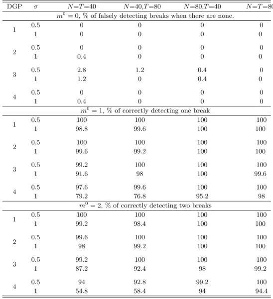
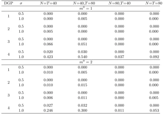
We first evaluate the probability of falsely detecting breaks when there is no break in the simulation design. Then we experiment on the DGPs with one or two breaks. We evaluate the probability of correctly detecting the number of breaks and the accuracy of break date estimation when breaks are detected. Tables 1, 2 and 3 report simulation results for the above DGPs. The first panel of Table 1 reports the percentages of falsely detecting breaks when there is no break (m0 = 0). The second and the third panels report the percentages of correctly estimating the number of breaks when the true number of breaks is one and two, respectively. In Table 2, we report the ratio of average Hausdorff distance (HD) between the estimated and true sets of breaks to T, i.e., 100·HD(Tbmb,Tm00)/T, conditional on correct estimation of the number of breaks. Here the average is taken over 250 replications and the HD between two sets A and
B is defined as HD(A, B) = max{D(A, B), D(B, A)} with D(A, B) ≡ supb∈Binfa∈A|a−b|.
The mean squared or absolute errors of the parameter estimates are roughly proportional to the Hausdorff error of the break-date estimation and hence are not reported. In Table 3 we report
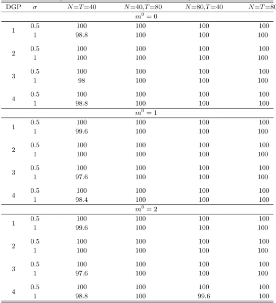
the percentages of correctly estimating the number of factors in the Monte Carlo replications. We summarize the major findings from these tables. (i) When there is no break in the DGPs, the probabilities of falsely detecting breaks decline to zero as either N or T increases. (ii) When there are one or two breaks, the probabilities of correctly estimating the number of breaks converge fairly quickly to 100% or near 100% as both N and T increase. The detection procedure performs slightly better at lower idiosyncratic noise levels (σ = 0.5) than at higher noise level (σ = 1). The performance is robust to serial correlation in the common factor, serial correlation and conditional heteroskedasticity in the errors, and the dependence of both the factors and their loadings on the regressor. For the dynamic panel (DGP-4), the procedure performs less satisfactorily. However, this may be due to the fact that the signal-to-noise ratio in this case is roughly 1/3, much less than that in the other three DGPs. (iii) Conditional on the correct estimation of the number of breaks, our procedure estimates the break dates accurately, which can be seen from Table 2 (iv) Finally, Table 3 shows that the BIC-type information criterion specified in (4.1) can accurately determine the number of factors for the interactive fixed effects structure.
5
An empirical application to the environmental Kuznets curve
The environmental Kuznets curve (EKC) has become a standard feature in the environmental policy literature. It hypothesizes that the relationship between income and the emission of chemicals like sulfur dioxide (SO2) and carbon dioxide (CO2) or the natural resource usage has
an inverted U-shape, which is similar to the relationship between income and inequality in the Kuznets curve hypothesis in economics. In this section we consider the following specification:
cit=β0t+β1tyit+β2ty2it+β3teit+λ′ift+uit,
wherecitrepresents the logarithm of per capita CO2emission for countryiin yeart,yitrepresents
the logarithm of per capita income (gross domestic product, abbreviated as GDP),eitrepresents
the logarithm of per capita consumption of energy,ftis a vector of unobservable common factors
andλi is a vector of factor loadings. Our data-driven BIC criterion determines that the number
of factors is five. The controlling of energy consumption in EKC studies was used in the time series regression setting in Ang (2007), and the panel data setting in Apergis and Payne (2009, 2010), Lean and Smyth (2010), Arouri et al. (2012) and Farhani et al. (2014). The panel data
Table 1: The probabilities for falsely detecting breaks when there are none and of correctly detecting the breaks when there are breaks
DGP σ N=T=40 N=40,T=80 N=80,T=40 N=T=80
m0
= 0, % of falsely detecting breaks when there are none.
0.5 0 0 0 0 1 1 0 0 0 0 0.5 0 0 0 0 2 1 0.4 0 0 0 0.5 2.8 1.2 0.4 0 3 1 1.2 0 0.4 0 0.5 0 0 0 0 4 1 0.4 0 0 0 m0
= 1, % of correctly detecting one break
0.5 100 100 100 100 1 1 98.8 99.6 100 100 0.5 100 100 100 100 2 1 99.6 99.2 100 100 0.5 99.2 100 100 100 3 1 91.6 98 100 99.6 0.5 97.6 99.6 100 100 4 1 79.2 76.8 95.2 98 m0
= 2, % of correctly detecting two breaks
0.5 100 100 100 100 1 1 99.2 98.4 100 100 0.5 99.6 100 100 100 2 1 98 99.2 100 100 0.5 99.2 100 100 100 3 1 87.2 92.4 98 99.2 0.5 94 92.8 99.2 100 4 1 54.8 58.4 94 94.4
Table 2: Estimation accuracy for the break dates when there is one or two structural breaks DGP σ N=T=40 N=40,T=80 N=80,T=40 N=T=80 m0 = 1 0.5 0.000 0.000 0.000 0.000 1 1.0 0.000 0.005 0.000 0.000 0.5 0.000 0.000 0.000 0.000 2 1.0 0.005 0.000 0.000 0.000 0.5 0.000 0.000 0.000 0.000 3 1.0 0.066 0.051 0.000 0.000 0.5 0.020 0.030 0.000 0.000 4 1.0 0.423 0.540 0.037 0.092 m0= 2 0.5 0.000 0.000 0.000 0.000 1 1.0 0.010 0.005 0.000 0.000 0.5 0.000 0.000 0.000 0.000 2 1.0 0.010 0.015 0.000 0.000 0.5 0.000 0.000 0.000 0.000 3 1.0 0.006 0.011 0.000 0.005 0.5 0.027 0.032 0.000 0.000 4 1.0 0.246 0.300 0.011 0.053
Note. The table reports 100·HD(Tbmb,T0
m0)/T,averaged over 250 replications.
studies in the existing literature, however, assume that the coefficients are constant over time. In our specification, we not only introduce the interactive fixed effects in the panel data models but also allow time-varying coefficients that may capture the instability of the EKC brought by the changing social, political, and economic environment in the past few decades.
We obtain the panel data set from World Bank Development Indicators. The CO2emission is
measured in metric tones per capita, income is measured using per capita real GDP in constant 2000 USD, and energy consumption is measured with kilogram of oil equivalent per capita. The time frame is selected to be 1971-2010. We exclude OPEC countries, small countries whose populations are less than six million, and other countries with missing observations during the time span. In total, we have N = 74 countries and T = 40 time points.
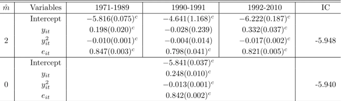
The results are summarized in Table 4. The information criterion defined in (4.2) selects a tuning parameter that identifies two breaks ( ˆm = 2) in 1990 and 1992. In the first regime of 1971-1990, the EKC hypothesis is confirmed, as the coefficient on the squared income is significantly negative, implying an inverted U-shape. The elasticities of CO2emission per capita
Table 3: The probabilities for correctly estimating the number of factors DGP σ N=T=40 N=40,T=80 N=80,T=40 N=T=80 m0 = 0 0.5 100 100 100 100 1 1 98.8 100 100 100 0.5 100 100 100 100 2 1 100 100 100 100 0.5 100 100 100 100 3 1 98 100 100 100 0.5 100 100 100 100 4 1 98.8 100 100 100 m0 = 1 0.5 100 100 100 100 1 1 99.6 100 100 100 0.5 100 100 100 100 2 1 100 100 100 100 0.5 100 100 100 100 3 1 97.6 100 100 100 0.5 100 100 100 100 4 1 98.4 100 100 100 m0= 2 0.5 100 100 100 100 1 1 99.6 100 100 100 0.5 100 100 100 100 2 1 100 100 100 100 0.5 100 100 100 100 3 1 97.6 100 100 100 0.5 100 100 100 100 4 1 98.8 100 99.6 100
Table 4: A panel data estimation of the EKC for 74 countries from 1971 to 2010 ˆ m Variables 1971-1989 1990-1991 1992-2010 IC Intercept −5.816(0.075)c −4.641(1.168)c −6.222(0.187)c yit 0.198(0.020)c −0.028(0.239) 0.332(0.037)c 2 y2 it −0.010(0.001)c −0.004(0.014) −0.017(0.002)c -5.948 eit 0.847(0.003)c 0.798(0.041)c 0.821(0.005)c Intercept −5.841(0.037)c yit 0.248(0.010)c 0 y2 it −0.013(0.001)c -5.940 eit 0.842(0.002)c
Note. Superscripta, bandcdenotes significance level at 10%, 5%, and 1%, respectively. Standard errors are given in parentheses.
logarithm of real GDP per capita. The threshold, or the turning points of the EKC, occurs at the per capita income of 19,900 USD (2000). The second regime is a short one, covering only two years, 1990 and 1991. In this regime, the coefficients on both yit and yit2 are statistically
insignificant. The signs of these coefficients do not point to an inverted U-shape. This suggests that, using a short panel or cross-section data set collected in a certain time period, one may reject the EKC hypothesis, while a longer panel data would arrive at the opposite conclusion. In the third regime of 1992-2010, the EKC hypothesis is again confirmed. The elasticities of CO2emission per capita with respect to real income per capita in the regime is (0.332−0.034y),
implying a threshold of 17,400 USD (2000). Comparing with the first regime, we may conclude that the EKC has shifted leftward in the past two decades. The second regime of 1990-1991 may be regarded as a transition period from the first regime to the second regime, which is more environment-friendly. We also report in Table 4 the case of zero break ( ˆm = 0), where coefficients are assumed to be constant. Here the EKC hypothesis is also confirmed, with a threshold at 13,900 USD (2000). Interestingly, the panel data model with constant regression coefficients paints the most optimistic EKC. If we estimate the regression coefficients in the panel data model with two structural breaks detected by the PPC method, however, we see a more cautious picture for the EKC.
6
Conclusions
In this paper, we study the estimation of the panel data models with interactive fixed effects and multiple structural breaks, which substantially generalizes the existing work which either
considers the panel models with interactive fixed effects but no structural break (c.f., Bai, 2009), or the panel models with multiple structural breaks but under cross-sectional independence (c.f., Qian and Su, 2015b). We develop a novel PPC estimation procedure with the AGF-LASSO penalty function to consistently estimate both the regression coefficients and the factor loadings. Under some regularity conditions, we show that both the unknown number of structural breaks and the unobservable break dates can be consistently estimated. In order to further improve the convergence rates, we also estimate the regression coefficients (in different regimes) through the post-LASSO method and then establish the asymptotic distribution theory of the resulting estimators. In particular, the developed shrinkage estimation methodology and the asymptotic theory are also applicable to the case of dynamic panel data. We introduce two data-driven methods to determine the number of factors and choose the tuning parameter involved in the PPC estimation procedure, respectively. The simulation studies show that the proposed PPC method has a high probability of correctly estimating the number of breaks when the structural breaks exist in the simulation design, and a low probability of false detection when there is no structural break. We apply our method to study the EKC for 74 countries over 40 years and find two breaks in the panel data.
Appendix
We first give in Appendix A some regularity conditions that are used to derive the asymptotic results. Then we provide some technical lemmas and prove the main theoretical results in Appendix B. The proofs of the technical lemmas are given in Appendix C of the supplemental document.
A
Assumptions
We start with the introduction of some notation. Denote
δN T = min( √ N ,√T), δp,N T = min( p N/p,√T), ∆N T = min 1≤j≤m0 α0j+1−α0j, ∆∗N T = max 1≤j≤m0 α0j+1−α0j.
Letξij =PTt=1εitεjt for 1≤i, j≤N, and ξ∗ts =PNi=1εitεis for 1≤t, s≤T. Define
ΩN T =ΦN T −Φ∗N T, ΦN T =diag Φ1, ...,Φm0+1
where Φj = 1 N τj(T) T0 j−1 X t=T0 j−1 Xt′MΛ0Xt, Φ∗jk = 1 N T τj(T) T0 j−1 X t=T0 j−1 T0 k−1 X s=T0 k−1 χstXt′MΛ0Xs, τj(T) =Tj0−Tj0−1 and χst =fs0′ T1F 0′F0+
ft0. In order to prove the asymptotic results stated in Sections 3 and 4, we make the following assumptions.
Assumption 1 (i) There exist two positive definite matricesΣF and ΣΛ such that
1 TF 0′F0 P →ΣF, 1 NΛ 0′Λ0 P →ΣΛ.
Furthermore, both the common factorsf0
t and the factor loadingsλ0i have finite 8-th moments.
(ii) Let the regressorXt satisfy max1≤t≤T kXtk=OP p1/2N1/2, and
cx≤inf Λ 1min≤t≤Tµmin N −1X′ tMΛXt≤ max 1≤t≤Tµmax N −1X′ tXt≤c∗x
w.p.a.1, where 0< cx < c∗x <∞, and infΛ is taken with respect to Λsuch that N1Λ
′Λ=I
R0.
(iii) Let ε= (ε1, ..., εT). The idiosyncratic error termεit satisfiesE[εit] = 0 and E[ε8it]< cε for
each iand tand kεksp=max(√N,√T).wherecε is a bounded positive constant. Furthermore,
max 1≤s,t≤TE kX′ tεsk2=O(pN), max 1≤t≤TE kΛ0′εtk2=O(N), EkΛ0′εF0k2=O(N T), max 1≤i,j≤NE hXT t=1 T X s=1 εitεjsγtγ′s 2i =O(T2 ), and max 1≤i,j≤NE hXT t=1 T X s=1 εitεjsε′tεs 2i =O(N2 T2 +T4 ),
where γt can be either 1 orf0
t.
(iv) Assume that max1≤i,j≤NVar(ξij) = max1≤i,j≤NVar(PTt=1εitεjt) =O(T), and there exists σij >0 such that E(ξij)≤σijT and PNi=1 PN j=1σ2ij =O(N). Furthermore, we have max 1≤t≤TE hXT s=1 (ξ∗ts)2i=O N2+N T, Eh T X t=1 T X s=1 ft0′ξ∗tsfs02i=O N2T2.
Assumption 2 (i) The tuning parameterγ satisfies that
γ =o(1), γm0∆N T−κδp,N T =O(1) as (N, T)→ ∞,
whereκ is the user-specified positive constant defined in (2.3).
(ii) Let the following restrictions hold:
(iii) Let γδκp,N T+1 → ∞ as (N, T)→ ∞.
Assumption 3 (i) There exists a positive definite matrixΩ0 such thatΩN T −Ω0sp =oP(1).
(ii) There exist 0< cτ ≤c∗τ <∞ such that
cτT
m0 ≤1≤jmin≤m0+1τj(T)≤1≤jmax≤m0+1τj(T)≤
c∗τT m0.
(iii) Letting At=PTs=1Λ0′εsε′sεt, max1≤t≤TE(A2t) =O(N2(N+T)).
(iv) Letting Wj,N T = N τ1j(T)P T0 j−1 t=T0 j−1 X′ tMΛ0(εt −εt∗) for j = 1, ..., m0 + 1 and WN T = (W′
1,N T, ..., Wm′ 0+1,N T)′,there exist BN T(3) andΩ1 such that
S∗DN T[WN T −BN T(3)]−→D N 0, S∗Ω1S′∗
,
whereDN T is defined in Section 3.2,S∗ is an arbitraryk0×p(m0+ 1) matrix with full row rank, and k0 is a fixed positive integer.
(v) Let (N T)1/2/δ3p,N T =o(1) andp/δp,N T =o(1) as (N, T)→ ∞.
Assumption 4 As (N, T)→ ∞, ρ1 →0 andδ2p,N Tρ1→ ∞.
Assumption 5 (i) For any 0≤m < m0, there exists a positive constant cβ such that
min Tm min αm m0 T∆2 N T mX+1 j=1 TXj−1 t=Tj−1 β0t−αj 2 ≥cβ,
whereαm and Tm are defined in Section 3.2.
(ii) As (N, T)→ ∞, T∆m20 N T(pN
−1/2+p1/2T−1/2) =o(1).
(iii) As (N, T)→ ∞, m0pρ
2→0 and δ2p,N Tpρ2 → ∞.
Remark A.1. Assumption 1 imposes some standard moment conditions on Xit, ft0, λ0i and
εit, which are analogous to those in the existing literature such as Bai and Ng (2002), Bai
(2009), Bai and Li (2014), Lu and Su (2015), and Moon and Weidner (2015). As we allow p, the dimension of the regression coefficients, to be divergent, some of our moment conditions might be slightly stronger than those in the literature. Assumptions 1(iii) and (iv) allow weak form of cross-sectional dependence and serial dependence among Xit,ft0,λ0i and εit.In
partic-ular, unlike Pesaran (2006) and Bai (2009), we do not assume independence between εit and
(Xjs, fs0, λ0j) for all i, j, t, s, and our theories are thus applicable to the dynamic autoregressive
panel data models with interactive fixed effects. Assumption 2 imposes some mild restrictions on the tuning parameterγ and the jump sizes of the regression coefficients, which can be easily
justified. For example, assuming that the jump sizes are bounded away from zero and infinity and N ∼ T, Assumption 2 can be simplified to γ = o(1), γm0(N/p)1/2 = O(1), p = o(N1/2) and γ(N/p)(κ+1)/2 → ∞. Assumption 3 imposes some additional conditions for the proof of
the asymptotic distribution theory of the post-LASSO estimation, which can be verified under some primitive conditions. For example, if we assume that {εit, λ0i} are independent across i
and for eachi,{εit}is a martingale difference sequence with respect to theσ-field generated by
(εi,t−1, . . . , εi1, ft0−1, . . . , f10, λ0i) and {εit, Xit} satisfy some strongly mixing conditions, then the
moment condition in Assumption 3(iii) holds. Assumption 4 indicates that ρ1 has to shrink to zero at an appropriate rate to avoid both over-selection and under-selection of the number of factors. Assumptions 5(i)(ii) impose conditions to avoid the selection of model with fewer breaks than the true number by using an information criterion proposed in Section 4.2. Assumption 5(iii) parallels Assumption 4.
B
Proofs of the main asymptotic results
In this appendix, we give the detailed proofs of the asymptotic results in Sections 3 and 4. We start with two technical lemmas whose proofs are provided in Appendix C of the supplemental document.
Lemma B.1 Suppose that Assumption 1 in Appendix A holds and pN−1/2+p1/2T−1/2=o(1).
Let β˙ = β˙′ 1, ...,β˙′T
′
be the preliminary estimates of the regression coefficients which mini-mize, QˆN T(β,Λ), the first term of the objective function defined in (2.4). Then
β˙ t−β0t = OP p1/2N−1/2+T−1/2 = OP
δ−p,N T1 for any t = 1,2, ..., T, where δp,N T is defined as in
Appendix A.
Lemma B.2 Suppose that Assumption 1 Appendix A holds and let ηN T = T1 PTt=1kβˆt−β0tk2. Then we have (i) N T1 PTt=1(ˆβt−β0t)′X′ tMΛˆεt=OP δ−p,N T1 η1N T/2, (ii) PTt=1f0′ t Λ0′MΛˆεt=OP δ−N T2 +δ−p,N T1 η1N T/2, and (iii) N T1 PTt=1ε′ t PΛˆ −PΛ0εt=OP δ−2 N T .
We next give the proof of Theorem 3.1 by using the above two lemmas.
Proof of Theorem 3.1. (i) Recall that the penalized estimate of β0 is denoted by ˆβ = ˆ
β′1, ...,βˆ′T′ and the estimated factor loading matrix is denoted by ˆΛ. Note that
Then, by (B.1) and using the fact thatMΛ0Λ0 =0, we have ˆ QN T,γ βˆ,Λˆ−QˆN T,γ β0,Λ0 = 1 T T X t=1 h ˆ Q∗N T,t(βt,Λ) + ˆQ⋄N T,t(βt,Λ)i +γ T X t∈T0 m0 ˙ wthβˆt−βˆt−1 −β0t−β0t−1 i +γ T X t∈Tc ˙ wt hˆ βt−βˆt−1−β0t −β0t−1i, (B.2) where ˆ Q∗N T,t(βt,Λ) = 1 N h ˆ βt−β 0 t ′ Xt′MΛˆXt βˆt−β 0 t −2 ˆβt−β 0 t ′ Xt′MΛˆΛ 0 f0 t +f 0′ t Λ 0′ MΛˆΛ 0 f0 t i , ˆ Q⋄N T,t(βt,Λ) = 1 N h −2 ˆβt−β 0 t ′ Xt′MΛˆεt+ 2ft0′Λ 0′ MΛˆεt−ε′tPΛˆεt+ε′tPΛ0εt i .
As β0t−β0t−1 =0 fort∈ Tc, the last term on the right hand side of (B.2) satisfies that
γ T X t∈Tc ˙ wthβˆt−βˆt−1 −β0t−β0t−1 i= γ T X t∈Tc ˙ wtβˆt−βˆt−1 ≥0. (B.3)
By the triangle inequality, the Cauchy-Schwarz inequality, Lemma B.1 and Assumption 2(ii) in Appendix A, we can prove that
X t∈T0 m0 ˙ wt hˆ βt−βˆt−1−β0t −β0t−1i ≤ OP(∆−N Tκ) X t∈T0 m0 βˆ t−β0t ≤ OP(∆−N Tκ)(m0)1/2 X t∈T0 m0 βˆ t−β0t 2 1/2 ≤ OP(∆−N Tκ)(m0T)1/2 1 T T X t=1 βˆ t−β0t 2 !1/2 .
Note that Assumption 2(i) implies thatγ(m0)1/2T−1/2∆−κ N T =o(δ
−1
p,N T) whereδp,N T = min(
p
N/p,√T). This, together with the above argument, indicates that
γ T X t∈T0 m0 ˙ wt hˆ βt−βˆt−1−β0t −β0t−1i=oP δ−p,N T1 η1N T/2. (B.4)
By Lemma B.2, we can readily show that 1 T T X t=1 ˆ Q⋄N T,t(βt,Λ) =OP δ−N T2 +δp,N T−1 η1N T/2. (B.5)
Combining (B.4) and (B.5), we have ˆ QN T,γ βˆ,Λˆ−QˆN T,γ β0,Λ0≥ 1 T T X t=1 ˆ Q∗N T,t(βt,Λ) +OP δ−N T2 +δp,N T−1 η1N T/2. (B.6) Define the vectors:
ˆ
dβ = ˆβ−β0 and ˆdΛ =
1
N1/2vec(MΛˆΛ 0),
wherevec(·) denotes the vectorization of a matrix; and define the matrices: ˆ A = 1 Ndiag X ′ 1MΛˆX1, ..., XT′ MΛˆXT, Bˆ = (F0′F0)⊗IN, and ˆ C = 1 N1/2 f10⊗MΛˆX1, ..., fT0 ⊗MΛˆXT,
where⊗ denotes the Kronecker product. It is easy to verify that 1 N T T X t=1 ˆ βt−β0t′Xt′MΛˆXt βˆt−β0t = 1 Tˆd ′ βAˆdˆβ, 1 N T T X t=1 ˆ βt−β0t′Xt′MΛˆΛ0ft0= 1 N T T X t=1 TrnMΛˆΛ0ft0 βˆt−β0t ′ Xt′MΛˆ o = 1 Tdˆ ′ ΛCˆdˆβ, 1 N T T X t=1 ft0′Λ0′MΛˆΛ0ft0 = 1 N T T X t=1 TrMΛˆΛ0ft0ft0′Λ0′MΛˆ = 1 Tdˆ ′ ΛBˆdˆΛ,
where we have used the following facts on matrix calculation: Tr A1A2A3 =vec′ A1 A2 ⊗
Ikvec A3 and Tr A1A2A3A4 = vec′ A1 A2 ⊗A′4
vec A′3 with k being the size of the column vectors in A3. Using the above notations, we may show that
1 T T X t=1 ˆ Q∗N T,t(βt,Λ) = 1 T dˆ ′ βAˆdˆβ−2ˆd ′ ΛCˆdˆβ+ ˆd ′ ΛBˆdˆΛ= 1 T dˆ ′ βDˆdˆβ+ ˆd ′ ∗Bˆdˆ∗ , (B.7) where ˆD= ˆA−Cˆ′Bˆ+Cˆ and ˆd∗= ˆdΛ−Bˆ +ˆ
Cdˆβ. By Assumption 1(i), we may show that the min-imum eigenvalue of T1Bˆ is bounded away from zero w.p.a.1, i.e., there exists a positive constant
c1such thatµmin Bˆ/T
> c1for sufficiently largeT. We next show thatµmax Cˆ ′ˆ
C/T=oP(1).
Lettingνst=fs0′ft0, it is easy to verify that
ˆ C′Cˆ = 1 N ν11X1′MΛˆX1 ν12X1′MΛˆX2 ... ν1TX1′MΛˆXT ν21X2′MΛˆX1 ν22X2′MΛˆX2 ... ν2TX2′MΛˆXT .. . ... . .. ... νT1XT′MΛˆX1 νT2XT′MΛˆX2 ... νT TXT′ MΛˆXT .
Letting ˆ C1 = 1 N ν11X1′MΛˆX1 ν12X1′MΛˆX2 ... ν1TX1′MΛˆXT 0 ν22X2′MΛˆX2 ... ν2TX2′MΛˆXT .. . ... . .. ... 0 0 ... νT TXT′MΛˆXT
and ˆCd= N1diag ν11X1′MΛˆX1, ..., νT TXT′ MΛˆXT, we have
ˆ
C′Cˆ = ˆC1+ ˆC ′
1−Cˆd. (B.8)
By the fact that the eigenvalues of a block upper/lower triangular matrix are the combined eigenvalues of its diagonal block matrices, Weyl’s inequality, and Assumptions 1(i) and (ii), we have
T−1µmax( ˆC′Cˆ) ≤ T−1{2µmax( ˆC1)−µmin( ˆCd)}
≤ 2T−1 max
1≤t≤T
ft02µmax N−1Xt′MΛˆXt
= OP(T−1)OP(T1/4)OP(1) =OP(T−3/4),
where we use the fact that max1≤t≤Tkft0k2 =OP T1/4 by Assumption 1(i) and the Markov
inequality. On the other hand, we note that the minimum eigenvalue of ˆA is positive and bounded away from zero w.p.a.1. Hence, the matrix ˆD is asymptotically positive definite as its minimum eigenvalue is positive and bounded away from zero w.p.a.1 by using the above facts. Then, by (B.7) and (B.8), we can readily show that there exist two positive constantsc2 andc3
such that c2 Tkdˆβk 2+c 3kdˆ∗k2≤ 1 T T X t=1 ˆ Q∗N T,t(βt,Λ), (B.9)
which indicates that
c2 Tkdˆβk 2+c 3kˆd∗k2+OP δ−N T2 +δ−p,N T1 η 1/2 N T ≤QˆN T βˆ,Λˆ−QˆN T β0,Λ0. (B.10)
Multiplying both sides of (B.10) by δ2p,N T and noting that T1kˆdβk2 = ηN T and ˆQN T βˆ,Λˆ−
ˆ
QN T β0,Λ0≤0, we readily show that
c2δ2p,N TηN T +OP(1) +OP(1)·δ2p,N TηN T
1/2
≤0. (B.11)
Whenδ2p,N TηN T is sufficiently large, the first term on the left hand side of (B.11) would dominate the other two terms, which would lead to a contradiction. Hence, we must have thatδ2p,N TηN T
is stochastically bounded, implying thatηN T =OP pN−1+T−1.This completes the proof of
Theorem 3.1(i).
(ii)The proof for the point-wise convergence result is similar to the proof of Theorem 3.2(ii) in Qian and Su (2015b), where the condition γm0∆−κ
N Tδp,N T =O(1) in Assumption 2(i) is used
to handle the penalty term. We omit the details to save space.
We have thus completed the proof of Theorem 3.1.
Proof of Theorem 3.2. To prove the sparsity, it is equivalent to showing P ˆθt
6= 0 for some t∈ Tc→0 (B.12) as (N, T)→ ∞. We consider two cases: (i) 2≤t≤T−1 and t∈ Tc; and (ii)t=T and t∈ Tc. Recall that δp,N T = min(p−1/2N1/2, T1/2).
For case (i), there would be two possible circumstances: (i.1) t+ 1 = T0
j ∈ Tm00 for some
j = 1, ..., m0; and (i.2) t+ 1 ∈ Tc. We invoke subdifferential calculus (e.g., Bersekas, 1995, Appendix B.5) to obtain the following Karush-Kuhn-Tucker condition with respect toβt to the objective function in (2.4): δp,N T " −2 N X ′ tMΛˆ Yt−Xtβˆt +γw˙t ˆ βt−βˆt−1 βˆ t−βˆt−1 −γw˙t+1 ˆ βt+1−βˆt βˆ t+1−βˆt # =0, (B.13) where for any p×1 vector a with kak = 0, a/kak is defined as an arbitrary p ×1 vector with Frobenius norm smaller than or equal to 1. Let UN T,1 = N1Xt′MΛˆ Yt−Xtβˆt
, UN T,2 = γw˙t ˆ βt−βˆt−1 βˆ t−βˆt−1 and UN T,3 = γw˙t+1 ˆ βt+1−βˆt βˆ t+1−βˆt
. Following the proof of Theorem 3.1 and using
Lemma B.2, we may show that
δp,N TkUN T,1k=OP(1). (B.14)
If circumstance (i.1) holds, by Lemma B.1 and Assumption 2(ii), we have ˙ wt+1=kβ˙t+1−β˙tk−κ ≤ h min 1≤j≤m0 α0j+1−α0j+OP δ−p,N T1 i −κ =OP(∆−N Tκ), (B.15)
which together with Assumption 2(i), indicates that
δp,N TkUN T,3k=OP(γδp,N T∆−N Tκ) =OP(1). (B.16)
However, for case (i) with 2≤t≤T −1 andt∈ Tc, by Lemma B.1, we may show that w.p.a.1 ˙
for some positive constant C. Hence, it is not difficult to see that when ˆθt6=0,
δp,N TkUN T,2k ≥Cγδκp,N T+1 → ∞ (B.18)
by using Assumption 2(iii). By (B.14), (B.16) and (B.18), the equation (B.13) cannot hold as (N, T) → ∞. Hence, ˆθt can only take the value of 0 at which ||ˆθt|| is not differentiable.
Furthermore, as an implication of the above result, if t= T0
j −1 ∈ Tc for some j = 1, ..., m0, then we have δp,N Tγw˙t ˆ βt−βˆt−1 βˆ t−βˆt−1 =δp,N Tγw˙T0 j−1 ˆ βT0 j−1− ˆ βT0 j−2 βˆ T0 j−1− ˆ βT0 j−2 =OP(1). (B.19)
We next prove (B.12) for circumstance (i.2). Following the above argument, we can show that whent=Tj0−2 and ˆθT0
j−26=0, δp,N T N X ′ tMΛˆ Yt−Xtβˆt =OP(1), δp,N Tγw˙t ˆ βt−βˆt−1 βˆ t−βˆt−1 → ∞, (B.20)
which, together with (B.19), implies that (B.13) cannot hold as (N, T)→ ∞. Hence, ˆθT0 j−2 can
only be 0. Deducting in this way until we reach t=T0
j−1+ 1∈ Tc, we can complete the proof
of sparsity for case (i).
For case (ii), note that the consequence of the Karush-Kuhn-Tucker condition with respect toβT leads to δp,N T " 1 NX ′ TMΛˆ YT −XTβˆT +γw˙T ˆ βT −βˆT−1 βˆ T −βˆT−1 # =0. (B.21)
As there is only one penalty term in (B.21), the proof is much simpler than that for case (i). Hence, we omit the details here.
We have completed the proof of Theorem 3.2.
Proof of Corollary 3.3. By Theorem 3.2, as (N, T)→ ∞, no time point inTccan be identified as the break time, which implies that ˆm ≤ m0. On the other hand, by Theorem 3.1, for any
t∈ Tm00, ˆθt =βˆt−βˆt−1=βt0−β0t−1+OP(δ−p,N T1 ) =θ0t +OP(δ−p,N T1 ),
which indicates thatkθ0tk=OP(δp,N T−1 ) if ˆθt=0 (i.e.,t∈ Tm00 is not identified as a break point). However, the conclusionkθ0tk=OP δ−p,N T1
is assumed in Assumption 2(ii). Hence, each time point in Tm00 must be identified as the break time, which implies that ˆm=m0 w.p.a.1 and thus both the results (i) and (ii) are proved. To prove the asymptotic distribution theory for the post-LASSO estimator in Theorem 3.4, we need to use the following lemma whose proof is given in Appendix C of the supplemental document. Let ˜Λm0 ≡ Λ˜(T0
m0) be the infeasible estimator of the factor loadings in the post-LASSO estimation procedure, ˜H = T1F0′F0 N1Λ0′ Λ˜m0
˜
V+N T, and ˜αm0 ≡α˜m0(T0
m0), where ˜
VN T will be defined later in (B.25).
Lemma B.3 Suppose that the conditions in Theorem 3.4 hold. Then, (i) for each j= 1, ..., m0+ 1, we have
N τ1 j(T) T0 j−1 X t=T0 j−1 Xt′ MΛ˜ m0−MΛ0 εt+BN T,j(2,1) =OP δ−N T1 (m0)−1/2kα˜m0 −α 0k+δ−3 p,N T ,
where τj(T) and BN T,j(2,1) are defined as in Theorem 3.4;
(ii) for each j= 1, ..., m0+ 1, we have
N τ1 j(T) T0 j−1 X t=T0 j−1 Xt′MΛ˜ m0 Λ 0−Λ˜ m0H˜ + ft0+ 1 N τj(T) T0 j−1 X t=T0 j−1 Xt′MΛ0ε∗t +BN T,j(1) −BN T,j(2,2) + Φ∗j1, ...,Φ∗j,m0+1 ( ˜αm0 −α0) =OP pδ−p,N T1 (m0)−1/2kα˜m0−α 0k+δ−3 p,N T ,
where ε∗t = T1 PTs=1χstεs, Φ∗jk, 1≤ j, k≤m0+ 1, are defined at the beginning of Appendix A,
and BN T,j(1) and BN T,j(2,2), j = 1, ..., m0+ 1, are defined as in Theorem 3.4.
We are now ready to prove Theorem 3.4.
Proof of Theorem 3.4. Let GT =Tˆj =Tj0 forj = 1, ..., m0 . By Corollary 3.3, we readily
have PnSDN T α˜mˆ −α0)∈ C mˆ =m0o = PnSDN T α˜mˆ −α0)∈ C,GT mˆ =m0o+PnSDN T α˜mˆ −α0)∈ C,GTc mˆ =m0o = PnSDN T α˜m0 −α0)∈ C o +o(1), (B.22) where C ⊂ Rk0, Gc
T is the complement of GT and ˜αm0 = ˜αm0(Tm0) is the infeasible estimate of α0. Hence, throughout the proof, we can replace ˆm and ˆTj (j = 1, ...,mˆ) by m0 and Tj0,