Techniques for model construction
in separation logic
Jonas B. Jensen September 2013Contents
1 Introduction 2 1.1 Overview . . . 21.2 What is a separation logic? . . . 3
1.3 Contributions . . . 3
2 Semantics of the programming language 4 2.1 Modelling failure . . . 6 2.2 Modelling concurrency . . . 7 3 Assertion logic 8 3.1 Heyting algebras . . . 8 3.2 BI algebras . . . 13 3.3 Separation algebras . . . 16 3.4 Program variables . . . 25 4 Specifications 33 4.1 Hoare triples . . . 33 4.2 Specification logic . . . 37 4.3 Alternative formulations . . . 41 5 Conclusion 43 Index 45
1
Introduction
Separation logic has been very successful at giving concise specifications and short proofs to pointer-manipulating programs. Unfortunately, the term
separation logic covers a whole zoo of different theories. Almost every pub-lication that applies separation logic starts by defining a new logic that is general enough to attack the problem at hand but not so general that it disturbs the presentation with orthogonal features.
This proliferation of theories has been identified as a problem several times [BBTS05, Par10], but that has not stopped the flow of new logics being created. Given that no logic proposed so far is a generalisation of all others, we should welcome more exploration and diversity for the foreseeable future.
For new researchers in the field, the best sources for building an intu-itive as well as formal understanding of separation logic are still the original articles from 2001-2002 [Rey02, IO01]. Unfortunately, this leads many re-searchers to ignore some of the recent advances that lead to more general theories with simpler and more concise presentation and metatheory.
This chapter attempts to summarise those advances in the hope that it will allow new research on separation logic to start from the cutting edge as of 2013 instead of 2002. The reader is assumed to have some familiarity with separation logic. A good place to start would be the 2002 introduction by Reynolds [Rey02] or the 2012 tutorial by O’Hearn [O’H12]. More in-depth theoretical discussions are found in [IO01] and [Rey11], although these are still introductory texts.
The level of formal detail in this chapter will be quite high since it aims to be useful for readers trying to encode separation logic in a proof assistant or building a stand-alone tool.
1.1 Overview
The general recipe for making a separation logic, and the structure of this chapter, is as follows.
1. Choose aprogramming language. Small variations in the definition and semantics of the language can have great consequences for the ease of building a separation logic for it.
2. Design theassertion logic; i.e., the formulas that describe machine state. It typically includes separating conjunction and points-to formu-las. Assertion-logic formulas are typically modelled as sets of machine state subject to some instrumentation and/or side conditions.
3. Design the specification logic; i.e., the formulas that describe com-putations. It typically includes Hoare triples, which refer to assertions
in their pre- and postconditions. In some higher-order settings, the assertion logic may also refer to specifications, in which case the defi-nitions of these two logics may have to be mutually recursive or may coincide.
There is also an optional 0’th step: choose a metalogic; i.e., a math-ematical framework in which to formulate the theory. The metalogic is usually implicitly chosen as “standard math as taught in school”, but re-cent examples have shown that some separation logics become both sim-pler and more general when embedded in a metalogic that provides, for example, bound names [Pit01], dependent types [KBJD13] or step-indexing [SB13a, BMSS12].
1.2 What is a separation logic?
To limit the scope of this text, we impose some minimum requirements on what is considered a separation logic. We will say it must contain:
1. An logic of assertions P, Q, R that is a complete BI algebra; i.e., it satisfies the rules in Figure 2 (page 9) and Figure 4 (page 13).
2. A logic of specifications S that is a complete Heyting algebra; i.e., it satisfies the rules in Figure 2.
3. A Hoare-triplespecification of the form {P}c{Q} or a generalisa-tion thereof. The Hoare triple must satisfy
P `P0 S ` {P0}c{Q0} Q0 `Q Consequence S ` {P}c{Q} S ` ∀x.{P(x)}c{Q} Exists S ` {∃x. P(x)}c{Q} S` {P}c{Q} Frame S` {P ∗R}c{Q∗R}
These requirements are somewhat imprecise, but they have to be, since they apply to logics that have yet to be invented.
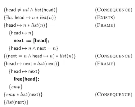
The inference rules required of the triple ensure that it admits the narra-tion style of writing a Hoare-logic proof [Rey11, WDP13], where commands are interleaved with assertions. Figure 1 shows an example proof narration that uses all three rules.
1.3 Contributions
The main contribution of this chapter is to survey a portion of the first twelve years of separation-logic literature in a common mathematical framework. There is too much published literature to mention it all, so the focus is on techniques that are needed everywhere rather than the very latest develop-ments in specific areas such as concurrency.
{head6=nil∧list(head)} (Consequence) {∃n.head7→n∗list(n)} (Exists)
{head7→n∗list(n)} (Frame) {head7→n}
next := [head]; {head7→n∧next=n}
{(next=n∧head7→n)∗list(n)} (Consequence) {head7→next∗list(next)} (Frame)
{head7→next} free(head); {emp}
{emp∗list(next)} (Consequence) {list(next)}
Figure 1: Narration-style proof of a two-line example program.
The chapter follows the same structure as any other article that defines a programming language and builds a separation logic for it, but along the way we discuss alternatives and variations at every point. A particularly thorough treatment is given to separation algebras, since their theory is highly scattered across the literature and often stated in a much less general form than it could be.
The conclusion is that making a full-featured higher-order separation logic is not difficult. With the well-known but underused techniques of
shallow embeddingandseparation algebras, satisfying the axioms of Figures 2 and 4 can be done by satisfying another set of axioms that is simpler and relates more directly to the memory model of a programming language.
2
Semantics of the programming language
A separation logic is typically formulated in the context of one particular programming language, and it is left as an exercise to the reader to port it to other languages. This is rarely a hurdle, but it certainly makes comparisons more difficult. In those articles that abstract away from the details of the programming language [COY07, BJSB11, DYBG+13], the added generality is typically considered a central contribution.
The choice of programming language and semantics forms part of the statement of the soundness theorem, so it should be as uncontroversial as
possible. It is often so uncontroversial that it is not even written out in full. There are a few choices to make, though, beginning with the style of semantics:
Operational. Some flavour of operational semantics is typically the pre-ferred choice. A typical big-step semantics is an inductively-defined predicate of the formσ, c σ0that holds when commandcfrom state
σmay terminate successfully in stateσ0. A typicalsmall-step seman-tics is an inductively-defined predicate of the form σ, c σ0, c0 that holds when command c may take a single step from state σ, leaving a residual commandc0 and a modified state σ0. Both types of opera-tional semantics often have an addiopera-tional form σ, c fail that holds whencfrom stateσmay fail, either eventually (for big-step semantics) or in one step (for small-step semantics).
The word “may” above refers to non-determinism of the semantics, which typically arises from memory allocation and concurrency. Denotational. It is possible to build a separation logic over a denotational
semantics, but this is quite rarely seen. Examples include the work of Varming and Birkedal [VB08], Brookes’s soundness proof of concurrent separation logic [Bro07] and Hoare Type Theory [PBNM08].
Axiomatic. An axiomatic semantics can be thought of as a program logic without a soundness proof, which sounds like a bad thing. But if this underlying program logic has already been proved sound elsewhere, then an axiomatic semantics can be an effective shortcut to a simpler metatheory. It also demonstrates that the underlying program logic is sufficiently expressive when a high-level program logic can be layered on top of it.
Examples of axiomatic semantics for separation logics are rare, but we found it very useful in [JB12], where the soundness offictional sepa-ration logic is proved relative to the soundness ofstandard separation logic. Another example is [DYGW10], where a high-level program and its specification are translated to a low-level program and a low-level specification.
The rest of this section will discuss operational semantics only.
Authors of separation logics are often guilty of defining the programming-language semantics in ways that are perhaps unnatural for the programming-language but make it easier to prove the separation-logic metatheory. It is then under-stood, either formally or informally, that thisinstrumented semantics is adequatewith respect to a semantics that would be more natural for the language; i.e., any specification proved to hold in the instrumented semantics also holds in the original semantics.
For instance, it is typical to instrument the semantics so it is well-defined how commands behave in partial states – i.e., states where any location might be missing. This might be done even when modelling a machine where all memory is present all the time [JBK13, Myr10], or where the type system of the language would ordinarily guarantee that there are no dangling pointers [Par05, BJSB11]. Commands executed from a too small partial state should then fail. When this is defined just right, we can prove: Safety monotonicity. If commandccannot fail in stateσ, then it cannot
fail in any extension ofσ either.
Frame property. In a big-step semantics, the frame property holds if when-ever a configuration (σ0, c) cannot fail and (σ0·σ1), c σ0 then there
existsσ00 such thatσ0, c σ00 and σ0 =σ00 ·σ1. Here,·is composition
of disjoint states – see Section 3.3.
When these two properties hold, the frame rule follows easily [YO02]. The properties above surprisingly sensitive to language features. Safety monotonicity will fail if there is a command to query whether some memory location is mapped [YO02]. The frame property will even fail if the memory allocator is deterministic [YO02]. It is possible, though, to have the frame rule without having the frame property – see Section 4.1.1.
2.1 Modelling failure
Failure – i.e., the program crashing – is traditionally a crucial part of sepa-ration logic. Hoare triples{P} c{Q} are always interpreted to imply that (σ, c) cannot fail when σ satisfies P; thus, there must be a possibility of failure in the semantics, or this property of triples would hold vacuously. As mentioned above, failure can be modelled with a transitionσ, c failin the operational semantics, and it typically happens when dereferencing an invalid pointer.
One must consider whether the semantics permits the distinction be-tween three important program behaviours: successful termination, fail-ureandnon-termination. One or both of the latter two behaviours might correspond to the semantics gettingstuck; i.e., not allowing further reduc-tions. We say that a configuration (σ, c) is stuck1 when there is no x, not evenfail, such thatσ, c x.
In a big-step semantics, stuckness should correspond to (guaranteed) non-termination, and therefore we need thefailvalue to model actual failure if we want to distinguish the two. But this means that a rule must be added to trigger and propagate failure in every place it might occur. In the version of the Charge! platform described in [BJSB11], there are about as many rules for failure as there are rules for success, and forgetting to add a failure rule
renders the model of the programming language unsound. This is because it makes failure look like non-termination, and a partial-correctness program logic cannot distinguish non-termination from success.
A possible fix for this problem is to not have failure rules but instead a set of coinductive rules for when a configuration (σ, c) may diverge [LG09]. Then failure is defined as a configuration that is stuck but cannot diverge, and omission of rules leads to incompleteness instead of unsoundness.
In a small-step semantics, we can often design a system where stuckness corresponds to failure, avoiding the need for a special fail configuration. This increases confidence in the semantics and cuts the number of rules approximately in half for the reasons mentioned above. It works because stuckness of a subcommand tends to propagate to compound commands: the sequence commandcrash;cwill be stuck after one step because thecrash
command is stuck. Unfortunately, this is sensitive to language features; in particular, it will not work in a language with a parallel operator: the command crash || loop forever is never stuck. In such a language, it is therefore necessary to add an explicit fail configuration [Vaf11], leading to the same problems as in a big-step semantics.
It is worth mentioning that the Views framework [DYBG+13] quite ele-gantly avoids explicit propagation of failure through control-flow commands. It is a small-step semantics, but instead of a failureconfiguration (replacing (σ, c)), there is a failurestate (replacingσ). See [SB13b] for a generalisation of the approach that also works for procedure calls and fork-parallelism. 2.2 Modelling concurrency
Separation logic for concurrent languages is an important and active area of research, and there is certainly room for further exploration. Important choices to be made in the semantics include the following.
• The basic concurrency primitive can be either a parallel operator (c1 ||c2) or a fork command (fork c or fork f for a function name
f). The fork command is more similar to real-world programming languages, but the parallel operator is sometimes easier to model. This is because it is often less expressive – in particular, it is often impossible to write a program that executes n commands concurrently, where
n is only determined at run time. This becomes possible to do in continuation-passing style if the language has recursive procedures. In a language without procedures and where concurrency comes from the parallel operator, it is possible to syntactically see which threads are active at which point in the program. This can be used to simplify proofs [GBC11], but that technique does not scale directly to realistic languages.
• Communication between threads must also be built into the language at some level. Common solutions include static locks, dynamically-allocated locks, a compare-and-swap command, and an atomic command modifier. Some of these primitives can be derived from each other in a more or less practical way.
• Local (stack) variables can be shared between threads or not. Even though real-world programming languages rarely share mutable local variables between threads, this is often allowed in the semantics of toy languages, and then races must be ruled out at the logic level [O’H07]. Sharing of mutable local variables becomes more complicated if con-currency comes from a fork command or if they might also be captured in lambda-expressions [SBP10].
• Most separation logics published so far have been for toy languages withsequentially-consistentmemory, meaning that all threads agree on the value of shared memory at all times. Actual programming languages and multi-core hardware have weaker memory models, and weak-memoryseparation logics have only recently started to emerge [FFS10, WB11, VN13].
3
Assertion logic
Assertions are the formulasP, Qoccurring in the pre- and postconditions of Hoare triples{P}c{Q}. They are essentially predicates on machine state, and the distinguishing feature of separation logic is that they can contain
separating conjunctionand related operators. In this section, we will develop the theory necessary to make all this formal.
3.1 Heyting algebras
The assertion logic must first of all be alogic. I choose to define a logic as acomplete Heyting algebra:
Definition 3.1. A complete Heyting algebra is a type equipped with operators (>,⊥,∧,∨,∀,∃,⇒) and a binary entailment relation `, satis-fying the axioms of Figure 2. Read the horizontal lines in the figure as
implication in the metalogic.
For convenience, we define the following abbreviations.
`P ,> `P pronounced “P isvalid”
P ≡Q,P =Q but with low precedence, like` ¬P ,P ⇒ ⊥
`-Refl P `P P `Q Q`R `-Trans P `R P `Q Q`P `-ASym P =Q >-R P ` > ⊥ `P ⊥-L P `Q1 P `Q2 ∧-R P `Q1∧Q2 P1 `Q ∧-L1 P1∧P2 `Q P2`Q ∧-L2 P1∧P2`Q P1 `Q P2 `Q ∨-L P1∨P2 `Q P `Q1 ∨-R1 P `Q1∨Q2 P `Q2 ∨-R2 P `Q1∨Q2 P `Q⇒R ∧-Adjoint P∧Q`R P∧Q`R ⇒-Adjoint P `Q⇒R ∀x:T.(P `Q(x)) ∀-R P ` ∀x:T. Q(x) P(t)`Q ∀-L ∀x:T. P(x)`Q ∀x:T.(P(x)`Q) ∃-L ∃x:T. P(x)`Q P `Q(t) ∃-R P ` ∃x:T. Q(x)
Figure 2: Axioms of a complete Heyting algebra.
The axioms in Figure 2 are one of many equivalent presentations. Like a sequent calculus, most rules are presented as left-rules and right-rules for each operator. However, it is not a standard sequent calculus. Notice the following details.
• There is a single hypothesis on the left of the turnstile rather than a comma-separated list of hypotheses. This is the norm in separation logic because it is otherwise not clear whether the comma would denote ordinary conjunction or separating conjunction. For an alternative that is more suitable for proof theory, see [OP99].
• The rules for implication (∧-Adjointand⇒-Adjoint) do not follow the pattern of left-rules and right-rules. They are instead presented as an adjunction, or Galois connection: for any P, the functor − ∧P is the left adjoint of P ⇒ −. This presentation simplifies the proof system when there is only one hypothesis on the left of the turnstile. It also highlights the fact, coming from the general theory of adjunctions, that the implication operator is uniquely determined by the conjunction operator and vice versa.
• The rules in Figure 2 are written out quite verbosely such that they look like a logic and can be practically applied as such. A more
com-mon definition of complete Heyting algebra would characterise entail-ment` as a partial order with least upper bounds (⊥,∨,∃), greatest lower bounds (>,∧,∀) and an exponential (⇒).
Most logics in the separation-logic literature are less general than a com-plete Heyting algebra, either because they are missing some operators or because the domain of quantification is restricted. However, there is rarely a reason for this lack of generality, other than a perceived gain in simplicity. We will see in Section 3.3 how to define an assertion logic such that it is a complete Heyting algebra by construction.
3.1.1 Shallow embedding
Definition 3.1 does not go through the traditional indirection of defining a syntax for formulas and a denotation function from syntactic formulas to semantic assertions. We have only the semantic assertions, and operators such as∧are merely infix functions on those.
This approach is sometimes known in the literature as a shallow em-bedding [WN04], “working directly in the semantics” or “the extensional approach” [Nip02]. It is used by the majority of separation-logic formalisa-tions inside proof assistants [AB07, TKN07, CSV07, VB08, McC09, Myr10, BJSB11, JBK13, AM13] since it eliminates a lot of tedious work – the kind of work that tends to be dismissed as “routine” in informal mathematics but cannot be ignored when every detail has to be machine-checked. In particular, a shallow embedding eliminates the need for contexts oflogical variables and their types, accounts of free logical variables, or capture-avoiding substitutions and notions of fresh names. It does not save us from proving tedious results aboutprogram variables, though; see Section 3.4. The quantifiers in Figure 2 are annotated with a domain T, which we sometimes omit when it is clear from the context. Because we have a shallow embedding,T ranges over the types of the metalogic, and the formula under the quantifier is a metalogic function from T to assertions. Notice that the universal quantifiers in the premise of rules∀-R and ∃-L belong to the metalogic rather than the complete Heyting algebra. Notice also that it is possible forT itself to be the type of assertions, which means that we have defined a higher-order logic.
The opposite of shallow embedding is a deep embedding, where for-mulas and inference rules are syntactic objects that can be manipulated independently of their semantic models, of which there can be many. A common motivation for deep embeddings is to study the rules of the logic independently from its models. But notice that we can still do this since Definition 3.1 characterises complete Heyting algebras in the abstract, sep-arately from describing any particular such algebra. Shallow embedding is not a new way to study logic, but it is rarely used with separation logic out-side proof assistants. Compare this with other mathematical fields, where it
is standard, for example, to study group theory independently of particular groups, and nobody would propose to use syntactic formulas for this.
With all this said, it is justifiable to use a deep embedding when the desire is to limit expressiveness of the logic deliberately [Nip02]. This can be used for stating decidability or completeness results or when documenting a software tool that manipulates this logic and thus needs to represent it symbolically.
3.1.2 Injecting metalogic propositions
The quantifiers in a shallow embedding allow us to mention data of arbitrary type in formulas. For this to be useful, we also need to inject propositions from the metalogic that describe this data. In particular, we will need an injection hpi of metalogic propositions pinto assertions.
The alternative to such an injection would be to recreate the necessary mathematical theories inside the assertion logic; i.e., equality, induction, recursion, etc. While this is certainly possible, it could end up being more work than the separation logic itself.
Fortunately, we can define a hpi for any Heyting algebra by exploiting the existential quantifier and metalogic subtyping2:
hpi,∃x:{x:unit |p}.>
The injection is covariant with respect to entailment, and it satisfies practical left- and right-rules:
p⇒q hi-` hpi ` hqi p⇒(`Q) hi-L hpi `Q q hi-R P ` hqi
We now have the theory of equality in our complete Heyting algebra for free, simply by lifting it from the metalogic. For instance, we can prove
P(x)∧ hx=yi `P(y)
The corresponding entailment in a deep embedding would be written as
P ∧x = y ` P[y/x]. The deep-embedding concepts of free variables and substitutions are modelled here with function application.
3.1.3 Kripke models
Complete Heyting algebras are convenient because they correspond to a familiar notion of logic. They are also convenient because they are easy to construct from a type T and apreorder on T; i.e., a binary relation that is reflexive and transitive:
2
The exact definition will vary depending on the metalogic. The unit type can be replaced with any other non-empty type. In Coq, we can simply writehpi,∃x:p.>.
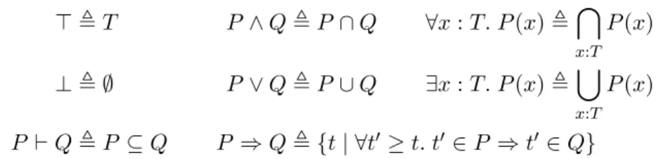
>,T P∧Q,P ∩Q ∀x:T. P(x),\ x:T P(x) ⊥,∅ P∨Q,P ∪Q ∃x:T. P(x),[ x:T P(x) P `Q,P ⊆Q P ⇒Q,{t| ∀t0 ≥t. t0 ∈P ⇒t0 ∈Q}
Figure 3: Kripke definition of a complete Heyting algebra when assertions are subsets ofT, upwards closed under a preorder ≤.
Proposition 3.1. Given a preordered type(T,≤), the powerset P≤(T) is a complete Heyting algebra, where
P≤(T),{P :P(T)| ∀t∈P.∀t0≥t. t0∈P}
and the operators of P≤(T) are defined as in Figure 3.
The definitions in Figure 3 are known as a Kripke model; the inter-esting part of it is the definition of implication, which explicitly ensures closure under≤, whereas that closure holds directly for all other operators. The injection from the metalogic to the assertion logic that was discussed in Section 3.1.2 can be defined ashpi={t|p}.
More generally, we can construct a Heyting algebra from an existing one as follows.
Proposition 3.2. Given a complete Heyting algebra A and a preordered type (T,≤), the space of monotonic functions T →≤ A is also a complete
Heyting algebra, where
T →≤A,{f :T →A| ∀t, t0. t≤t0 ⇒(f(t)`f(t0))}
and the operators of T →≤A are defined in terms of the operators on A:
P ⊕Q,λt. P(t)⊕Q(t) for ⊕ ∈ {∧,∨} P,λt.P for P∈ {>,⊥}
κx.P(x),λt. κx.P(x)(t) for κ∈ {∀,∃}
P ⇒Q,λt.∀t0 ≥t. P(t0)⇒Q(t0)
P `Q,∀t.(P(t)`Q(t))
Proof. See [BJ], Lemma ILPre ILogic.
We will use these constructions to define specification logics, and we will use generalised forms of them to define assertion logics.
∗-Assoc (P ∗Q)∗R`P∗(Q∗R) P ∗Q`Q∗P ∗-Comm ∗-emp P ∗emp ≡P P `Q ∗-` P ∗R`Q∗R P `Q−∗R ∗-Adjoint P∗Q`R P ∗Q`R −∗-Adjoint P `Q−∗R
Figure 4: Additional axioms of a BI algebra
Note that thelaw of the excluded middle, i.e.`P∨¬P for allP, does not follow from the axioms of a complete Heyting algebra, and it is invalid in the models constructed here unless the preorder is also symmetric; i.e., an equivalence relation.
3.2 BI algebras
Defining complete Heyting algebras only got us half way to separation-logic assertions. We still need an account of the operators that make separation logic special: separating conjunction (∗), separating implication (−∗), and
emp. Note that emp is sometimes writtenI in the literature.
Definition 3.2. A complete BI algebra [Pym02] is a complete Heyting algebra with additional operators (∗,−∗,emp) satisfying the axioms in Fig-ure 4. Theprecedenceof operators used in this text will be, in decreasing order:
= ∗ ∧ ∨ −∗ ⇒ ∀ ∃ ` ≡
The axioms in Figure 4 are intentionally minimal. Rules for associativity and commutativity with≡instead of`are derivable. It can also be derived that∗ is covariant in both arguments; i.e.,
P `P0 Q`Q0 P∗Q`P0∗Q0
When I required in Section 1.2 that the assertion logic must be a com-plete BI algebra, it was not only because this gives us the rules that make separation logic intuitive to work with. It is also because it is easy to satisfy these rules. We will see in Section 3.3 how a complete BI algebra arises naturally from the memory model of a typical programming language or machine.
The operators −∗ and ⇒ are often omitted from presentations when they are not needed for the examples at hand. But even then, they play an important role in metatheory: they witness that ∗and ∧commute with existential quantification as explained in the following proposition.
Proposition 3.3. In a complete Heyting algebra with an operator ∗ satis-fying rule ∗-`, it holds that (∃x:T. P(x))∗Q` ∃x:T. P(x)∗Q if and only ifthere is an operator −∗ satisfying the rules ∗-Adjoint and −∗-Adjoint.
This proposition is a direct consequence of theadjoint functor theoremin category theory, but it is worth seeing the proof written out for the specific case of separation logic. Notice that the left-to-right direction, which is probably the surprising one, is only provable because the assertion logic is higher order, and we can quantify over a type T that represents a set of assertions.
Proof. (⇐) By the following proof tree.
`-Refl ∀x.(Q(x)∗P `Q(x)∗P) ∃-R ∀x.(Q(x)∗P ` ∃x. Q(x)∗P) −∗-Adjoint ∀x.(Q(x)`P −∗ ∃x. Q(x)∗P) ∃-L ∃x. Q(x)`P −∗ ∃x. Q(x)∗P ∗-Adjoint (∃x. Q(x))∗P ` ∃x. Q(x)∗P
(⇒) Define Q −∗ R as ∃P0 : {P0 | P0 ∗Q ` R}. P0. We first prove −∗-Adjoint, which holds without appealing to the assumption we made:
`-Refl P `P P ∗Q`R (metalogic) P :{P0 |P0∗Q`R} ∃-R withP P ` ∃P0 :{P0 |P0∗Q`R}. P0 Def. P `Q−∗R
To prove∗-Adjoint, we appeal to our assumption under the name∗-∃.
P `Q−∗R ∗-` P∗Q`(Q−∗R)∗Q ∀P0.(P0∗Q`R)⇒(P0∗Q`R) (metalogic) ∀P0 :{P0 |P0∗Q`R}.(P0∗Q`R) ∃-L ∃P0 :{P0|P0∗Q`R}. P0∗Q`R ∗-∃ (∃P0 :{P0|P0∗Q`R}. P0)∗Q`R Def. (Q−∗R)∗Q`R `-Trans P∗Q`R By analogy with Proposition 3.3, we can also show that the⇒-operator exists if and only if the∧-operator commutes with existentials.
3.2.1 Classical and intuitionistic logics
There is an important special case of BI that is relevant for separation logic: Boolean BI (BBI). BBI is obtained by adding the law of the excluded middle (` P ∨ ¬P for all P) to the axioms of Figure 2, which
makes Figure 2 describe acomplete Boolean algebra – a special case of a complete Heyting algebra. Adding the axioms of Figure 4 as well, one obtains acomplete BBI algebra.
Another important dialect is affine BI [GMP05]. This is obtained by adding weakening of ∗ to BI, meaning that P ∗Q ` P, or equivalently,
emp ≡ >. It is the preferred way to define a separation logic for a garbage-collected language, where it lets us “logically forget” the resource Q with the expectation that it will be garbage-collected some time after (or even before! [Rey00, HDV11]) logically forgetting it.
In the separation-logic literature [IO01], BBI is typically known as clas-sical separation logic, and affine BI is known asintuitionistic separa-tion logic. This is unlike the more established terminology from philosoph-ical logic, where propositions that are provable in intuitionistic logic are also expected to be provable in classical logic. To add to the confusion, there also exists classical BI [BC10], which is something else entirely. To avoid these clashes of terminology, I will prefer the termsBoolean andaffine over
classical andintuitionistic in the remainder of this chapter.
A BI algebra that is both Boolean and affine collapses in the sense that
P∗Q≡P∧Q [BK10]. On the other hand, as we will see in Section 3.3.4, there exist useful separation logics that are neither Boolean nor affine.
3.2.2 Design freedom
It might seem like there is a great deal of freedom when designing a logic that satisfies the axioms in Figures 2 and 4, but many operators are in fact uniquely determined by others.
It follows from the axioms that (∗,emp), (∧,>) and (∨,⊥) are monoids. Therefore, their units are unique; this means that once the operators (∗,∧,∨) are defined, there is no freedom left to choose the operators (emp,>,⊥). Similarly, the proof rules for −∗ and ⇒ essentially say that (P −∗ −) is the right adjoint of (− ∗P) and that (P ⇒ −) is the right adjoint of (− ∧P). Since adjoints are unique, there is no freedom in choosing the operators (−∗,⇒) once (∗,∧) have been defined (and vice versa).
The quantifier∃x:T. P(x) is often thought of as an indexed disjunction
W
x:T P(x); indeed, it is sometimes formally written and treated as such
[DYBG+13]. It is therefore natural that indexed disjunction over a
two-valued type corresponds to binary disjunction (∨), and we can actually prove this, along with analogous results for∧,⊥and >:
Proposition 3.4.
1. Assume P, Q : asn, where asn is a complete Heyting algebra. Let f2:{true,false} →asn be the function that maps true to P and false
toQ. Then
P ∨Q≡ ∃b. f2(b)
P ∧Q≡ ∀b. f2(b)
2. Let f0 : ∅ → asn be the unique function with that type. Then, in a
complete Heyting algebra,
⊥ ≡ ∃x. f0(x)
> ≡ ∀x. f0(x)
Proof. See the Coq code accompanying [JBK13], SectionILogicEquiv. In summary, the operators of a complete BI algebra are determined by the relation ` and the operators (∃,∀,∗) since from the quantifiers we can get (∨,∧,⊥,>) by Proposition 3.4, and then we have⇒and−∗as the unique right adjoints of∧and ∗respectively, we haveemp as the unique unit of∗, and we have¬P defined asP ⇒ ⊥.
Using the law of the excluded middle, we can go even further and prove ∀x. P(x)≡ ¬∃x.¬P(x). This means that the operators of a completeBBI
algebra are determined by the relation`and the operators (∃,¬,∗). 3.3 Separation algebras
3.3.1 Heaps
For a typical toy programming language, the type of heaps is defined as
heap=loc *fin val, whereloc is the type of heaplocations(e.g., the natural numbers), val is the type of values that can be stored in the heap (e.g., integers and locations), and *fin is the space of partial functions with finite domain. It is convenient to let loc be an infinite set and let allheaps have finite domain because this guarantees that allocations can always succeed – there are always infinitely many free locations in the heap.
The standard way to build a complete BI algebra from this type is to define acompositionoperation: (·) :heap×heap *heap. The composition
h1·h2 is defined when the domains of h1 and h2 are disjoint, in which case
it takes the union of the two partial functions; i.e.,
(h1·h2)(l) = h1(l) ifl∈dom(h1)\dom(h2) h2(l) ifl∈dom(h2)\dom(h1) undefined otherwise
The assertion logic can then be defined as asn = P(heap), which is a complete BBI algebra with the following operators.
∃x:T. P(x) =[ x:T P(x) (1) ∀x:T. P(x) =\ x:T P(x) (2) P ∗Q={h1·h2 |h1 ∈P ∧h2∈Q} (3)
To make this useful, we define a points-to operator asl7→v={[l7→v]}, where [l7→v] is the singleton map that only mapsl tov.
Although we could in principle reason directly about heaps and their composition [NVB10], it is typically considered easier to work in terms of the total operator∗than the partial operator·. The∗operator also generalises better than ·, as we will see in Section 3.3.4.
Affine assertion logic. The assertion logic defined in Equations (1–3) is Boolean in the sense described in Section 3.2.1. More generally, for any set
X, its powerset P(X) is a complete Boolean algebra with the quantifiers defined as in (1) and (2). To build an affine logic instead of a Boolean one, we define assertions to be closed under the extension ordering of heaps, defined as h v h0 when h0 has all the same mappings as h (and possibly more).
hvh0 ,∃h0. h0 =h·h0
asn =Pv(heap)
With the same definitions of (∃,∀,∗) as in Equations (1–3), this forms a complete affine BI algebra [IO01].
3.3.2 Motivations for generalisation
Other programming languages might defineheap differently. For example, an object-oriented language [BJSB11] might haveheap=loc×field *fin val, wherefield is the set of field names; i.e., strings. A machine language for a 32-bit machine [JBK13] might haveheap = [0..232)*fin [0..28).
Furthermore, memory models are often instrumented, either at the level of operational semantics or at the logical level. An important exam-ple of such instrumentation is fractional permissions [BCOP05, Boy03], where a heap cell contains not only a value but also a rational number in
perm = {q : Q | 0 < q ≤ 1}, where permission 1 is a read-write
permis-sion, and any smaller number is a read-only permission. Then we write
heap=loc *fin val×perm and let heap composition (·) be defined even when there is overlap in the heap domains as long as the overlapping locations agree on values, and their permissions sum up to at most 1.
Very elaborately-instrumented heaps can be found in the work on con-current abstract predicates[DYDG+10, SBP13, SB13a]. These “heaps” can contain fractions, named regions, relations on (simpler) heaps, state machines, step-indexes [AM01] and ghost state.
There is thus clearly a need to construct complete BI algebras from the powersets of very elaborate structures. The good news is that there is a theory for doing exactly that in two steps: first, prove that the structure in question is a separation algebra. Then invoke a theorem that says that the powerset of any separation algebra, possibly closed under a suitable preorder, is a complete BI algebra. Proving that something is a separation algebra is often a very syntax-directed activity, so this approach greatly reduces the amount of work to be carried out when building an assertion logic.
We will first look at how to build a complete BI algebra from a separation algebra, and then we will look at how to build a separation algebra.
3.3.3 Definitions of separation algebra
The claim from Section 3.3.1 that the powerset ofloc *fin val is a complete BI algebra can be proved entirely based on the abstract properties of the composition operator (·): it forms apartial commutative monoid. Being a monoid means that composition is associative, which lifts to powersets and lets us prove associativity of the∗operator as we defined it in Equation (3). It also means that there is a unit element 0, and we can define emp ={0} and prove that it is the unit of∗. Commutativity lifts to powersets as well. The remaining rules in Figure 4 follow from (3) without appealing to the monoid properties.
The termseparation algebrais used in the literature to describe struc-tures of this kind. Unfortunately, there is little agreement on what a separa-tion algebra is precisely. Some authors [JB12, GBC11] define it as a partial commutative monoid (Σ,·,0) with a carrier setΣ, a partial binary operation (·) and a unit 0 for that operation, but the following variations, and more, exist.
• The original definition [COY07] required cancellativity, meaning that ifa1·aand a2·aare defined and equal, thena1 =a2. This
prop-erty is not important for constructing a complete BI algebra, but it can be important for validating the conjunction rule, which says that {P}c{Q1} and{P}c{Q2}implies{P}c{Q1∧Q2}[JB11, GBC11].
It is still common for definitions of separation algebras to include can-cellativity [Tue09, DHA09, BJSB11, BK10], but it is less common that they make active use of that axiom.
• Newer definitions [DHA09, BK10, DYBG+13] allow multiple units, where the intuition is that every element is associated with exactly one
unit, but there does not have to be one unit that is compatible with every element. This effectively partitions the separation algebra into equivalence classes; one for each unit. This situation arises naturally when taking the disjoint union of two single-unit separation algebras – then there will be two units [DHA09].
• Pottier [Pot13] does not require there to be units but instead requires that there is a core for every element. Ordering elements by the extension order, the core of ais meant to be the largest duplicable element less than a, where an element is duplicable if it composes with itself to yield itself. This definition does not generalise partial commutative monoids; it is something different.
• Working with a partial monoid can be awkward. Asserting definedness of composition can be overly verbose when done explicitly [NVB10] and potentially ambiguous when done implicitly [JB12]. Some authors have addressed this by requiring a total (i.e., ordinary) commutative monoid and adding an absorbing element to represent undefinedness, either always [GMP05] or when necessary [KTDG12].
• Other authors have gone in the opposite direction [GMP05, GLW06, Pot13] and generalised the composition to have typeΣ×Σ→ P(Σ). This is called a non-deterministic monoid or, in the equivalent presentation of a composition with typeP(Σ×Σ×Σ), a relational monoid.
• Dockins et al. [DHA09] proposed several more axioms that limit the class of separation algebras to those that resemble heaps in various senses.
In very recent work, Brotherston and Villard [BV13] propose a definition that generalises all of the above, except possibly Pottier’s “core” concept: Definition 3.3. Aseparation algebrais a triple (Σ,·, U) where (·) :Σ×
Σ→ P(Σ) andU ⊆Σ, and the following holds 1. Commutativity: a∈a1·a2 ⇒a∈a2·a1
2. Assoc.: a12∈a1·a2∧a123 ∈a12·a3⇒ ∃a23∈a2·a3. a123∈a1·a23
3. Existence of unit: ∀a.∃u∈U. a∈u·a
4. Minimality of unit: u∈U∧a0 ∈u·a⇒a=a0 This definition is identical to the one in the Views framework [DYBG+13] except that our composition is non-deterministic in the above sense. We will use this definition in the rest of this section to show several ways to construct a complete BI algebra from it.
The four axioms of Definition 3.3 may not look like a natural or obvious definition, but consider a lifting of·to setsA⊆Σ:
A1·A2 ,{a| ∃a1∈A1.∃a2∈A2. a∈a1·a2}
The axioms of Definition 3.3 are then equivalent to this lifted ·being com-mutative and associative with unit U.
3.3.4 Upwards-closed assertions
All assertion logics I have encountered in the literature are essentially mod-elled as the powerset of some separation algebra Σ, upwards closed under some preorder≤. That is, assertions are of type
P≤(Σ),{P :P(Σ)| ∀a∈P.∀a0≥a. a0 ∈P}
The Heyting part of the logic is then a standard Kripke semantics as defined in Figure 3 (page 12).
Typical choices of the preorder are
• Equality (=), in which caseP≤ =P(Σ), and the law of the excluded middle holds in the logic.
• Some other equivalence relation (≡), in which case the law of the excluded middle also holds.
• Theextension orderingon the separation algebra (v). We encoun-tered the extension ordering for heaps in Section 3.3.1, and it can be generalised to arbitrary separation algebras as
ava0 ,∃a0. a0 ∈a·a0
As we will see below, this leads to an affine assertion logic.
• Aninterference relation[DYDG+10, DYBG+13] that describes how other threads may modify the state described by assertions. This enables local reasoning in a concurrent setting, at the cost of precision of the assertions.
As a simple example [SBP13], a memory location could be tagged as containing a monotonic counter, which can be increased or read by any thread at any time. The interference relation is then chosen to allow for such counters to go up but not down, which means that assertions can only express that the counter has at least value n but notexactly valuen.
Another example is to let≤model the actions of a garbage collector, such as deallocating and moving objects in memory [HDV11]. Asser-tions closed under such a relation would be guaranteed immune to garbage collection.
While the Heyting part of P≤(Σ) is always as in Figure 3, there are at least two different ways to obtain the BI part, depending on how the separation algebra interacts with the preorder. The first is adapted from [DYBG+13]:
Proposition 3.5. If (Σ,·, U) is a separation algebra and ≤ is a preorder onΣ satisfying the following two conditions
1. The unit set is closed under the preorder; i.e.,∀u∈U.∀a≥u. a∈U. 2. ∀a1, a2. ∀a ∈ a1 ·a2. ∀a0 ≥ a. ∃a01 ≥ a1. ∃a02 ≥ a2. a0 ∈ a01 ·a02;
intuitively, the operands of · can be transported upwards along ≤ to follow the result.
then a complete BI algebra is formed by P≤(Σ) with the operators defined as in Figure 3 and
emp=U
P∗Q={a| ∃a1 ∈P.∃a2∈Q. a∈a1·a2}
P −∗Q={a2| ∀a02 ≥a2.∀a1 ∈P. a1·a02⊆Q}
Proof. See [BJ], Section BIViews. That proof is actually of a slightly more general fact, analogous to how Proposition 3.2 generalises Proposition 3.1. If the conditions for Proposition 3.5 are not satisfied3, then the following proposition might apply instead. It is adapted from [GMP02, POY04] and generalised from its original setting of partial commutative monoids to our setting of more general separation algebras.
Proposition 3.6. If (Σ,·, U) is a separation algebra and ≤ is a preorder onΣ satisfying the following condition
1. ∀a01, a02. ∀a0 ∈ a01 ·a02. ∀a1 ≤ a01. ∀a2 ≤ a02. ∃a ≤ a0. a ∈ a1 ·a2;
intuitively, the result of · can be transported downwards along ≤ to follow the operands.
then a complete BI algebra is formed by P≤(Σ) with the operators defined as in Figure 3 and
emp={a0| ∃u∈U. u≤a0}
P∗Q={a0| ∃a1 ∈P.∃a2 ∈Q.∃a∈a1·a2. a≤a0}
P −∗Q={a2| ∀a1 ∈P. a1·a2 ⊆Q}
Proof. See [BJ], SectionBISepRel.
3
The conditions of neither Proposition 3.5 nor Proposition 3.6 generalise the conditions of the other, so perhaps a unifying theorem is still waiting to be discovered. Notice that Proposition 3.5 gives a simple and standard definition of∗but a more involved definition of−∗, while in Proposition 3.6 it is the other way around.
Proposition 3.6 has the following corollaries for special cases of ≤. Corollary 3.1. If(Σ,·, U)is a separation algebra, then a completeBoolean
BI algebra is formed by P(Σ) with the operators defined as in Figure 3 and emp ≡U
P∗Q≡ {a| ∃a1 ∈P.∃a2 ∈Q. a∈a1·a2}
P −∗Q≡ {a2 | ∀a1 ∈P.∀a∈a1·a2. a∈Q}
P ⇒Q≡ {a|a∈P ⇒a∈Q}
Corollary 3.2. If (Σ,·, U) is a separation algebra with extension ordering
v, then a complete affine BI algebra is formed byPv(Σ) with the operators defined as in Figure 3 and
emp ≡ >
P∗Q≡ {a| ∃a1∈P.∃a2∈Q. a∈a1·a2}
P −∗Q≡ {a2 | ∀a1 ∈P.∀a∈a1·a2. a∈Q}
In logics modelled overP≤(Σ), primitive assertions such as points-to can typically be defined in terms of the injection · : Σ → P≤(Σ), defined as
a ,{a0 |a0 ≥a}. In words, a is the smallest set inP≤(Σ) that includes
a.
3.3.5 Constructions
In recent work on separation logic and related formalisms [JB12, KTDG12, LWN13, DYGW10], each module of the program can have its own sepa-ration algebra, so the task of verifying a module includes coming up with a separation algebra suitable for it and checking the conditions in Defini-tion 3.3. While this is already much simpler than proving that something is a complete BI algebra, we can make it even simpler still, because separation algebras are very compositional. The following proposition is adapted from [DHA09] and [JB12].
Proposition 3.7. Given separation algebras(Σ1,·1, U1)and(Σ2,·2, U2)and
an arbitrary type T,
1. The product Σ1×Σ2 is also a separation algebra with unit U1×U2
2. The tagged union Σ1 +Σ2 , ({1} ×Σ1) ∪({2} × Σ2) is also a
separation algebra with unit U1+U2 and composition as the smallest
relation satisfying(i, a)·(i, b) ={i} ×(a·ib) for i∈ {1,2}.
3. The set T can be viewed as a discrete separation algebra Tdiscr if
we define the units asU ,T and composition as the smallest relation satisfyingt·t={t}.
4. The space T →fin Σ
1 of finitely-supported functions is a separation
algebra. Being finitely supported means that only a finite number of values from the domain are mapped to non-unit values. The units are the functions mapping everything to some unit, and composition is pointwise:
U ,{f | ∀t. f(t)∈U1}
f ·g,{h| ∀t. h(t)∈f(t)·1g(t)}
Proof. See [BJ] for items 1,2,4. See [DHA09] for item 3.
The space of finitely-supported functions (→fin) has good composition properties. In particular, it allows currying, so the set (A×B) →fin Σ is isomorphic to the set A →fin (B →fin Σ). This is in contrast to the space of finite partial functions (*fin), which does not have this isomorphism [Par05] since the curried form allows distinguishing between the values [] (the empty map) and [a 7→ []] (a singleton map that maps a to the empty map). We found that proofs of deallocation in fictional separation logic [JB12, JB11] became much simpler when using (→fin) instead of (*fin).
We will in practice need more constructions than those given in Propo-sition 3.7. In fictional separation logic [JB12], we found it useful to revive the concept of a permission algebra [COY07], which is like a separation algebra but without units:
Definition 3.4. Apermission algebrais a pair (Π,·) where (·) :Π×Π→ P(Π), and the following holds
1. Commutativity: a∈a1·a2 ⇒a∈a2·a1
2. Assoc.: a12∈a1·a2∧a123 ∈a12·a3⇒ ∃a23∈a2·a3. a123∈a1·a23
A similar but more restrictive definition is given in [Hob11] and used for the same purpose: to serve as an intermediate structure when composing a separation algebra.
Proposition 3.8.
1. Permission algebras form products and tagged unions just like separa-tion algebras do.
2. A permission algebra Π together with a fresh unit element 0 can be viewed as a separation algebra (Π)0 , Π ∪ {0} with units {0} and
composition defined as in Π for non-unit elements and as 0 ·a =
a·0 ={a} in other cases.
3. Any set T can be viewed as an equality permission algebra T= if
we define composition as the smallest relation satisfyingt·t={t}. 4. Any set T can be viewed as anempty permission algebra T∅ if we
define composition ast·t0 =∅.
With these constructions, we can now redefine the heaps from Sec-tion 3.3.1 asheap ,loc →fin (val
∅)0. We have described the same separation
algebra (heap,·,[]) as before, but this time there is nothing further to define or prove. The composition operation and its properties follow syntactically from Propositions 3.7 and 3.8, and the fact thatP(heap) forms a complete BBI algebra follows from Corollary 3.1.
We can also define heaps with permissions [BCOP05, Hob11] for any permission algebraΠ asheapΠ ,loc →fin (val
=×Π)0. For further examples,
see [JB12, JB11].
As already mentioned, the study of separation algebras is still at an early stage, and the constructions presented here could soon be superseded by better ones. Not all definitions of separation algebra support all the constructions; in particular, multiple units are needed to support tagged unions and discrete separation algebras [DHA09]. For most of the alternative definitions of separation algebras discussed in Section 3.3.3, none of the constructions have been verified. One exception is [DHA09], which proposes several specialisations of separation algebras and verifies that each one is preserved by all constructions.
3.3.6 Cyclic definitions
Advanced separation logics often feature instrumented heaps that can “store” assertions. Examples of such stored assertions include the invariant asso-ciated with a storable lock [GBC+07], the operations allowed on a shared resource [DYDG+10], or the precondition of a procedure stored in memory [NS06].
A representative example of this situation, inspired by models of storable locks, could be the following attempt to define heaps:
Σ=loc →fin ((val×asn) ∅)0
If asn = P≤(Σ) as usual, then this definition becomes cyclic, with Σ in a negative position:
Σ=loc→fin ((val × P≤(Σ)) ∅)0
There is no set-theoretic solution to this equation, so it cannot be used as a definition.
A comprehensive treatment of the techniques that apply here is beyond the scope of this text, but the solutions can roughly be grouped into three types, ordered here by increasing expressiveness of the resulting logic.
1. Store a syntactic assertion [VN13, DYDG+10] or token [GBC+07] in-stead of a semantic assertion. This can work well enough for first-order theories.
2. Usestep-indexingor similar techniques [AMRV07, DHA09, BRS+11]
toguardthe recursive occurrence. This essentially creates an approx-imation of the recursively-defined heap up ton+ 1 recursive iterations, exploiting that a program that has only nsteps of execution left will not have time to observe what lies beyond that depth in the heap when a heap dereference takes one step. Specification validity then means that the program is valid for arbitrary values of thisn.
3. The separation logic can be developed in a metalogic that does not re-strict recursive occurrences to being re-strictly positive in the traditional sense. The topos of trees[BMSS12] has recently been proposed for this purpose; it allows negative occurrences as long as they are guarded by a modal operator.. In the model of the topos of trees, this modal operator is explained in terms of step-indexing, so this technique is sound for essentially the same reason as item 2 above.
See [SB13a] for a recent example of using the topos of trees as the metalogic of an impredicative concurrent separation logic.
Step-indexing in logical propositions, rather than types, are discussed in Section 4.2.2.
3.4 Program variables
We have so far discussed assertions quite abstractly, but ultimately they are of course used in pre-and postconditions of commands, and they must be able to describe the values ofprogram variables as named in the source program. The exact technique will necessarily be specific to the program-ming language, but there are some common patterns and even some reusable theory just like there was for heaps.
Using a shallow embedding gave us typed logical variables practically for free, but there is no such shortcut for program variables. Fortunately, program variables still tend to be simpler to support than logical variables since program variables tend to have a more restricted binding structure.
When every formal detail has to be right – especially when working in a proof assistant – then there are many pitfalls in the encoding of program
variables. This section surveys the techniques that have been proposed for handling program variables in various programming languages. The goal is to make program variables behave much like logical variables, which is the tradition in Hoare logic, while still retaining all the benefits of a shallow embedding.
The semantics of a programming language tends to divide the state into a heap and a stack (i.e., stack frame). Shared mutable data lives on the heap, while the content of local variables lives on the stack. Some authors use the term storeinstead of stack. Stacks in While-like toy programming languages are typically modelled asstack ,var →val. This also suffices for modelling many realistic languages such as Java [PB05, BJSB11] or assembly [CSV07, Myr10, JBK13], where the typevar is chosen as strings or register names respectively.
Other languages have more complex stacks, where a simple mapping from variables to values does not suffice. This tends to happen when the language enables access to the L-value of local variables, either with an ex-plicit address-of operation as in the C programming language, or imex-plicitly through variable capture [SBP10]. Complications may also arise in concur-rent languages, where the stack becomes shared when threads fork. Variable scoping rules in JavaScript is a whole research topic in itself [GMS12].
The rest of this section assumes that (instrumented) machine states can be modelled as stack×heap for some definition of heap. Even separation logics for the C programming language adopt this model and simply disallow access to the address of local variables [AB07, TKN07, JSP12, AM13].
Using the constructions from Section 3.3.5, there are at least two useful ways to turn the whole machine state into a separation algebra.
1. If we let stack be a discrete separation algebra, then the product
stackdiscr×heap is a separation algebra whose composition is defined
by
(s, h)∈(s1, h1)·(s2, h2) ⇐⇒ s=s1=s2∧h∈h1·h2
With a standard construction to form a complete BI algebra from
stackdiscr×heap, such as Corollary 3.1, we obtain the same definition
of∗ as in the vast majority of separation-logic texts:
P∗Q≡ {(s, h)| ∃h1, h2. h∈h1·h2∧(s, h1)∈P∧(s, h2)∈Q}
A drawback of this approach is that it typically requires a syntactic side condition on the frame rule to say that variables free in the frame
R must not be modified by the commandc:
{P}c{Q} modifies(c)∩fv(R) =∅ {P∗R}c{Q∗R}
A simple way to get rid of this side condition is to make local variables immutable [BTSY06], but this can of course be a major restriction of the programming language.
2. We can alternatively define stacks almost like heaps: stack =var →fin (val∅)0. This approach is known as variables as a resource, and
the original paper about this idea [PBC06] goes even further and adds fractional permissionsperm, definingstack =var →fin (val
=×perm)0.
With variables as a resource, we get a more aesthetically-pleasing frame rule because the syntactic side condition essentially becomes integrated into the definition of∗.
{P}c{Q} {P∗R}c{Q∗R}
This is also formally better in cases wheremodifies(c), the set of local variables potentially modified byc, is not easy to determine. This hap-pens in languages where we cannot syntactically see from a program what variables might be modified, or when that over-approximation is too coarse [JBK13, MG07].
The drawback is that the convenient similarity between program vari-ables and logical varivari-ables is lost. Program varivari-ables have to be treated like heap locations using some type of points-to predicate, which com-plicates the rules for variable assignment and conditionals [PBC06] [DYBG+13, Definition 17].
3.4.1 Open terms and lifting
The two constructions above allow us to have program variables in asser-tions, but that was only half of the problem. We also need program variables in expressions, including logical expressions that are not part of the program-ming language. For instance, we might like to assert thatn>m+ 1, where
nand mare written in a sans-serif font because they are program variables; i.e., symbols of type var.
If we are using variables as a resource, the example assertion above could be written as
∃m.m7→m∗ ∃n.n7→n∧ hn > m+ 1i.
Notice first the distinction between the variable name m and its value m, which makes the formula somewhat verbose. Syntactic sugar has been pro-posed to reduce this somewhat [PBC06], but it comes at a price: expected identities such ase1 6=e2 ≡ ¬(e1 =e2) fail to hold. On the other hand, the
verbosity is not much of a burden in assembly language, where the “pro-gram variables” are uninformative register names, and their values tend to be named differently from the registers that hold them [JBK13, MG07].
The rest of this section tries to follow the Hoare-logic tradition of refer-ring to program variables from deep inside expressions. As a first step, our example assertion ofn>m+ 1 can be written formally as
{(s, h)|s(n)> s(m) + 1},
but this is undesirable as it exposes the stack s, which increases verbosity and looks quite different from standard presentations. With some amount of syntactic sugar, it can be made practical, though [McC09].
In Charge! [BJB12, BJ], a Coq formalisation of separation logic, we distinguish betweenassertions andopen assertions, which I will denote here as
asn ,P(heap) and open asn ,stack →asn
respectively. The type open asn is a complete BI algebra, and it is in fact isomorphic4 toP(stackdiscr×heap). In general:
Proposition 3.9. Given a complete BI algebra A and a preordered type
(T,≤), the space of monotonic functions T →≤ A is a complete BI algebra,
where
T →≤A,{f :T →A| ∀t, t0. t≤t0 ⇒(f(t)`f(t0))}
and the operators of T →≤A are defined in terms of the operators on A:
P∗Q,λt. P(t)∗Q(t)
emp ,λt.emp
P −∗Q,λt.∀t0 ≥t. P(t0)−∗Q(t0)
The Heyting operators are defined as in Proposition 3.2 (page 12).
Proof. See [BJ], Lemma BILPreLogic.
We can extend the definition of open asn to arbitrary types T:
open T ,stack →T
This allows us to give a uniform treatment of free variables and substitutions on open terms regardless of their type. We canlift functions to work on open terms, ranged over byo:
Definition 3.5. Given an n-ary function f : (T1 × · · · ×Tn) → T, define
˙
f : (openT1× · · · ×openTn)→openT as
˙
f(o1, . . . , on),λs. f(o1(s), . . . , on(s)).
We lift constants t : T to ˙t : open T, by taking n = 0 above. Finally, we overload the same notation to mean something different for program variables x:var, defining ˙x:open val as ˙x,λs. s(x).
4
They are isomorphic as complete BI algebras, meaning that the isomorphism preserves all operators.
Returning to our example assertion, we may now write it formally as ˙
n>˙ m˙ + ˙1˙ .
We can just as easily lift functions from the metalogic that do not also exist as programming-language expressions; for instance, given fac :N→ N, we
can express that variable n holds the factorial of variablemas ˙
n= ˙˙ fac( ˙m).
As a final and important example, we can lift operators on types that have no representation in the programming language; e.g.,list cons and recursively-definedlist predicates [BJB12]. This lets us give a satisfying formal account of how we reason with arbitrary mathematics inside assertions, without im-plicitly assuming that the theories we need have been reconstructed from scratch withinopen asn.
While the benefits of open T presented thus far could be dismissed as being superficial, we found in [BJSB11]5 that the lifting concept was cru-cial for harnessing the abstraction and modularity benefits of higher-order
separation logic. It is a standard pattern of specification in higher-order separation logic to quantify and parametrise over assertion-logic predicates [BBTS05, PB08, BJSB11]. This means that formulas tend to involve opaque predicatesF, and eventually we will have to ask what are the free variables of, say, F(e). One would hope that fv(F(e))⊆ fv(e), but this depends on the definition ofF. Examples of “undisciplined”F include
F(e) =e= ˙˙ x F(e) =e[y/x] ˙= ˙0
F(e) =hx∈fv(e)i
If there is only one type of assertions,P(stack×heap), then it is difficult to statically rule out such undesired values in a shallow embedding. See the discussions in [App06], where side conditions about free variables and sub-stitutions have to be carried around with predicates. In contrast, the lifting approach always gives us well-behaved free variables and substitutions. The following two subsections will define semantic notions of free variables and substitutions such that the following holds:
fv( ˙f(o1, . . . , on))⊆fv(o1)∪. . .∪fv(on)
˙
f(o1, . . . , on)[¯e/x¯] = ˙f(o1[¯e/x¯], . . . , on[¯e/x¯])
For further examples and motivation, see [BJSB11, BJB12].
5
3.4.2 Free variables
Following Appel et al. [AB07], we can characterise free variables semantically by saying thatxis free ino:openT when a change toxcan cause a change too:
fv(o),{x| ∃s, v. o(s)6=o(s[x:=v])}
An open term can have an infinite number of free variables; for instance, every variable is free in∀x:var.x˙= ˙0. We might like to forbid such terms,˙ but it can be hard to do without restricting expressiveness, and it turns out we do not need to. Compare this to nominal logic [Pit01], which is much more well-behaved. There, open terms have a finite number of free variables and elegant support for binders in the programming language, but the approach requires the entire metalogic to be replaced.
The definition offvsatisfies convenient rules for how it applies to pointwise-lifted functions and to variables:
fv( ˙f(o1, . . . , on))⊆fv(o1)∪. . .∪fv(on)
fv( ˙x)⊆ {x}
The property on ˙f only holds with inclusion, not equality, since a variable may not be semantically free even if it occurs in an expression – for instance,
fv( ˙x−˙ x˙) =∅. The property on ˙xof course holds with equality for any non-trivial choice ofval.
3.4.3 Substitutions
It is standard, both in deep and shallow embeddings, to define a substitution
ρ:subst as a function from variables to expressions, which here means
subst ,var →open val
Expressions, ranged over by e, are of type open val in their shallowly-embedded form. A simultaneous substitution of n distinct variables can be defined as [e1, . . . , en/ x1, . . . , xn],λx. ( ei ifx=xi for somei ˙ x otherwise
We can then define a semantic notion of applying a substitution to an open term. This is written here with postfix notation as per tradition, and it is defined in terms of applying a substitution to a stack.
oρ,λs. o(sρ), where
From these definitions, we can prove as lemmas how substitution acts on pointwise-lifted functions and on variables.
( ˙f(o1, . . . , on))ρ = ˙f(o1ρ, . . . , onρ)
( ˙x)ρ =ρ(x)
Contrast this to how substitutions work in a deep embedding: the lem-mas above about howρacts on ˙f and ˙xwould be taken as thedefinition of substitution on syntactic terms, and ourdefinition of oρ would instead be proved as a lemma [SBP09, Lemma 10] [Kri12, Lemma 28.2.a.ii].
3.4.4 Typed values
Separation logic is often applied to typed programming languages such as Java [Par05, BJSB11] or C [TKN07, AB07]. The typical approach is then to generalise the syntax and operational semantics to remove static types and let the separation logic enforce typing instead – a program logic generalises a simple type system, so it is a burden to have both. It is standard [Rey02, AB07, McC09, TSFC09, SBP10, BJSB11] to do as we have been doing since Section 3.3.1 and define a type val as a tagged union of integers, pointers, Booleans and any other types that can be stored in local variables or on the heap.
The question is then whether an arithmetic operator, such as >, should have typeval×val →val orint×int →bool. In the first approach, we can immediately write logic expressions such as ˙x>˙ y˙, and the types will match up. On the other hand, we need to have an answer for how to compare, say, a pointer with a Boolean, even though such a comparison could never happen in the original, typed, programming language. This issue extends to any other operator we want to lift from the metalogic.
In the other approach, where (>) : int ×int → bool, we cannot write ˙
x>˙ y˙, since ˙>has type open int×open int →open bool while ˙xand ˙yhave typeopen val. One option is to read variables not as an untyped ˙x:open val
but as a typed intvar(x) : open int etc. Then we can write intvar(x) ˙> intvar(y). The problem that avalue could have an unexpected type is now replaced with the problem that avariable can have an unexpected type, and
intvar will have to return a dummy value, such as 0, if it reads a non-int. We have tried both approaches in Charge! [BJSB11, BJB12], and they both ended up littering specifications and proofs with distracting coercions in and out ofval.
A third approach is to make expression evaluation partial [PBC06, AB07], but this has its own set of problems; for instance, expected identities such as e1 6= e2 ≡ ¬(e1 = e2) no longer hold [PBC06]; here, (6=,=) are partial
expressions, and ¬ is from the assertion logic. Despite this, many authors model stacks as partial functions without explaining what happens when lookup fails.
It is worth looking at two separation logics that are not affected by these problems at all, even down to the last formal detail.
• In [JBK13, KBJD13], we define a separation logic for x86 machine code. Assertions are of typeP(Σ), where
Σ= (register →fin (DWORD ∅)0)×
(flag→fin (bool ∅)0)×
(DWORD →fin (BYTE ∅)0)
The three components in the product denote CPU registers, CPU flags and main memory respectively; types BYTE and DWORD denote
bool8 andbool32 respectively.
The registers and flags together can be thought of as the local variables – thestack, in our current terminology – and this stack can store both
DWORD and bool values. The separation-algebra annotations on Σ
reveal that we are using the variables-as-a-resource approach, but this is not the essence of why types on the stack work out here. It works because there is a separate name space for the registers and flags; i.e.,
EAX is a register, and it is clear from its name only that it holds a DWORD and not a bool. This approach can also work in more conventional programming languages [CGZ05].
The main memory can be thought of as theheap in our current termi-nology. Types on the heap work out for a completely different reason than for the stack. To let us store other things thanBYTEs in mem-ory, there is essentially a points-to predicate 7→T for every type T
that has a defined decoding from byte sequences to T. Then l7→T v
holds whenv:T, and the memory contents starting atldecodes tov. See also [TKN07, AM13] for related approaches with slightly different goals.
• Another approach is to not replace the type system with a program logic but insteadextend the type system until it becomes as powerful as a program logic. Programming-language terms with side effects, such as heap write, are given a type describing those effects, such as {P}{Q}, where P and Q can refer to program variables. Logical entailment is encoded as subtyping.
Examples include [BTSY06, NAMB07, Pot08, KTDG12]. Since this requires either a deep embedding or reverification of the whole metathe-ory [NMS+08, CMM+09], we lose the advantages gained from having a shallow embedding. Features such as higher kinds and dependent types must be re-created within the type system rather than borrowed from the metalogic. See also the discussion in Section 4.3.2.
The unproblematic logics mentioned above have one thing in common: they do not define a val type, but instead they keep all programming-language types explicit and separate.
The problem also seems to go away when using variables as a resource. Recall the example from Section 3.4.1, where we wrote
∃m.m7→m∗ ∃n.n7→n∧ hn > m+ 1i.
In a setting where the injection fromint toval is calledintval, we can write this assertion more explicitly as
∃m:int.m7→intval(m)∗ ∃n:int.n7→intval(n)∧ hn > m+ 1i.
This solves the problem and can be useful for any type T with an injective functionT →val. On the other hand, variables as a resource remains very verbose and does not look like standard Hoare logic.
The above pattern for getting typed program variables using a stack
version of points-to predicate will work just as well for any standard heap
points-to predicate. Since separation logic, with very few exceptions [SJP10, PS12], forbids direct heap references in expressions, we are already forced into this pattern of existential quantification and distinction between a heap location and its value, so this may as well be used to get stronger typing.
4
Specifications
The primitive unit of specification in separation logic is usually theHoare triple. In the most basic form, in a shallow embedding, the triple is a predicate in the metalogic. Section 4.1 discusses definitions and inference rules for the triple based on this assumption.
Section 4.2 will demonstrate benefits and techniques for considering the triple instead as a formula of specification logic[Rey82], which allows us to give a logical account of the context in which a given triple holds. 4.1 Hoare triples
4.1.1 Definitions
The Hoare triple is where the assertion logic from Section 3 meets the oper-ational semantics from Section 2. The Hoare triple forpartial correctness is usually defined to mean, intuitively, “for any state satisfying the precondi-tion, no execution from that state will crash, and anyterminating execution from that state will result in a state satisfying the postcondition”. In the most basic form, the triple is defined as
{P}c{Q}1 ,∀σ ∈P.¬(σ, c fail)∧