Pricing of Arithmetic Asian Quanto-Basket Options

Helsinki University of Technology

Faculty of Information and Natural Sciences Department of Mathematics and Systems Analysis

Mat-2.4108 Independent research projects in applied mathematics

Pricing of Arithmetic Asian Quanto-Basket Options

Tanja Eronen 60020W 4.9.2008

Table of contents

1 Introduction... 1

2 The Asian Quanto-Basket Option ... 4

3 Pricing an Asian Quanto-Basket Option ... 5

3.1 The Asian Quanto-Basket Call Option Price ... 8

4 Analytical Approximations... 9

4.1 Edgeworth Expansion around the Lognormal Distribution ... 10

4.2 Edgeworth Expansion around the Inverse Gamma Distribution... 14

5 Performance Analysis of Approximations ... 16

1

1 Introduction

Since the beginning of the 1980’s, there have been many innovations in the world of derivatives and the more complex option contracts were developed, called the exotic options. The use of derivatives in risk management activities has evolved rapidly since the early 1990 and derivatives are now the most important tool to manage financial risk, but hedging and portfolio management require ever increasing amount of flexibility and efficiency for the financial instruments. With that development, the number as well as the complexity of the instruments proposed to manage risk have been steadily increasing.

The Asian option is a financial option whose value depends on the average of the underlying asset during a given time interval. Asian options can use arithmetic or geometric average, but the arithmetic average is commonly used. Asian options are very frequently traded over-the-counter derivatives. Milevsky and Posner (1998a) stated that the outstanding volume is ranged from 5 to 10 billion U.S. dollars. Asian options are one of the most commonly used path dependent options. Path dependence mean that the payoffs of the options are determined by the path of the asset’s price. The payoff of basket options depend on the value of a basket of assets and it is usually a weighted arithmetic average of the underlying assets. They offer the flexibility for the simultaneous management of exposures on virtually any number and any kind of assets, and hence can satisfy the specific risk exposure hedging needs. Because the averaging generally decreases the variance of the variable, the basket options become normally cheaper than a similar portfolio of standard options. In practice, basket options are designed specifically to meet the needs of the buyer and they are traded over-the-counter.

With the Asian and basket options comes the problem to price them efficiently and accurately. Because they have particular characteristics, the famous pricing formula introduced by Black and Scholes (1973) is inadequate. The method of Black and Scholes requires the standard lognormality assumption and the arithmetic Asian and basket feature of this option lead to an expression that cannot be solved analytically. In Asian and basket options there is a sum of lognormal random

2 variables that is not lognormal. In such cases the generalisation and adjustment are needed to attain pricing techniques and approximations.

Asian options are path-dependent derivatives and they are among the most difficult to price and hedge. Also the pricing of basket options is more challenging than that of standard options because there is no explicit analytical solution for the density function of a weighted sum of correlated assets. Several approaches are proposed in the literature to price Asian and basket options. They can be categorized as follows: numerical methods, upper and lower bounds and analytical approximations. Boyle (1977) introduced a Monte Carlo simulation for option pricing and since then it has been widely used. There exist also more recent development of simulation methods, see Broadie and Glasserman (1996) and Boyle, Broadie and Glasserman (1997). The simulation methods are very flexible and the theory is simple, but pricing is very time-consuming.

In this study, the Asian quanto-basket option is examined. It is somewhat more complex than pricing basket or Asian options. It is an Asian basket option, which has strike in different currency than the payoff in maturity is paid. In multinational institutions this contract is useful, because it allows participation multinational portfolios, without being affected by the foreign exchange risk. Basket feature allows for the simultaneous management of exposures on a variety of underlying commodities and Asian feature provides the same flexibility for asset flows in time. Positions that can be hedged with Asian quanto-basket options could be hedged as well with a portfolio consist of plain vanilla European options in assets and currencies, but Asian quanto-basket options provide in general less expensive alternative. This financial option thus simplifies the international hedging by joining the hedging of exchange and industry risks.

There is variety of methods in the literature for pricing suggested to price the Asian quanto-basket options. The risk management procedure in the financial industry, however, requires often to price large number of financial options quickly and with sufficient accuracy. The pricing method should also be easy to integrate to computer and risk management system. The problem with numerical methods is that adequate precision requires more computation time and since their lengthy calculation, they are often difficult to integrate the existing risk management systems, thus in the financial industry the approximate analytical solutions are often preferred.

3 Both Asian and basket option values depend on a weighted arithmetic average of asset price. Although the average is not lognormal, it can be modelled as such in several ways. The simplest models resort to approximating arithmetic average with geometric averages (see Vorst 1992 and Gentle 1993), adjusting the strike for the difference, as well as moment-matching arithmetic average within the lognormal family (Levy 1992, Milevsky and Posner 1998b). Many studies have tested the precision of these analytical approximations for either Asian or basket option, but they are typically done with small set of parameter values to make the comparison. Datey, Gauthier and Simonato (2003) examine the precision of three different types of analytical approximations for Asian quanto-basket option by doing comprehensive simulation experiment performed on a large test pool of option contracts. They state that the quality of analytical approximation is not always constant in a parameter space and they found that the Edgeworth-lognormal and Johnson type densities are the most accurate method in whole parameter space.

The main contribution of this study is to compare two analytical approximations: the Edgeworth expansion with lognormal distribution (Turnbull and Wakeman 1991) and the Edgeworth expansion with reciprocal gamma (Milevsky and Posner 1998a). The aim is to compare the accuracy of the approximation for different averaging frequencies. Datey, Gauthier and Simonato (2003) have made a general statement of accuracy of these methods and Johnson distribution (Posner and Milevsky 1998) in the whole parameter space. In the previous version of their paper, Datey, Gauthier and Simonato also examine two other approximations proposed by Vorst (1992) for Asian options and Gentle (1993) for basket options, but they were found to the inferior and that is why they are not considered in this study.

The next section explains details the Asian quanto-Basket options. Section 3 examines the risk neutral pricing model, while Section 4 proposes a theoretical framework for the two commonly used analytical approximation for prising Asian quanto-basket options, that is the Edgeworth expansion for the inverse gamma and for the lognormal distributions. After deriving approximate valuations for Asian quanto-basket options, in Section 5 the three analytical approximations are validated, by comparing them with Monte Carlo simulation. Finally, Section 6 concludes.

4

2 The Asian Quanto-Basket Option

European option is the standard option that gives the holder the right to acquire share j on a specific date for predetermined strike price K. Its payoff function is written as

Payoff at maturity = max

(

S_T( )j −K;0

)

. (1) The Asian option is a financial option whose value depends on the average of the underlying asset during a given time interval. There exist many variations of Asian options like average rate and average strike options. In the average strike option, the payoff in maturity is fixed and the strike is floating, while in the average price option, the strike is fixed and the payoff is floating. Here after, the term Asian option is used for an arithmetic average rate Asian option. In theory, it can be also distinguished between the continuous and discrete average calculation, anyway in practise, only discrete Asian options are traded, whereas the continuous average calculation is used as an approximation of traded option in majority of research papers.

Asian option protects the investor against possible ad hoc fluctuations of the underlying assets. On financial markets, the Asian option was introduced to protect the parties from stock market manipulation of underlying values on or near the expiry date of option.

The Asian option uses an average value of the underlying assets at predetermined dates t₁,...,t_mto determine the payoff. Its payoff function is as follows

Payoff at maturity = ( )       −

∑

= 0 ; 1 max 1 K S m m i j ti , (2)

and it is given in currency j.

Basket option can be seen as a European option, but the underlying is composed of several financial assets, all generally expressed in same currency. The payoff function of a basket option is given by

5 Payoff at maturity = ( ) _       −

∑

= 0 ; max 1 K S w n j j T j , (3)

where w₁,...,w_n represent the weights associated with each asset and

∑

= = n j j w 1

1. One of the main advantages of the basket option is that it allows a generally less expensive alternative to cover several underlying assets than that of purchasing a portfolio consists of each underlying asset to be covered.

Quanto option is defined in terms of an underlying to be made out in a currency other than the currency of the payment to be made upon expiry date. Its payment function is given by

Payoff at maturity = C₀( )j max

(

S_T( )j −K;0

)

, (4) where C(₀j) is the number of units of local currency by unit of foreign currency at time t = 0. The quanto option allows indirect investment in a foreign asset without being subjected to the foreign exchange risk. It can be used also to hedge against potential fluctuation in foreign securities.

Asian quanto-basket option combines the of Asian, basket and quanto options. Its total payment in a predetermined currency is as follows

Payoff at maturity = ( ) _       −

∑∑

= = 0 ; 1 max 1 1 K S w m m i n j j t j i . (5)

The weights include the fixed exchange rates.

3 Pricing an Asian Quanto-Basket Option

The Harrison and Pliska (1981) suggest computing the value of an option with the risk neutral measure, and the discount it at the risk-free rate. In the model, there exists n foreign underlying

6 securities, n exchange rates, n risk-free foreign bonds and one risk-free domestic bond. They are noted as follows

( ) ₌

{

_S( )_:t≥0

}

S j

t

j _{for the foreign underlying security j, (6)}

( ) ₌

{

_C( )_:t≥0

}

C j _tj for the exchange rate j (domestic/foreign), (7)

( )₌

{

_B( )_:t≥0

}

B j _tj for the foreign risk free bond j, (8)

( )

{

( )

}

0 : ≥

= D t

D j _tj for the domestic risk free bond. (9)

The underlying security and the exchange rates are expected to follow the lognormal distribution. Thus we apply the following hypothesis of stochastic variables

( ) ( ) ( ) ( ) n j d dt dS_tj =µ_jS_tj +σ_jS_tj W_tj =1,..., , (10) ( ) _C( )_{dt C}( )_dZ( )_{j n} dC_tj =µ_{j t}j +α_{j t}j _tj =1,..., , (11) ( ) _{r B}( )_dt dB j t j j t = j=1,…,n, (12) dt rD dD_t = _t j=1,…,n, (13)

where W ,...,( )1 W( )n and Z( )1 ,…,Z( )n are standard Brownian motions with correlations ( ) ( )

(

)

k j j t k t P W W Corr , =θ _, , (14) ( ) ( )

(

)

k j j t k t P Z Z Corr , =λ _, , (15) ( ) ( )

(

)

k j j t k t P Z W Corr , =ρ _, . (16)

7 We also suppose that the underlying security j pays a dividend at a constant rate of δ_jon a continuous basis. Then, these all stochastic processes are built on probability space

(

Ω,F,F,P

)

, where F is the filtration

{

F_t :t≥0

}

, with

( ) ( )

{

}

(

Z W s t j n

)

F j s j s t =σ ℵ, & :0≤ ≤ & ∈ 1,2,..., , (17)

and ℵ is a set of zero probability events.

In order to present the option pricing formula, we need to represent the price of the underlying asset using a risk neutral probability measure denoted as Q. Finally, it is found that risk neutral measure is unique and following stochastic differential equation defines the required processes

( )

(

)

( ) ( ) ( )j t j t j j t j j j j j j j t r S dt S dW dS = −δ −α σ ρ _, +σ ~ j=1,…,n, (18)

where −α_jσ_jρ_j,j is an adjustment term which determines the effect of the quanto feature of the option and W~( )1,...,W~( )n are standard Brownian motion under a Q probability measure and they have correlations ( ) ( )

(

)

k j j k W W Corr ~ , ~ =θ _, . (19)

The differential equation obtained is almost identical to that representing the price of underlying asset with dividend in the Black and Scholes formula. Actually, the only difference is the term

j j j jσ ρ ,

α , which reflects the quanto feature of the option. With this term the option price is adjusted to take into account the impact of the exchange rate. The Equation (19) allows us to treat options where the basket includes some securities made out in domestic currency as well as situations where numerous securities share the same currency, then we can use α_k =α_j, v_k =v_j,

( ) ( )j t k

t Z

Z = and r_k =r_j. Similarly, if security k is in domestic currency, the model contains one less exchange rate

8 ( )

(

₀k =1, _k =0, _k =0

)

v

C α . (20)

Because Equation (18) is a standard geometric Brownian motion, the solution is

( ) ( )

[

(

)

( )j

]

j j j j j j j j j t S r t W S = ₀ exp −δ −α σ ρ _, +σ ~ j=1,…n. (21)

This section represents a standard option pricing model that is widely used, but nevertheless, it includes weaknesses, like constant volatilities and interest rates. The main advantage of the model is that it supports option pricing with an acceptable accuracy in terms of empirical observations. If options expire within a relatively short period of time, like they usually do, the above-mentioned weaknesses have diminishing influence.

3.1 The Asian Quanto-Basket Call Option Price

To price of the quanto option in the basket can be computed with the Equation (21). Now, the price of the basket can be calculated with the following formula

(

)

[

A K

]

e

(

A K

) ( )

f xdx E e V_exact rt Q rt

∫

∞ ∞ − − − _{− = −} = max ,0 max ,0 , (22)

where f

( )

x represents a density function of the arithmetic average A of the underlying basket value on the predetermined dates t₁,...,t_m. The arithmetic average is

( )

∑∑

= j t jS w m A 1 1 0≤t₁ ≤...≤t_m ≤T, (23)

where the process for S_j is given by Equation (20) and where w_j is the vector of weights of the securities in the basket. In Equation (22), it is equivalent to integrating from −∞ to +∞ and integrating from 0 to +∞ since f(x)=0 for any x<0. There is no exact solution for (21) because A is sum of lognormal random variables and integral representing the density function of a sum of lognormal random variables cannot be solved analytically.

9 Lattice-based methods are commonly used for pricing options on a single asset. However, they are computationally extensive and exponentially complicated for options on multiple assets. Numerical approximation using a Monte Carlo or Quasi-Monte Carlo methods allow to achieve a value that is as accurate as preferred. The drawback of these approaches is that it requires extensive calculations although they are less time-consuming than lattice-based approaches. The analytical approximations offer a very fast method to price Asian quanto-Basket option, even if a certain amount of accuracy is lost in the process. The time-saving is an obvious advantage for real time trading.

4 Analytical Approximations

In this section, three well-known analytical approximations for the Asian quanto-basket option are examined. In order to apply moment matching -based approximations, we need to calculate the first four moments of the weighted sum of the underlying basket of option under measure Q.

Lemma 1: Under the risk neutral measure Q, the first four moments of the arithmetic mean A are respectively ( )

∑∑

( )

[

(

)

]

= = − − = m i n j i j j j j j j j j f _{w S r t} m m 1 1 , 0 1 exp 1 ρ σ α δ , (24) ( ) ( ) ( )

(

)

( )

(

)

( )

∑ ∑

= = _                   − − + + − − × = m i i n j j i i j j j j j j i i j j j j j j j j j j j j j j f t r t r S S w w m m 1 , , 1 , max , , min , , 0 0 2 2 2 1 1 2 2 1 2 2 1 2 2 2 2 2 1 2 1 2 1 1 1 1 1 1 1 2 1 2 1 exp 1 ρ σ α δ θ σ σ ρ σ α δ , (25) ( ) ( ) ( ) ( )

(

)

( )

(

)

( )

(

)

( )             − − + + − − + + + − − × =

∑ ∑

= = 3 2 1 3 3 3 3 3 3 3 2 1 3 2 3 2 2 2 1 2 2 2 2 3 2 1 3 1 3 1 2 1 2 1 1 1 1 1 1 1 3 2 1 1 2 3 3 2 1 3 2 1 , , max , , , , , , , min , , , 1 , , , , 1 0 0 0 3 3 exp 1 i i i j j j j j j i i i med j j j j j j j j j j i i i j j j j j j j j j j j j j j m i i i n j j j j j j j j j f t r t r t r S S S w w w m m ρ σ α δ θ σ σ ρ σ α δ θ σ σ θ σ σ ρ σ α δ , (26)

10 ( ) ( ) ( ) ( ) ( )

(

)

( )

(

)

( )

(

)

( )

(

)

( )               − − + + − − + + + − − + + + + − − × =

∑

∑

= = 4 3 2 1 4 4 4 4 4 4 4 3 2 1 4 3 4 3 3 3 3 3 3 3 4 3 2 1 4 3 4 3 3 2 3 2 2 2 1 2 2 2 2 4 3 2 1 4 1 4 1 3 1 3 1 2 1 2 1 1 1 1 1 1 1 4 3 2 1 1 2 3 4 4 3 2 1 4 3 2 1 , , , max , , , , 3 , , , , , 2 , , , , , , min , , , , 1 , , , , , , 1 0 0 0 0 4 4 exp 1 i i i i j j j j j j i i i i j j j j j j j j j j i i i i j j j j j j j j j j j j j j i i i i j j j j j j j j j j j j j j j j j j m i i i i n j j j j j j j j j j j j f t r t r t r t r S S S S w w w w m m ρ σ α δ θ σ σ ρ σ α δ θ σ σ θ σ σ ρ σ α δ θ σ σ θ σ σ θ σ σ ρ σ α δ ,(27)

where x

(

i₁,i₂,i₃,i₄

)

represent xth value of the decreasing ordinate quadruple

(

i₁,i₂,i₃,i₄

)

.

The lognormal distribution makes it possible to apply the following identity

(

)

[

]

_      + = + 2 exp exp 2 b a bZ a E , (28)

where Z ~ N

( )

0,1 . The moments can be derived using Equation (28). For the next approximations we adopt following notation. The expected value as per the density function g is

( )

∫

( )

∞ ∞ − = xg x dx g µ , (29)

and the central kth moment in terms of the density function g is

( )

(

( )

)

( )

∫

∞ ∞ − − = x g kg x dx g k µ ψ . (30)

4.1 Edgeworth Expansion around the Lognormal Distribution

Our first analytical approximation is based on a generalized Edgeworth expansion around the lognormal distribution. Jarrow and Rudd (1982) were the first to propose using Edgeworth expansions to solve option pricing problems. The basic idea of this method is to replace an unknown density function f

( )

⋅ with a Taylor-like expansion around an easy-to-use density function

11 denoted a

( )

⋅ . However, the Edgeworth expansions commonly lead to a function which is not a positive and unimodal. To guarantee that the approximation obtained with a truncated Edgeworth expansion is a true density function, Barton and Dennis (1952) derive special conditions on the third and fourth moments of the unknown distribution. Moreover, Ju (2002) points out that the Edgeworth expansion may diverge for some parameter values, which consequently can give incorrect prices for high volatility and long maturity options. As suggested by Turnbull and Wakeman (1991) and by Huynh (1994), the lognormal sum in Asian basket option is approximated by a lognormal distribution and an Edgeworth expansion of the fourth order is used.

( )

x

f is the true density function of Asian quanto-basket option price and a

( )

x is chosen as an approximation of f

( )

x . a

( )

x is the lognormal density function of the random variable exp

(

aˆ+bˆZ

)

, where Z ~ N

( )

0,1 . Jarrow and Rudd (1982) show that f

( )

x can be written as following Edgeworth expansion

( )

( )

( ) ( )

( )

( ) ( )

( )

( ) ( )

(

)

(

(

( )

)

(

( )

)

)

(

( ) ( )

)

( )

( )

x dx x a d dx x a d dx x a d x a x f a f a f a f a f a f ε ψ ψ ψ ψ ψ ψ ψ ψ ψ ψ + − + − + − + − − − + = 4 4 2 2 2 2 2 2 2 4 4 3 3 3 3 2 2 2 2 ! 4 3 3 3 ! 3 ! 2 , (31)

where the centered moments ψ_k( )* are defined in Equation (30) and ε

( )

x is an error term. In general, no analytical features can be connected to error term. We choose function a

( )

x such that the first two moments are equal to those of f

( )

x . Because a lognormal distribution is completely described by its first two moments, Hence aˆ and bˆ must be equal to the expression given in Equation (24) and (25). Finally, we can rewrite Equation (31) as follows

( )

( )

( ) ( )

( )

(

( ) ( )

)

( )

( )

x dx x a d dx x a d x a x f a f a f ε ψ ψ ψ ψ + − + − − = ₄ 4 4 4 3 3 3 3 ! 4 ! 3 . (32) lognormal V is defined as

12

(

) ( )

(

) ( )

( ) ( )

( )

(

( ) ( )

)

( )

( )

(

) ( )

( ) ( )

( )

(

( ) ( )

)

( )

( )

∫

∫

∫

∞ − ∞ ∞ − − ∞ ∞ − −       + − + − − − =       + − + − − − ≅ − = K a f a f rT a f a f rT rT dx x dx x a d dx x a d x a K x e dx x dx x a d dx x a d x a K x e dx x f K x e V ε ψ ψ ψ ψ ε ψ ψ ψ ψ 4 4 4 4 3 3 3 3 4 4 4 4 3 3 3 3 lognormal ! 4 ! 3 ! 4 ! 3 0 , max 0 , max .(33)

Like Jarrow and Rudd (1982) state, that the equation

(

)

( )

( )( )

K dx x a d dx dx x a d K x _j j K j j = −

∫

∞ − − 2 2 for j≥2 (34) yields

(

) ( )

( ) ( )

( ) ( )

(

( ) ( )

)

( )( )

K dx x a d K dx x da dx x a K x e V a f a f K rT 2 2 4 4 3 3 lognormal ! 4 ! 3 ψ ψ ψ ψ − + − − − =

∫

∞ − . (35)

Because the integration is performed with respect to the lognormal density, the first term in Equation (35) is the Black and Scholes formula. The centered moments of the lognormal distribution are easily derived from the first four moments of a. The third and fourth moments of the lognormal distribution needed for the Edgeworth expansion depend only on the first and second moments of the distribution and can be given as follows

( )a ( )f m b a m_{1 1} 2 ˆ ˆ exp _=       + = , (36) ( )a

(

)

( )f m b a m₂ =exp2ˆ+2ˆ2 = ₂ , (37) ( ) ( ) ( ) ( ) ( ) 3 1 2 3 1 2 2 3 2 ˆ 9 ˆ 3 exp _      =       =         + = _f f a a a m m m m b a m , (38)

13 ( )

(

)

(

( )

)

( )

(

)

( )

(

)

( )

(

)

8 1 6 2 8 1 6 2 2 4 exp4ˆ 8ˆ _f f a a a m m m m b a m = + = = , (39)

where m₁( )f and m₂( )f are respectively the first two moments of A under the risk neutral measure. Those related with f are described in lemma 1.

Thus, the following analytical approximation is obtained as a sort of Black and Scholes price adjusted for the excess skewness and the excess kurtosis from the lognormal density

( ) ( )

( )

( ) ( )

( )

K dx a d e K dx da e V V a f rT a f rT normal 2 2 4 4 3 3 1 log ! 4 ! 3 ψ ψ ψ ψ − + − − = − − , (40) where

( )

( )

(

1 1 2

)

1 e N dˆ KN dˆ V = −rT − µ , (41) b d dˆ₁ = ˆ₂+ ˆ (42)

( )

b a K d ˆ ˆ ln ˆ 2 + − = (43) ( )

(

f

)

(

( )f

)

m m a ₁ ln ₂ 2 1 ln 2 ˆ= − (44) ( )

(

f

)

(

( )f

)

m m bˆ= ln ₂ −2ln ₁ , (45)

and where a

( )

⋅ is the density function of a lognormal distribution and N

( )

⋅ is a standardized normal distribution density function.

14 4.2 Edgeworth Expansion around the Inverse Gamma Distribution

The analytical approximation derived in this section uses also an Edgeworth expansion but instead of lognormal distribution the inverse Gamma distribution is used to approximate the sum of lognormals as proposed by Milevsky and Posner (1998a). They show that with some parameters, an infinite sum of correlated lognormal random variable converge asymptotically to an inverse gamma distribution. So they suggest that the finite sum of lognormals is approximated by inverse gamma function when pricing Asian and basket options.

As the lognormal distribution, the inverse gamma density function is defined by its first two moments. Thus, we choose the gamma inverse function g~

( )

x such that the first two moments equals those of f(x). Hence, the approximation will be defined in a similar way as the one obtained in the case of lognormal distribution, that is

(

) ( )

(

)

( )

( ) ( )

( )

(

( ) ( )

)

( )

( )

(

) ( )

( ) ( )

( )

(

( ) ( )

)

( )

( )

∫

∫

∫

∞ − ∞ ∞ − − ∞ ∞ − −       + − + − − − =       + − + − − − ≅ − = K g f g f rT g f g f R rT rT dx x dx x g d dx x g d x a K x e dx x dx x g d dx x g d x g K x e dx x f K x e V ε ψ ψ ψ ψ ε ψ ψ ψ ψ 4 4 ~ 4 4 3 3 ~ 3 3 4 4 ~ 4 4 3 3 ~ 3 3 gamma ~ ! 4 ~ ! 3 ~ ! 4 ~ ! 3 0 , max 0 , max . (46)

Definition 1: The density function of a gamma random variable with parameters

(

α,β

)

,

(

α,β

)

~G X , is given by

( )

( )

0 1 > ∀ Γ = − − − x e x x g x R α β α α β . (47)

Proposition 1: The density function of the random variable Y=1/x, where X ~G

(

α,β

)

is given by

( )

( )

β α α α β y e y y g 1 1 ~ − + − Γ = , ∀y>0. (48)

15 Then it is assumed that Y will have a n inverse-gamma distribution written as X ~G

(

α,β

)

.

Proposition 2: Let X ~G

(

α,β

)

. The moments of Y are given by

[ ]

(

)(

) (

)

i Y E t _t − − − = α α α β 1 12... 1 , (49) where i<α.

Then such inverse-gamma distribution needs to be selected that its first two moments will be equal to the first four moments of A. Let

( )

(

( )

)

( )

(

( )

)

2 1 2 2 1 2 2 f f f f m m m m + − + − = α , (50) ( )

(

( )

)

( )f ( )f f f m m m m 2 1 2 1 2 − = β , (51) where ( )f m1 and ( )f

m2 are respectively the first two moments of A under the risk neutral measure. Since

(

)

~

( )

2~−

( )

₂ − ∞ = −

∫

j j j j K dx K g d K dx g d K x for j≥2 (52) then

(

) ( )

( ) ( )

( )

( ) ( )

( )

K dx g d e K dx g d e dx x g K x e V g f rT g f rT K rT gamma 2 2 ~ 4 4 ~ 3 3 ~ ! 4 ~ ! 3 ~ ψ ψ ψ ψ − + − − − = − − ∞ −

∫

. (53)

16

(

) ( )

_            −       − = − − ∞ −

∫

~ µ₁ 1 |α 1,β 1 |α,β K K K e dx x g K x e rT K rT _{G G , (54)}

where G

(

⋅|η,λ

)

is a gamma distribution function with the parameters η and λ. These parameters are determined by matching the first two moments of the exact and approximate distributions. The approximation uses the first four moments of the inverse-gamma distribution. The first and second moments are identical to those of, Y and the third and fourth moments of Y are

( ) ( )

(

( )

)

( )

(

f

)

( )f f f g m m m m m 2 2 1 2 2 1 ~ 3 2 − = , (55) ( )

(

( )

)

(

( )

)

( )

(

)

(

( )

)

(

( )

)

4 1 2 1 2 2 3 2 2 1 ~ 4 6 7 2 f f f f f g m m m m m m + − = . (56)

Thus, the below analytical pricing formula is obtained ( ) ( )

( )

( ) ( )

( )

K dx g d e K dx g d e V V g f rT g f rT gamma 2 2 ~ 4 4 ~ 3 3 2 ~ ! 4 ~ ! 3 ψ ψ ψ ψ − + − − = − − _{, (57)} where             −       − = − µ₁ 1 |α 1,β 1 |α,β 2 K KG K G e V rT , (58)

α and β as stated in the Equations (50) and (51).

5 Performance Analysis of Approximations

To confirm the numerical accuracy of two analytical approximations with different volatilities and correlations, we conduct simulation experiments. Specifically, we compare the Asian quanto-basket

17 option price obtained with the analytical approximations to the Monte Carlo price obtained with 75 000 paths.

In simulation we use basket with three underlying assets and they are equally weighted. We simulate the prices of at-the money options. The maturity of the options is 5 years. The dividend rate, domestic and foreign risk-free rates as well as correlations are also kept fixed. These are shown in Table 1.

Table 1: Fixed parameters in simulations

Constant Parameters Values

Number of securities in the basket 3

Weights

Strike Price 100

Initial underlying security price 100

Dividend rate 0.03

Domestic risk-free rate 0.05

Foreign risk-tree rate

Correlation between the security prices and exchange rates

Correlation between security prices

Maturities 5 years

[

13 13 13

]

[

]

T 03 . 0 04 . 0 03 . 0

[

]

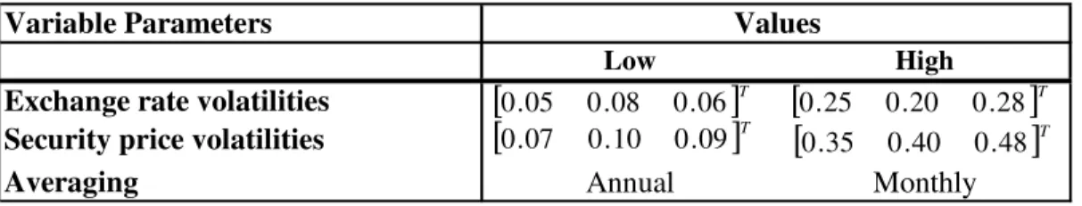
T 12 . 0 10 . 0 05 . 0           1 4 . 0 2 . 0 4 . 0 1 35 . 0 2 . 0 35 . 0 1

The priced options have monthly averaging and annual averaging. We also vary the price volatility of the underlying and exchange rate volatility. These are shown in Table 2. For these three parameters we use high and low values to be able to define if the volatilities and averaging frequency have an effect to the numerical accuracy of the approximations.

Table 2: The various parameters in simulations

Variable Parameters

Low High

Exchange rate volatilities Security price volatilities

Averaging Annual Monthly

Values

[

]

T 28 . 0 20 . 0 25 . 0

[

]

T 48 . 0 40 . 0 35 . 0

[

]

T 09 . 0 10 . 0 07 . 0

[

]

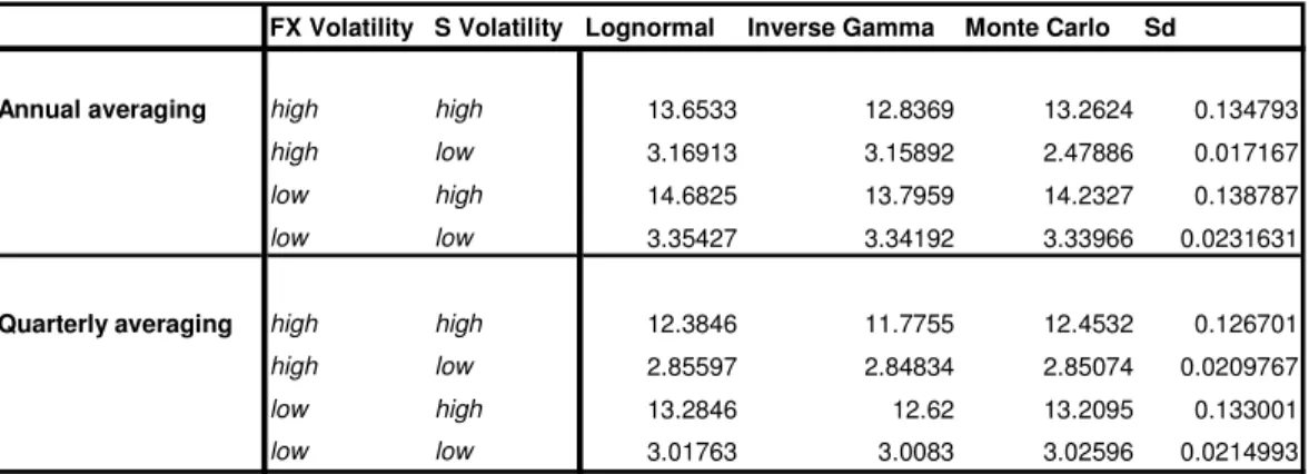
T 06 . 0 08 . 0 05 . 0

18 The Asian quanto-basket option prices calculated with Monte Carlo simulation, Edgeworth expansion using lognormal distribution and Edgeworth expansion using inverse gamma distribution are presented in Table 3.

Table 3: Asian quanto-basket option prices with different methods.

FX Volatility S Volatility Lognormal Inverse Gamma Monte Carlo Sd

Annual averaging high high 13.6533 12.8369 13.2624 0.134793

high low 3.16913 3.15892 2.47886 0.017167

low high 14.6825 13.7959 14.2327 0.138787

low low 3.35427 3.34192 3.33966 0.0231631

Quarterly averaging high high 12.3846 11.7755 12.4532 0.126701

high low 2.85597 2.84834 2.85074 0.0209767

low high 13.2846 12.62 13.2095 0.133001

low low 3.01763 3.0083 3.02596 0.0214993

The Edgeworth expansion with lognormal distribution seems to work better in the most of the parameter sets. The results are the most accurate with the small underlying securities volatilities. Especially when the volatilities of the underlying securities are high and the volatilities of the exchange rates are low, the result is inaccurate. The analytical approximations seem to be more accurate when the averaging frequency is high. This is because a continuous averaging is used to model the Asian options and the more frequent the averaging is, the more accurate the approximation will be.

6 Conclusion

Firms can use Asian quanto-basket options to hedge their exposure to different risks, such as commodity risk, interest rate risk and exchange rate risk. However, since no closed-form solution can be derived for the sum of lognormal random variables, the pricing of these options is not easy because they do not have closed form solution such as Black and Scholes. The main contribution of this study is sensitivity analysis of two analytical approximations to price the Asian quanto-basket options. We measure their sensitivity to the underlying asset price volatility and to the volatility between the underlying asset and the exchange rate. The two approximation used are the Edgeworth

19 expansion around the lognormal distribution proposed by Wakeman (1991), Edgeworth expansion around the inverse gamma distribution suggested by Milevsky and Posner (1998a).

In order to asses and compare the accuracy of the approximation we use local sensitivity analysis where the parameters of the model are fixed arbitrarily, but three of them get high and low values. Our results suggests that both approximations are accurate when the volatilities of the securities are low. When the averaging frequency is quarterly the approximations were found to be more accurate than annual averaging. This is because the continuous averaging is used to modelling the Asian options. The Edgeworth expansion using the lognormal distribution was found to be the most accurate approximation. This is inline with the previous researches.

Dionne, Gauthier, Quertani and Tahani (2006) compared three different analytical approximations for heterogeneous basket options with Monte Carlo simulation. The approximations were Inverse gamma, Edgeworth expansion around the lognormal distribution and Johnson approximation. They found that the Edgeworth-lognormal and Johnson approximation were far more accurate than the inverse gamma approximation. Detailed look at the result shows that the out-of the —money and high volatility options have the largest relative errors.

Datey, Gauthier and Simonato (2003) examined the precision of three different types of analytical approximations for Asian quanto-basket option by doing comprehensive simulation experiment performed on a large test pool of option contracts. Like they state that the quality of analytical approximation is not always constant in a parameter space and they found that the Edgeworth reciprocal gamma and Johnson type densities are the most accurate method in the whole parameter space. Extending the approach is a promising area for future research.

20

References

Barton, D. and Dennis, K., 1952. The conditions under Gram-Charlier and Edgeworth curves are positive definite and unimodal, Biometrica, 39, 425-427.

Black, F. and Scholes, M., 1973. The pricing of options and corporate liabilities. Journal of Political Economy, 81, 637-654.

Boyle, P., 1977. Options: A Monte Carlo approach. Journal of Financial Economics, 4, 323-338. Boyle, P., Broadie, M. and Glasserman, P., 1997. Monte Carlo methods for security pricing.

Journal of Economic Dynamics and Control, 21, 1267-1321.

Bröadie, M. and Glasserman, P., 1996. Estimating security price derivatives using simulation.

Management Science, 42, 269-285.

Datey, J., Gauthier, G. and Simonato, J., 2003. The performance of analytical approximations for the computation of Asian quanto-basket option prices. The Multinational Finance Journal, 7, 55-82.

Dionne, G., Gauthier G. Quertani, N. and Tahani, N., 2006. Heterogeneous basket options pricing using analytical approximations. Working paper 06-01, Centre of Research on e-Finance (CREF). (Submitted).

Gentle, D., 1993. Basket weaving. Risk 6, 5 1-52.

Harrison, M. and Pliska, S., 1981. Martingales and stochastic integrals in the theory of continuous trading. Stochastic Processes and their Applications, 11, 215-260.

Hill, I., Hill, R. and Holder, R., 1976. Fitting Johnson curves by moments. Applied Statistics, 25, 180-192.

21 Huynh, C., 1994. Back to baskets. Risk, 7, 59-61.

Jarrow, R. and Rudd, A., 1982. Approximate option valuation for arbitrary stochastic processes.

Journal of Financial Economics, 10, 347-369.

Johnson, N., 1949. Systems of frequency curves generated by methods of translation. Biometrica, 36, 149-176.

Ju, N., 2002. Pricing Asian and basket options via Taylor expansion. The Journal of Computational Finance, 5, 3, 79-103.

Levy, E., 1992. Pricing European average rate currency options. Journal of International Money and Finance, 11,474-491.

Milevsky, M. and Posner, S., 1998a. Asian options, the sum of lognormals and the reciprocal Gamma distribution. Journal of Financial and Quantitative Analysis, 33, 409-422.

Milevsky, M. and Posner, S., 1998b. A closed-form approximation for valuing basket options. The Journal of Derivatives, 6, 54-61.

Posner, S. and Milevsky, M., 1998. Valuing exotic options by approximating the SPD with higher moments. Journal of Financial Engineering, 7, 109-125.

Turnbull, S. and Wakeman, L., 1991. A quick algorithm average Asian options. Journal of Financial and Quantitative Analysis, 26, 377-389.

Vorst, T., 1992. Prices and hedge ratios of average Asian options. International Review of Financial Analysis, 1, 179-193.