Data-driven multivariate and multiscale methods for brain computer interface

(1)

and Multiscale Methods

for Brain Computer Interface

Cheolsoo Park

Supervisor : Professor Danilo P. Mandic

A Thesis submitted in fulfilment of requirements for the degree of Doctor of Philosophy of Imperial College London

Communication and Signal Processing Group Department of Electrical and Electronic Engineering

Imperial College London 2011

(2)

Abstract

This thesis focuses on the development of data-driven multivariate and multiscale meth-ods for brain computer interface (BCI) systems. The electroencephalogram (EEG), the most convenient means to measure neurophysiological activity due to its noninvasive na-ture, is mainly considered. The nonlinearity and nonstationarity inherent in EEG and its multichannel recording nature require a new set of data-driven multivariate techniques to estimate more accurately features for enhanced BCI operation. Also, a long term goal is to enable an alternative EEG recording strategy for achieving long-term and portable monitoring.

Empirical mode decomposition (EMD) and local mean decomposition (LMD), fully data-driven adaptive tools, are considered to decompose the nonlinear and nonstationary EEG signal into a set of components which are highly localised in time and frequency. It is shown that the complex and multivariate extensions of EMD, which can exploit com-mon oscillatory modes within multivariate (multichannel) data, can be used to accurately estimate and compare the amplitude and phase information among multiple sources, a key for the feature extraction of BCI system. A complex extension of local mean de-composition is also introduced and its operation is illustrated on two channel neuronal spike streams. Common spatial pattern (CSP), a standard feature extraction technique for BCI application, is also extended to complex domain using the augmented complex statistics. Depending on the circularity/noncircularity of a complex signal, one of the complex CSP algorithms can be chosen to produce the best classification performance between two different EEG classes.

Using these complex and multivariate algorithms, two cognitive brain studies are investigated for more natural and intuitive design of advanced BCI systems. Firstly,

(3)

a Yarbus-style auditory selective attention experiment is introduced to measure the user attention to a sound source among a mixture of sound stimuli, which is aimed at improving the usefulness of hearing instruments such as hearing aid. Secondly, emotion experiments elicited by taste and taste recall are examined to determine the pleasure and displeasure of a food for the implementation of affective computing. The separation between two emotional responses is examined using real and complex-valued common spatial pattern methods.

Finally, we introduce a novel approach to brain monitoring based on EEG record-ings from within the ear canal, embedded on a custom made hearing aid earplug. The new platform promises the possibility of both short- and long-term continuous use for standard brain monitoring and interfacing applications.

(4)

Acknowledgment

I would like to thank my supervisor Professor Danilo P. Mandic for his valuable guidance and support throughout the entire research, without whom this work would not have been possible. I appreciate his tolerance and thanks to him for his time spent on advising me and evaluating my work. His helps can never be forgotten.

I would like to thank Dr. David Looney, who has given me lots of inspiration and suggestion during my PhD as a good collaborator and friend.

I am also indebted to Dr. Clive Cheong-Took for his invaluable suggestions about complex-domain study, and helpful advices as a good friend.

I wish to thank my colleagues and friends with whom I had numbers of interesting discussions, in particular, Naveed Rehman, Yili Xia, Ling Li, Alireza Ahrabian, Mosabber Ahmed, Pradeep Loganathan, Jaeseung Song, Hasung Kim and Jaehwa Lee.

I also wish to thank collaborators of Widex (Denmark), Preben Kidmose, Michael Ungstrup and Mike Lind Rank for the exciting research and financial support.

Finally, to make this acknowledgement complete, a special thanks to my parents, wife Mikyung and brother for their patience and support.

(5)

List of Figures

1.1 Electrode positions in the 10-20 system. Black circles denote positions of the original 10-20 system and gray circles positions introduced in the 10-10

extension (This figure is taken from [1].). . . 28

1.2 Block diagram of a basic BCI system (adopted from [2]). . . 29

2.1 A typical intrinsic mode function. . . 39

2.2 IMFs decomposed from an EEG signal. . . 42

2.3 Time-frequency representations of frequency shift cosine waves produced us-ing STFT, Morlet wavelet and EMD (adopted from [3]). Note the localised time-frequency components in HHS. . . 43

3.1 A rotating signal of complex data and the definition of mean of envelope are presented (Figure (b) is adopted from [4]). . . 48

3.2 All the decomposed IMFs of the data in eq. (3.1) and (3.2) using EMD. The left column illustrates the decomposition of x1(t) and right column shows those of x2(t). Note the mode mixing problems across IMF7-IMF12 for both x1(t) andx2(t). . . 50

3.3 All the decomposed IMFs of the data in eq. (3.1) and (3.2) using BEMD. The left column illustrates the real parts of the complex IMFs, and the right column shows the imaginary parts of complex IMFs. Note the alleviated mode mixing problems compared to EMD results in Fig. 3.2. . . 51

(9)

3.4 Comparison between IMFs of EMD and BEMD using the data in eq. (3.1) and (3.2). EMD can decompose the original sinusoids in IMF 7 and IMF 8, and the IMF 8 and IMF 9 of BEMD include those sinusoids. Note that the decomposed IMFs using BEMD are closer to the original sinusoids than those of EMD. . . 52 3.5 HHS of EMD and BEMD for the data in eq. (3.1) and (3.2). Similarly

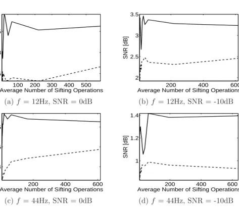
as the results in Fig. 3.4, the HHS of BEMD produces more localised and stable 13Hz and 47Hz frequency components across time. . . 52 3.6 Reconstruction results of 1Hz amplitude modulated sinusoid for different

frequencies, average number of sifting operations and SNR (‘- - -’ EMD, ‘−’ BEMD). . . 55 3.7 Direction vectors to take projections of a 3-dimensional signal on spheres

by using uniform angular sampling (a) and Hammersley sampling (b) (The figures are taken from [5].). . . 57 3.8 Averaged spectra of IMF1-IMF9 decomposed from 500 realisations of

8-channel white Gaussian noise using EMD (a) and MEMD (b) (The figures are taken from [6].). . . 58 3.9 Decomposition of a synthetic multivariate signal [a(t), b(t), c(t)], which

exhibits multiple frequency components. The common oscillatory modes are aligned at the same IMF level. However, unwanted mode mixing problem is presented in the seventh and eighth IMFs. . . 61 3.10 Decomposition of a synthetic multivariate signal [a(t), b(t), c(t), n(t)],

wheren(t)is an additional noise channel data. Note that each IMF contains a single frequency mode without mode mixing problem. . . 62 4.1 Phase synchrony spectrogram obtained for a pair of chirp signals using

BEMD [7]. . . 68 4.2 The time-frequency representations of phase synchrony for a pair of alpha

band EEG signals. The phase synchrony around alpha band by BEMD (b) is more prominent than that in the EMD result (a). . . 70 4.3 Asymmetry ratio obtained using BEMD, for two channel data in eq. (4.11) 73

(10)

4.4 The marginal Hilbert spectrum of EMD and BEMD. In all scenarios, the MHS of BEMD is more localised in frequency. . . 74 4.5 The kurtosis of the periodogram based power spectrum for a sine wave

with increasing noise levels. Kurtosis increases for high SNR, indicating a spectrum is more concentrated. . . 74 4.6 The kurtosis for the MHS of the sinusoids of frequency f obtained using

EMD (cross) and BEMD (black squares) for the different SNR. Although the kurtosis of the spectra obtained using EMD and BEMD are similar for -10dB, the results of BEMD are mostly bigger than those of EMD. The values in the square boxes are one-tailed p-values of the t-test for the kurtosis of EMD and BEMD results. . . 75 4.7 Asymmetry estimations for the alpha band signals (between the dashed

lines) in 0dB WGN. These asymmetry ratios were computed at intervals of 0.125Hz. Note that BEMD produces the lowest and most stable asymmetry in the alpha band of all the considered algorithms. . . 77 5.1 Block diagram of the role of the hearing aid within the system of

audi-tory perception which consists of: Sensory System (outer ear, middle ear, cochlear); Auditory Pathway (cochlear nucleus, auditory cortex); and Cog-nitive Layer (high level auditory layer, cogCog-nitive layer). . . 84 5.2 The Unexpected Visitor by Yarbus [8] (This figure is taken from a website

‘http://en.wikipedia.org/wiki/Eye tracking#cite ref-4’.). Notice the differ-ent patterns of eye movemdiffer-ents according to the differdiffer-ent cognitive tasks. . . 86 5.3 Simplified block diagram of brain processes in the Yarbus experiment.

Sym-bols M: motor, A: action, S: sensation, P: perception, and C: cognition. . . 87 5.4 Simplified block diagram of brain processes involved in auditory attention.

Symbols S: sensation, P: perception, and C: cognition. . . 87 5.5 ERD/ERS results for subjects ‘A’ and ‘B’ for three recording sessions

(de-noted by Rec. #). For each session, the average results for the 10 speech trials are shown in gray and the average for the 10 music trials in black. The distance between the error bars denote two standard deviations [9]. . . 94

(11)

6.1 STFT spectra for lef t hand and right hand motor imagery tasks. Left hemisphere and right hemisphere denote the average of ‘C3’ and ‘C5’, and the average of ‘C4’ and ‘C6’ respectively. . . 101 6.2 Wavelet (Morlet) spectra forlef t handandright handmotor imagery tasks.

Left hemisphere and right hemisphere denote the average of ‘C3’ and ‘C5’, and the average of ‘C4’ and ‘C6’ respectively. . . 102 6.3 EMD HHS for lef t hand and right handmotor imagery tasks. Left

hemi-sphere and right hemihemi-sphere denote the average of ‘C3’ and ‘C5’, and the average of ‘C4’ and ‘C6’ respectively. . . 102 6.4 EEMD HHS for lef t hand and right hand motor imagery tasks. Left

hemisphere and right hemisphere denote the average of ‘C3’ and ‘C5’, and the average of ‘C4’ and ‘C6’ respectively. . . 103 6.5 MEMD HHS for lef t hand and right hand motor imagery tasks. Left

hemisphere and right hemisphere denote the average of ‘C3’ and ‘C5’, and the average of ‘C4’ and ‘C6’ respectively. . . 103 6.6 Average power spectra of c1(t) - c4(t) for each subject decomposed

us-ing EMD, EEMD, MEMD and NA-MEMD. Note that the c2(t) and c3(t)

of MEMD and NA-MEMD contain the frequency bands of mu and beta rhythms respectively. . . 107 7.1 The classification performances for the taste-elicited and recall-elicited

emo-tion groups (Pleasure (P), Displeasure (D) and Neutral (N)). It is shown that a group of emotional tastes can be classified from other emotional groups.117 7.2 Features of the recall test for subject A. Dots in the white circles are support

vectors. Note that two different emotional responses are separable in the feature space. . . 119 8.1 Geometric view of circularity via ‘real-imaginary’ scatter plots: (a)

circular data with uncorrelated (circular) noise; (b) noncircular data with correlated (noncircular) noise; (c) noncircular data with uncorre-lated (circular) noise . . . 122

(12)

8.2 Classification performances of all the CSP methods and the averaged noncircularities and power differences for the corresponding data of Sub-ject E. ‘P’, ‘D’ and ‘N’ denote the pleasure, displeasure and neutral tastes. ‘AF’ is anterior-frontal channels, ‘F’ frontal channels and ‘T’ temporal chan-nels. . . 137 8.3 Classification performances of all the CSP methods and the averaged

noncircularities and power differences for the corresponding data of Sub-ject F. ‘P’, ‘D’ and ‘N’ denote the pleasure, displeasure and neutral tastes. ‘AF’ is anterior-frontal channels, ‘F’ frontal channels and ‘T’ temporal chan-nels. . . 138 8.4 Classification performances of all the CSP methods and the averaged

noncircularities and power differences for the corresponding data of Sub-ject B. ‘P’, ‘D’ and ‘N’ denote the pleasure, displeasure and neutral tastes. ‘AF’ is anterior-frontal channels, ‘F’ frontal channels and ‘T’ temporal chan-nels. . . 139 8.5 Classification performances of all the CSP methods and the averaged

noncircularities and power differences for the corresponding data of Sub-ject D. ‘P’, ‘D’ and ‘N’ denote the pleasure, displeasure and neutral tastes. ‘AF’ is anterior-frontal channels, ‘F’ frontal channels and ‘T’ temporal chan-nels. . . 140 9.1 Neuronal spike stream. The spike signal is generated with 10kHz sampling

frequency for a duration of 1 second. This neuronal spike signal has nonlin-earity, and has substantial and abrupt changes of frequency at the locations of spikes. . . 147 9.2 Comparison of LMD and EMD in the analysis of the neuronal spike signals

shown in Fig. 9.1. LMD result contains shaper and more concentrated frequency components around the spikes compared to EMD. . . 147

(13)

9.3 Complex signal composed of sine and cosine signals. The frequencies of the first two complex signals are 1kHz and the frequencies of the other two tubes are 3kHz. In addition, all of the complex signals include a 7Hz low frequency component. The grey line illustrates the local mean of the complex signal. . . 150 9.4 A PF by complex LMD consists of a frequency modulated rotation and

local magnitude function. . . 151 9.5 PFs of the complex data in Fig. 9.3. Note that PF1 has 1kHz and 3kHz

rotations contained in the original data and PF9 contains the 7Hz low frequency component. . . 152 9.6 Decomposition of a complex signal generated by combining two Duffing

waves and an additional complex low frequency trend. The first PF and IMF in real and imaginary parts contain pure Duffing waves without trend. 153 9.7 1D and 2D representations of an artificial complex signal composed of two

neuronal spike signals. . . 153 9.8 The comparison of IFs estimated by 1st PF and IMF of a complex signal

containing Duffing waves, Fig. 9.6(b) and (c). IFs derived by PF, in both the real and imaginary parts, are always closer to true values than those obtained using BEMD. . . 154 9.9 The complex PFs of spikes,z(t) =x1(t) +jx2(t), using complex LMD. . . . 155

9.10 Comparison of the time-frequency representations obtained using the real part of complex LMD and BEMD. The frequency components of the com-plex LMD provide more localised results than those using BEMD. . . 156 9.11 Comparison of the time-frequency representations obtained using the

imag-inary part of complex LMD and BEMD. The frequency components of the complex LMD provide more localised results than those using BEMD . . . 156

(14)

10.1 The commercial hearing aid and the in-the-ear electroencephalogram recording system for the left ear (ITEL) (Figure (a) was provided by WIDEX.). Two or more electrodes (ITEL1, ITEL2 and ITEL3 in this case), pointing in different directions, are mounted on a standard custom made earplug, as shown on the three projected planes. ITE electrodes were manufactured by WIDEX as a part of joint project of Imperial College London and WIDEX [10]. . . 166 10.2 ITE settings with the g.USBamp biosignal acquisition device. The ground

electrode is on the chin and reference electrode is on the right earlobe. . . 166 10.3 Alpha attenuation study (AAT). The subject was instructed to keep their

eyes open until instructed by an auditory stimulus to close the eyes after 15 s, eliciting an increase in alpha band power in both scalp and ITE electrodes [10]. . . 168

(15)

List of Tables

1.1 Signal frequency bands of EEG and corresponding consciousness levels and distributions (adopted from [11]). . . 31 3.1 Sinusoid reconstruction (ˆs_EMD(_t₎and ˆsBEMD(t)) results in SNR for different

frequencies and initial noise levels. . . 54 3.2 Reconstruction results of a 1Hz amplitude modulated sinusoid (ˆsEMD(t) and

ˆ

sBEMD(t)) in SNR for different frequencies and initial noise levels. . . 54

3.3 Reconstruction results of 2Hz Amplitude modulated sinusoid (ˆsEMD(t) and

ˆ

sBEMD(t)) in SNR for different frequencies and initial noise levels. . . 55

3.4 Sinusoid reconstruction results in SNR for different frequencies and initial noise levels. The number of ensembles for EEMD was 100. The number in the bracket next to ‘MEMD’ denotes the channel number of the decom-posed data. Note the improved performance corresponding to the increasing number of channels. . . 64 4.1 Performance indices, ρband

ρspec, for the estimation of phase synchrony between

x1(t) and x2(t). . . 69

4.2 Performance indices, ρband

ρspec, for the estimation of phase synchrony between

EEG channels. . . 70 4.3 Performance evaluation, ρband

ρspec ×100, for asymmetry estimation between

(16)

4.4 The classification rates obtained using periodogram (shown as ‘Pxx’), EMD and BEMD based on asymmetry estimation for four subjects and multiple mental task combinations (Baseline Measurement (B), Complex Problem Solving (M), Geometric Figure Rotation (R), Mental Letter Composing (L) and Visual Counting (C)). For classification, SVM with Gaussian kernel was used. Note the improved classification by the asymmetry feature obtained using BEMD. . . 80 5.1 Analogy between the original visual Yarbus experiment and the auditory

Yarbus experiment [9]. . . 89 5.2 Classification rates for 8 subjects using BEMD syncronisation (nonlinear)

and correlation (linear) features. Note the better performance of nonlinear feature [9]. . . 95 6.1 Average classification rates of 48 different scenarios based on the different

filter and feature techniques for four subjects. Morlet wavelet was used for wavelet decomposition, and the number of ensembles for EEMD was 100. Two noise channel data was added to obtain the NA-MEMD decomposition. m from eq. (6.7) defines the number of features. Note that MEMD-CSP or NA-MEMD using c2(t) andc3(t) produced the best results for all subjects. 109

6.2 Classification rates using four channel IMFs decomposed using MEMD. ‘IMF(4⊂11)’ denotes the four channel IMFs from eleven channel MEMD

de-composition. ‘IMF(4⊂4)’ is the four channel IMFs from four channel MEMD

decomposition. mfrom eq. (6.7) defines the number of features. . . 110 7.1 The classification performance for the taste-elicited emotion combinations

(Sucrose (SU), NaCl (NC), Mustard (MT), Milk Chocolate (MC), Water 1 (WT1) and Water 2 (WT2)). Note that the mean classification accuracies of five subjects exceed 70%. . . 116 7.2 The classification performance for the recall-elicited emotion combinations

(Sucrose (SU), NaCl (NC), Mustard (MT), Milk Chocolate (MC) and Water (WT)). Note that the mean classification accuracies of all subjects exceed 70% and five show higher separation rates than those of taste-elicited emotion.116

(17)

7.3 Mean values of classification performances across subjects for taste-elicited and recall-elicited emotion responses (Pleasure (P), Displeasure (D) and Neutral (N)). Note the higher separation of recall-elicited emotions than taste-elicited emotions. . . 118 8.1 ρ˙aand ˙ρb, and ˙δaand ˙δbdenote respectively thenoncircularitiesand power

differences between real and imaginary parts of complex data for Class A and B. Note the varying performance of the strictly complex CSP methods depending on the degree of circularity. . . 134 10.1 Correlation analysis between the ITE and on-scalp electrodes [10] . . . 169

(18)

Statement of Originality

Substantial parts of this thesis are believed to be original contributions to the development and assessment of multivariate and multiscale methods for brain computer interface. This thesis was not and will not be submitted to any other university or institution for fulfilling the requirements of a degree.

(19)

Publications

The following publications support the material given in this thesis,

Journal Publication:

1. C. Park, D. Looney, P. Kidmose, M.Ungstrup, and D.P. Mandic, “Time-Frequency Analysis of EEG Asymmetry using Bivariate Empirical Mode Decomposition”,IEEE Transactions on Neural Systems and Rehabilitation Engineering, vol. 19, no. 4, pp. 366-373, 2011.

2. C. Park, D. Looney, M. V. Hulle, and D. P. Mandic, “The Complex Local Mean Decomposition”,Neurocomputing, vol. 27, pp. 867-875, 2011.

(20)

Conference Publication:

1. D. Looney, C. Park, P. Kidmose, M. L. Rank, M. Ungstrup, K. Rosenkranz, and D. P. Mandic, “An In-The-Ear Platform For Recording Electroencephalogram”, In:

Proceedings of the International Conference of the IEEE Engineering in Medicine and Biology Society, 2011.

2. C. Park, D. Looney, and D. Mandic, “Estimating Human Response to Taste using EEG”, In: Proceedings of the International Conference of the IEEE Engineering in Medicine and Biology Society, 2011.

3. L. Li, D. Looney,C. Park, and D. Mandic, “Power Independent EMG based Gesture Recognition for Robotics”, In: Proceedings of the International Conference of the IEEE Engineering in Medicine and Biology Society, 2011.

4. P. Kidmose, M. L. Rank, M. Ungstrup, D. Looney,C. Park, and D.P. Mandic, “A Yarbus-Style Experiment to Determine Auditory Attention”, In: Proceedings of the International Conference of the IEEE Engineering in Medicine and Biology Society, pp. 4650-4653, 2010.

5. D. Looney, C. Park, Y. Xia, P. Kidmose, M. Ungstrup, and D.P. Mandic, “To-wards Estimating Selective Auditory Attention From EEG Using A Novel Time-Frequency-Synchronisation Framework”, In: Proceedings of IEEE World Congress on Computational Intelligence, pp. 1-5, 2009.

6. D. Looney, C. Park, P. Kidmose, M. Ungstrup, and D.P. Mandic, “Measuring Phase Synchrony using Complex Extensions of EMD”, In: Proceedings of the IEEE Statistical Signal Processing Symposium, pp. 49-52, 2009.

(21)

List of Abbreviations

3D Three dimensions

AAT Alpha attenuation test

ACCSP Augmented complex common spatial pattern ACLMS Augmented complex least mean square

ACSP Augmented common spatial pattern AM Amplitude modulation

ANS Autonomic nervous system ASSR Auditory steady-state response

BCI Brain computer interface

BEMD Bivariate empirical mode decomposition BMI Brain machine interface

CCSP Complex common spatial pattern CD Circular data

CE Conformit´e Europ´eenne

CEMD Complex empirical mode decomposition CN Correlated noise

CNS Central nervous system CSP Common spatial pattern DFT Discrete Fourier transform ECG Electrocardiogram

EDA Exploratory data analysis EEG Electroencephalography

(22)

EMD Empirical mode decomposition EOG Electrooculogram

ERD Event-related desynchronisation ERS Event-related synchronisation ERP Event-related potential

FM Frequency modulation HHS Hilbert-Huang spectrum HR Heart rate HS Hedonic score IA Instantaneous amplitude IF Instantaneous frequency IIR Infinite impulse response IMF Intrinsic mode function

ITE In-The-Ear ITEL In-The-Ear left ITER In-The-Ear right

LMD Local mean decomposition MEG Magnetoencephalography

MHS Marginal Hilbert spectra

NA-MEMD Noise-assisted multivariate empirical mode decomposition ND Noncircular data

PET Positron emission tomography PF Product function

PCV Phase coherence value

RIEMD Rotation invariant empirical mode decomposition SMR Sensorimotor rhythms

SNR Signal-to-noise ratio SPL Sound pressure level

(23)

SSVEP Steady-state visual evoked-potential STFT Short-time Fourier transform

SUT Strong-uncorrelating transform SVM Support vector machine

TFR Time frequency representation UN Uncorrelated noise

WGN White Gaussian noise WL Widely linear

(24)

List of Principal Symbols

˙

B Magnetic field vector Cxy(f) Coherence between xand y

C(·) Statistical covariance operator

Ca Augmented covariance matrix ˘

C Matrix including all the components of IMFs

C, C Covariance matrix

C _{Complex domain}

E[·] Statistical expectation operator ˜

G Whitening transformation function H(·) Hilbert transform operator

˜

H Shannon entropy

H(w, t) Hilbert-Huang spectrum I Identity matrix

N0 Expected number of extrema

N1 Expected number of zero crossings

P Cauchy principal value Pxx Periodogram

˙

Pxx Power spectral density of x ˙

Pyy Power spectral density of y ˙

Pxy Cross spectral density between x and y P Fi(t) Product function

ˆ

PP ER(f) Power spectrum using a periodogram

(25)

R phase synchrony matrix ´

R intrinsic multi-correlation matrix

R _{Real domain}

˙

S Area of the conducting loop VM I Inducted voltage in a loop

W Window length W Spatial filter

ˆ

W Augmented spatial filter ˘

W Wiener filter X Spatial covariance arctan Arctangent

arccos Arccosine

ai(t) Instantaneous amplitude function ¯

a(t) Envelope function

ci(t) IMF signal where idenotes the IMF index cov(·) Statistical covariance

cP Fi(t) Complex product function el(t) Lower envelope of a signal eu(t) Upper envelope of a signal

{eθk(t)}

K

k=1 A set of envelope curves of a complex signal

{eθk_(t)_}K

k=1 A set of multivariate envelope curves of a multivariate signal

f Frequency

fs Sampling frequency

fA(·) Amplitude modulation operation hb{·} A bandpass Butterworth filter operator

h(w) Marginal Hilbert spectrum mi The ith moment of the spectrum

{pθk_(t)_}T

t=1 A set of multivariate signal projections

{pθk}

K

(26)

p(f) Normalised power spectrum

r₍_f₁_,f₂₎ Correlation between two signals within the frequency range f1 and f2

¯

s(t) Frequency modulated signal ˙

s Order of spline

sf(t) Sinusoid of frequencyf

v(t) Realisation of white Gaussian noise

var(·) Statistical variance

wj Row vector of a spatial filter xchirp(t) Chirp signal

(·)−₁

Matrix inverse operator (·)∗

Conjugate operator

(·)H _{Conjugate transpose operator} (·)T Vector or matrix transpose operator

ℜ(·) Real part of a complex number

ℑ(·) Imaginery part of a complex number ψ∗

Basic wavelet function

α₍_f₁_,f₂₎ Degree of phase synchrony within the frequency range from f1 tof2

˙

δ Normalised power difference

γi(t) A set of M complex/bivariate IMFs θi(t) Instantaneous phase function ωi(t) Instantaneous frequency function

σ Standard deviation ˆ

σ(t) Evaluation function for the EMD stopping criterion φi(t) Instantaneous phase difference

ρi(t) Degree of the phase synchrony ˙

ρ Noncircularity coefficient

Φ(t, f) Phase synchrony information at timet and frequencyf Γ(w1,w2) Asymmetry ratio within the frequency range fromw1 tow2

Λ Diagonal matrix of eigenvalues

(27)

Chapter 1

Introduction

1.1

Overview

Brain-computer interface (BCI) is a novel research paradigm that facilitates computer-aided control using exclusively brain activity. The advances in neural devices and their application across bioengineering fields have continuously developed BCI technology. The main motivation has been to develop a neuroprosthetic system to give mobility and in-dependence to severely paralysed patients owing to spinal cord injury, brainstem stroke and neuromuscular disorders [12]. Often the paralysis is so severe that voluntary mus-cle control, such as eye movement or respiration, is lost and thus conventional prosthetic technologies which require voluntary muscle control are not suitable [13].

Recently several noninvasive methods have been used to monitor brain functions in-cluding electroencephalography (EEG), magnetoencephalography (MEG), positron emis-sion tomography (PET), and functional magnetic resonance imaging (fMRI) [13]. For a portable BCI system which can operate in real-time, EEG is the most convenient means to measure neurophysiological activity due to its high temporal resolution, and relatively simple and affordable recording equipment compared to MEG, PET and fMRI [13,14]. Fig. 1.1 illustrates the EEG electrode positions in the standard 10-20 system [1]. A spectrum of brain responses is observable using EEG which can enable BCI including the motor action response, auditory/visual steady state responses and the auditory/visual oddball

(28)

Figure 1.1: Electrode positions in the 10-20 system. Black circles denote positions of the original 10-20 system and gray circles positions introduced in the 10-10 extension (This figure is taken from [1].).

responses [15–22]. A block diagram of a BCI system is illustrated in Fig. 1.2, with four components; signal acquisition, feature extraction, translation and BCI application [2]. The recorded EEG signal in the signal acquisition part is digitized to be processed in the signal processing components - feature extraction and translation (or classification). The translated (or classified) information is sent to a BCI application, for instance a BCI-controlled wheelchair.

1.1.1 Design of BCI

The P300 (oddball paradigm) and steady-state visual evoked-potential (SSVEP) responses have been widely used in BCI applications due to their high performance and minimal user-training time [21,22]. However, both methods require an external repetitive stimulus which can cause discomfort to the user, particularly when experienced for long periods of time. Instead, it is desirable to maximise user comfort by exploiting more intuitive paradigms. For example, BCI paradigms based on auditory stimuli allow greater user comfort and user freedom, by which computer control is possible while the visual modality is occupied (while the user is driving for instance). It has been shown that binary classification can be accurately acquired when perceptually simple tones are used as auditory stimuli [23, 24].

(29)

Figure 1.2: Block diagram of a basic BCI system (adopted from [2]).

Another approach for the intuitive and natural BCI system is motor imagery BCI, which is based on the so-called sensorimotor rhythms (mu rhythms (8-12Hz) and beta rhythms (18-25Hz)) observed when subjects plan and execute their hand or finger move-ments [18, 25]. Without any external stimulus, a subject can be trained to change the amplitude of his voluntary sensorimotor rhythms. Choi and Cichocki [19] successfully built an EEG-based BCI system to control a wheelchair in real time using the motor imagery response.

Studies which aim to detect and model human emotions have received considerable attention in order to implement natural and reliable affective computing [26, 27]. EEG signals originating from the central nervous system (CNS) are expected to contain true information of emotional changes, which are caused at the unconscious level of the subject even if the subject tries to control his/her affective state. It has been shown that emotions elicited by video and voice caused consistent changes of observed EEG [28, 29]. The emotional feedback, for instance satisfaction, confusion, frustration or amusement, then provides interactive services to the users depending on their emotional states.

(30)

1.1.2 Shortcomings of EEG-based BCI

Despite the clear potential of EEG to monitor brain activity, there are several shortcomings which obstruct its widespread and practical use for BCI systems in real life:

• Standard signal processing techniques are sub-optimal for the nonlinear, nonstation-ary and multichannel nature of EEG data;

• Existing EEG recording platforms are not suitable for achieving long-term and portable monitoring in uncontrolled environments.

The above issues motivated us to investigate an alternative EEG analysis and recording strategies in this thesis.

EEG Signal Processing

Most existing studies for EEG-based BCI systems have employed standard signal process-ing techniques based on Fourier analysis [14, 17, 25, 30–33]. The conventional methods are based on a projection onto a predefined set of basis functions and thus inherit the problem of poor time-frequency localisation associated with standard spectrum estimation [3]. Ad-ditionally, the use of linear orthogonal basis functions assumes unrealistic data properties, linearity and stationarity, which make them unsuitable for the analysis of real-world EEG data which is often nonlinear and nonstationary [34]. Additionally, the short length EEG epochs used to implement real-time BCI systems tend to be more nonstationary, and the imperfection of the sensors can produce a nonlinear output even if the underlying system is linear. Therefore alternative EEG processing techniques to Fourier-based ones are a prerequisite to enable high performance BCI systems.

Data fusion describes the extraction of more accurate information by combining data from multiple sensors than can be achieved from using only a single sensor [35]. Most EEG systems record from multiple electrodes to model brain activity from all over the scalp, and features obtained by examining the relationship between these electrodes, such as coherence, correlation, asymmetry and phase synchrony, can provide valuable

(31)

Table 1.1: Signal frequency bands of EEG and corresponding consciousness levels and distributions (adopted from [11]).

Frequency Band Frequency (Hz) Consciousness Level Distribution Delta 0.5-4 Low-Level of Arousal Generally broad, diffused

Theta 4-8 Distracted Regional, involve many lobes

Alpha 8-13 Relaxed, meditation Regional, involve entire lobes Low Beta 13-15 Relaxed yet focused By side and lobe (frontal, occipital) Midrange Beta 15-18 Alert, active not agitated Localised, over various area

High Beta 18-30 Very focused, alertness Very localised, maybe very focused Gamma 30-100+ High-level info processing Very localised

information [7, 34, 36]. In particular, the common oscillatory modes existing across the channels define the change of those features corresponding to a mental activity since the different frequency bands of EEG, for example delta, theta, alpha, beta and gamma bands, reflect different brain activities [9,37–39]. The description of EEG bands corresponding to consciousness levels are described in Table 1.1. Therefore, a robust multiscale decomposi-tion technique for multichannel data is required to examine synchronised dynamics within EEG.

Two real-valued EEG spatially symmetric signals x and y can be paired to form a complex-valued data, z = x+jy. This complexification procedure allows for the cou-pling between the two channels to be exploited. For instance, phase synchrony [7] and asymmetry [34] can affect the level of noncircularity of the composed complex signal, and thus complex-valued EEG data is mostly noncircular. By considering both the pseudo-covariance E[xxT_{] and the traditional covariance} _E[xxH_{] matrix, enhanced modeling of} real-world noncircular complex signals is achieved [40, 41]. However, a conventional com-plex algorithm to model the comcom-plex-valued EEG data, for example comcom-plex extension of common spatial pattern (CSP) [42], only uses covariance matrix, which does not include all information of the noncircular data.

Long-Term EEG Recording Device

Even if there are portable types of EEG recording systems, they are still bulky with long leads connected between the head and amplifier for the use of long-term recording. Instead, small unobtrusive devices are desirable to avoid influencing EEG response by user

(32)

interference [43]. So-called wearable EEG devices are designed to be minimally intrusive, comfortable and ergonomically acceptable and to perform long-term recordings over days and weeks [43]. However, the existing wearable systems still require a cumbersome setup process. It is impossible for a user to obtain reliable setup without an assistance of a trained person using scalp-based recording devices. Correct placement of the electrodes is essential to ensure inter-session repeatability of recordings with sufficient accuracy.

1.2

Research Objectives

Recent research on signal decomposition has been based on fully data driven techniques or exploratory data analysis (EDA) [44]. One such technique is empirical mode decomposition (EMD), which decomposes the signal into a finite set of AM (amplitude modulated)/FM (frequency modulated) components [3]. EMD makes no prior assumptions about the data, and thus it is a suitable solution for the analysis of nonlinear and nonstationary phenom-ena, which will be explained in Chapter 2. Consequently, it has been successfully employed in the analysis of intracortical signals and EEG [45–48], which are often nonlinear and non-stationary. In this thesis, it is shown how EMD can be used to decompose EEG data into multiscale components and produce more robust features corresponding to neurocognitive responses compared to conventional Fourier analysis.

The real-valued EMD algorithm was extended to complex domain in [4, 49, 50], by which the complex data can be directly decomposed by taking into account interchannel coupling domain. Chapters 3, 4 and 5 address that it is advantageous to apply complex EMD to the complex data composed of a pair of real-valued data in real and imaginary parts due to the improving stability and locality of decomposition by the shared infor-mation between two data. The same advantage can be also obtained using multivariate extension of EMD for multichannel data [5], which is a generic extension of the stan-dard EMD and BEMD. Chapter 6 shows that multivariate EMD gives more localised and accurate decompositions across time and frequency for multichannel data, when they share common oscillatory components, than single channel analysis. Using the complex and multivariate extensions of EMD, more accurate features about the amplitude and

(33)

phase information for multichannel EEG data are estimated and are shown to improve the performance of BCI system.

As a fundamental study for BCI development, new neurocognitive experiments us-ing EEG are investigated and designed, and their significances are illustrated by applyus-ing the multichannel/multivariate feature extraction techniques. The auditory Yarbus exper-iment, motivated by the standard visual Yarbus experexper-iment, was designed for auditory selective attention by Kidmoseet al.[9] and its experiment results using EMD algorithms are presented in Chapter 5. BCI system developed by this study has the potential to improve the usefulness of hearing instruments such as hearing aid by providing the infor-mation of user attention to a sound source among a mixture of sound stimuli. The second neurocognitive experiment is the estimation of human emotion to implement reliable af-fective computing. In Chapter 7, the emotion elicited by taste is monitored using EEG and the response is compared against the response to the recall of the same taste.

Additionally, common spatial patterns (CSP) algorithm, commonly used for current BCI systems, is also extended to complex domain in Chapter 8. A class of complex-valued CSP algorithms is introduced to cater for signals with noncircular probability distributions, a typical case in multichannel EEG. The proposed complex-valued CSP algorithms are derived for the generality of complex data, both circular and noncircular, based on augmented complex statistics and the strong-uncorrelating transform (SUT). Depending on the degree of correlation and power difference of complex signals, that is, the degree of improperness, one of the complex CSP algorithms is shown to maximise the difference between two mental tasks.

Chapter 9 introduces the complex extensions of another data-driven decomposition algorithm, so called local mean decomposition (LMD). The smoothed local mean of the LMD surpasses the problems with the cubic spline method used by the EMD to extract amplitude and frequency modulated components. The successful application of complex LMD to multichannel neuronal spike streams is demonstrated.

(34)

(35)

Chapter 2

Empirical Mode Decomposition

E

MPIRICAL Mode Decomposition is a fully data-driven technique for decomposing the signal into amplitude modulation (AM)/frequency modulation (FM) compo-nents which reflect its natural oscillations. The EMD makes no prior assumptions on the data and, as such, it is suitable for the analysis of nonlinear and nonstationary processes. In this chapter, we shall explain the background of EMD algorithm in terms of its abil-ity to operate at the level of instantaneous frequency and show an example of the EMD decomposition on a electroencephalogram data.

2.1

Background

In pure science and practical engineering, data analysis is a indispensable part. When we construct a numerical model to a real-world data, there are several problems in the data to determine the parameters such as:

• the short length of the data span

• nonstationarity of the data

• nonlinearity of the data

Spectrum analysis, which is still used in most areas, becomes synonymous with Fourier spectral analysis due to its simplicity and calculation speed. Even though Fourier

(36)

analysis dominates most of the data analysis, it has critical restrictions when applied to a real-world data since it is designed for linear systems, and periodic and stationary data.

The stationarity of a time series X(t) in the strict sense is defined if the joint distributions of

[X(t1), X(t2), . . . , X(tn)] and [X(t1+τ), X(t2+τ), . . . , X(tn+τ)] (2.1)

are the same for allti and τ. The definition of stationarity in the wide sense is E(X(t)2

)<∞,

E(X(t)) =m, (2.2)

C(X(t1), X(t2)) =C(X(t1+τ), X(t2+τ)) =C(t1−t2)

whereE(·) is the expected value operator andC(·) is the covariance operator. Due to the limitation of data length, few data sets in real-world can satisfy this stationarity condition. In addition, most of natural phenomena tend to be nonlinear, and the imperfection of the sensors makes the final output signal nonlinear even if the system is perfectly linear.

There have been several efforts in order to deal with the nonstationary data, for instance ‘spectrogram’ and ‘wavelet analysis’. The spectrogram is a Fourier spectral anal-ysis for a time-windowed data sets. By sliding the window along all the time span, several sets of frequency spectra can be obtained, which can be combined in a time-frequency distribution. Due to its reliance on the traditional Fourier analysis, this cannot be the best solution unless the signals in every window are stationary, which is hardly expected in a real-world signal. Secondly, the wavelet analysis is basically a linear analysis and provides a uniform resolution for all the scales, which is limited by the size of the basic wavelet function [3]. The general definition of wavelet analysis is

W(a, b;X, ψ) =|a|−1/2 Z ∞ −∞ X(t)ψ∗(t−b a )dt (2.3) where ψ∗

is the basic wavelet function, a the dilation factor and b the translation of the origin. The commonly used Morlet wavelet1_{has the problem of leakage, which is generated}

1_{The Morlet wavelet is the most commonly used wavelet transform, and had been used for the} perfor-mance comparison with EMD in [3] and [51].

(37)

by the limitation of basic wavelet function length. Due to the problem, it is difficult to define the energy-frequency-time distribution quantitatively.

In this chapter, the empirical mode decomposition (EMD) method will be presented as an alternative to the conventional Fourier and wavelet analysis. The EMD is a fully data-driven operation for obtaining a highly localised time-frequency estimation for a nonlinear and nonstationary signal [3], by decomposing it into a finite set of AM/FM components, intrinsic mode functions (IMFs).

2.2

Instantaneous Frequency using Intrinsic Mode

Func-tions

Instantaneous frequency provides a physically meaningful analysis for nonstationary data. The instantaneous frequency can be obtained by making use of the Hilbert transform

Y(t) = 1 πP Z ∞ −∞ X(t′ ) t−t′dt ′ (2.4)

and exploiting the concept of an analytic signal, where symbol P indicates the Cauchy principal value and X(t) the data. Using the Cauchy principal value, eq. 2.4 can be integrated by considering the discontinuity at t′

= t Y(t) = 1 πP Z ∞ −∞ X(t′ ) t−t′dt ′ = 1 πǫlim→0 Z t−ǫ −∞ X(t′ ) t−t′dt ′ + Z ∞ t+ǫ X(t′ ) t−t′dt ′ (2.5)

Then, using the conjugate pair of X(t) and Y(t), an analytic signal Z(t) can be obtained as

Z(t) =X(t) +jY(t) =a(t)ejθ(t), (2.6) in which

a(t) = [X2(t) +Y2(t)]1/2, θ(t) =arctan(Y(t)

X(t)) (2.7)

The instantaneous frequency can be defined as ω(t) = dθ(t)

(38)

For meaningful instantaneous frequency, there is a limitation on the data - in the sense of a ‘monocomponent’ signal, which was introduced by Cohen [52], since there is only one frequency value representing one component (monocomponent) at any given time. However, there is no precise definition of the notion of ‘monocomponent’ and thus the ‘narrowband’ assumption was adopted [53]. The narrowband signal is identified when the expected number of extrema (N0) is equal to the expected number of zero crossings

(N1), such that N0 = 1 π( m2 m0 )1/2 and N1= 1 π( m4 m2 )1/2 (2.9) N₁2−N₀2= 1 π2 m4m0−m22 m2m0 = 0 (2.10)

wheremi is the ith moment of the spectrum.

Huang et al. suggested one more condition on a signal to produce a meaningful instantaneous frequency, that is, the signal ought be symmetric with respect to the local zero mean [3]. This condition is necessary to prevent the unwanted fluctuations of instan-taneous frequency caused by asymmetric wave forms. The asymmetric wave forms in a signal produce unstable instantaneous frequencies and even negative frequencies [3]. With this additional limitation on a data, Huang et al. introduced an intrinsic mode function (IMF), which satisfies the following two conditions:

• the number of extrema and the number of zero crossings differ at most by one

• the mean of the envelopes associated respectively with the local maxima and local minima must be approximately zero

The IMFs can be AM/FM components. Fig. 2.1 illustrates a typical intrinsic mode function decomposed from the electroencephalogram (EEG), where the numbers of zero crossings and extrema are the same and the upper and lower envelopes are symmetric with respect to zero.

In the next section, it is shown that a signal can be decomposed into IMF com-ponents using the empirical mode decomposition method and that an instantaneous fre-quency can be calculated for each IMF components.

(39)

0 0.5 1 1.5 2 −3 −2 −1 0 1 2 3x 10 −6 time (s) EEG Amplitude (V)

Figure 2.1: A typical intrinsic mode function.

2.3

Empirical Mode Decomposition

Since more than one oscillatory mode may be included in data, we cannot directly apply the Hilbert transform to a general data, as it would not produce the information about all the oscillatory modes [54]. Therefore, EMD was introduced by Huanget al.to decompose a signal into IMFs [3]. EMD is a fully data-driven operation for obtaining a highly localised time-frequency estimation, which can deal with a nonlinear and nonstationary signal. In the process of EMD, the intrinsic oscillatory modes are empirically identified by their own time scales in a signal, and then used to decompose the signal subsequently. The principles of the EMD operation are outlined in Algorithm 1.

(40)

Algorithm 1. The standard EMD algorithm [3] 1) Let ˜x(t) =x(t) (x(t) is original signal)

2) Identify all local maxima and minima of ˜x(t)

3) Find a lower ‘envelope’,el(t), that interpolates all local minima by a cubic spline line (the order of spline ˙s= 3)

4) Find an upper ‘envelope’,eu(t), that interpolates all local maxima by a cubic spline line

5) Calculate the local mean value using the lower and upper envelopes m(t) = (el(t) +eu(t))/2

6) Subtract the local mean valuem(t) from the data ˜x(t) d(t) = ˜x(t)−m(t)

7) Let ˜x(t) =d(t) and go to step 2); repeat until d(t) becomes an IMF, controlled by the stopping criterion

The first IMF is subtracted from the original data, r(t) =x(t)−d(t), and the procedure is applied iteratively to the residue, r(t), until it becomes constant or contains no more oscillations; this so called sifting process is controlled by the stopping criterion [55]. The stopping criterion uses the mode amplitude a(t) := (eu(t)−el(t))/2 and the evaluation function ˆσ(t) := |m(t)/a(t)|, so that the sifting process is iterated until ˆσ(t) < θ1 for

some prescribed fraction (1- ˙α) of the total duration, while ˆσ(t) < θ2 for the remaining

fraction [55]. The default value of [θ1,θ2, ˙α] is [0.05, 0.5, 0.05]. The signalx(t) decomposed

by the EMD algorithm can thus be written as

x(t) = M

X

i=1

ci(t) +r(t) (2.11)

where ci(t), i= 1, . . . , M, is the set of IMFs andr(t) the remaining residue. Due to the narrowband nature of the IMFs, the Hilbert transform can be applied in order to obtain a localised instantaneous frequency for a time-frequency spectrum. Using the Hilbert

(41)

transform in eq. (2.4), an IMF ci(t) is represented as an analytic signal such that X(t) = M X i=1 (ci(t) +jH(ci(t))) = M X i=1 ai(t)ejθi(t) (2.12)

and the analytic form of the IMF is described by its amplitude and phase functions, ai(t) and θi(t). Using eq. (2.8), the instantaneous frequency can be produced. A plot of the amplitude ai(t) versus time t and instantaneous frequency wi(t), that is, amplitude con-tours on the time-frequency plane, is called the Hilbert-Huang spectrum (HHS), H(w, t), and represents a three dimensional time-frequency spectrum of the signal.

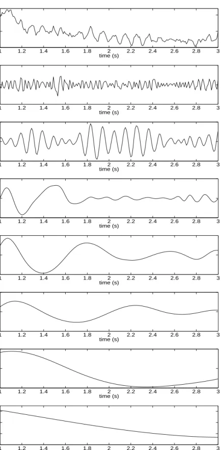
Fig. 2.2 shows all the decomposed IMFs of an EEG signal. Observe that the first IMF, c1(t), contains the fastest oscillation and the last one, r(t), involves the slowest

oscillation of the EEG trend. The seven IMFs were defined adaptively from the data without any predefined basis function like Fourier analysis, by which the nonstationary and nonlinear EEG data was well decomposed. In order to investigate the power resolution of the HHS, we considered frequency shift cosine waves shown in Fig. 2.3(a), where the frequency of the cosine wave was changed from 5Hz to 10Hz at 1.5 s. The HHS for the signal was compared with conventional time-frequency analysis methods, short-time Fourier transform (STFT) and Morlet wavelet transform. As can be seen in Fig. 2.3(b)-(d), the shifting frequency components were well estimated using all three methods. However, more time-frequency localised components using HHS can be noted, whereas the other methods obtained the time-frequency components spread over a wide range.

2.4

Summary

Empirical mode decomposition is a solution to analyse a nonlinear and nonstationary real-world data, by giving a highly localised time-frequency analysis, due to its data-driven operation. In the following chapters, more examples will be presented to address the advantages of EMD method.

(42)

1 1.2 1.4 1.6 1.8 2 2.2 2.4 2.6 2.8 3 2000

2500 3000

time (s)

EEG Amplitude (uV)

1 1.2 1.4 1.6 1.8 2 2.2 2.4 2.6 2.8 3 −200 0 200 time (s) c 1 (t) (uV) 1 1.2 1.4 1.6 1.8 2 2.2 2.4 2.6 2.8 3 −200 0 200 time (s) c 2 (t) (uV) 1 1.2 1.4 1.6 1.8 2 2.2 2.4 2.6 2.8 3 −200 0 200 time (s) c3 (t) (uV) 1 1.2 1.4 1.6 1.8 2 2.2 2.4 2.6 2.8 3 −200 0 200 time (s) c 4 (t) (uV) 1 1.2 1.4 1.6 1.8 2 2.2 2.4 2.6 2.8 3 −200 0 200 time (s) c 5 (t) (uV) 1 1.2 1.4 1.6 1.8 2 2.2 2.4 2.6 2.8 3 −200 0 200 time (s) c 6 (t) (uV) 1 1.2 1.4 1.6 1.8 2 2.2 2.4 2.6 2.8 3 2300 2400 2500 2600 time (s) r(t) (uV)

(43)

0 0.5 1 1.5 2 2.5 3 −1 −0.5 0 0.5 1 time (s) amplitude time (s) frequency (Hz) 0.5 1 1.5 2 2.5 3 0 5 10 15 20 25 30

(a) Cosine waves (b) STFT Spectrum

time (s) frequency (Hz) 0.5 1 1.5 2 2.5 3 30 25 20 15 10 5 0 time (s) frequency (Hz) 0 0.5 1 1.5 2 2.5 3 0 5 10 15 20 25 30

(c) Morlet Wavelet Spectrum (d) Hilbert-Huang Spectrum

Figure 2.3: Time-frequency representations of frequency shift cosine waves produced using STFT, Morlet wavelet and EMD (adopted from [3]). Note the localised time-frequency components in HHS.

(44)

(45)

Chapter 3

Complex and Multivariate

Extensions of

Empirical Mode Decomposition

C

OMPLEX and multivariate extensions of empirical mode decomposition are pre-sented in this chapter. By exploiting common oscillatory modes within complex or N-variate data, EMD methods facilitate highly localised time-frequency estimation. This chapter is based on the work in [34, 56].

3.0.1 Background

Recent development of sensors in science and engineering emphasises the importance to model and analyse multichannel dynamics [57]. When it comes to EMD analysis for multichannel data, each channel data can be separately decomposed into IMFs and their IMFs are analysed/compared with each other. However, there is a critical obstacle to the standard EMD algorithm in performing an analysis/comparison of IMFs from data sources, known as the problem of uniqueness. The uniqueness problem states that the IMFs obtained for different sources can be different in a number and properties (frequency). This can be illustrated by the different decompositions typically obtained for signals with similar statistics, and the problem of mode-mixing. Mode mixing refers to the phenomenon

(46)

whereby similar frequencies appear across different IMFs, which can be found in Fig. 3.2. To address this problem, Wu et al. proposed a noise-assisted data analysis method, the ensemble EMD (EEMD), which defines the IMF components as the mean of an ensemble of IMF, each producing by decomposing the signal plus a white noise of finite amplitude using standard EMD (see Algorithm 1) [58, 59]. However, EEMD does not fully solve the uniqueness problem and is further limited by its computational complexity. To this end, complex and multivariate extensions of empirical mode decomposition are applied instead of univariate EMD and facilitate an accurate high dimensional data analysis.

Algorithm 1. The ensemble EMD algorithm [58]

1) Add a white Gaussian noise time-series to the input data 2) Decompose the data into IMFs using standard EMD

3) Repeat step 1 and step 2 ˜ntimes with different realisation of white Gaussian noise 4) Obtain the (ensemble) mean of the corresponding IMFs as a final result

3.1

Complex Extensions of Empirical Mode Decomposition

There were three different ways to extend the real-valued EMD to complex domain (C_),

‘rotation invariant empirical mode decomposition (RIEMD)’ [49], ‘complex empirical mode decomposition (CEMD)’ [50] and ‘bivariate empirical mode decomposition (BEMD)’ [4]. However, direct operation in C _{domain can be obtained using RIEMD and BEMD only}

in practical applications [60]. In particular, the enhanced local mean is estimated using BEMD compared to RIEMD [60] and thus we shall consider only BEMD in this thesis.

3.1.1 Bivariate Empirical Mode Decomposition

The complex data is considered as a composite rotating signal of real and imaginary parts during the BEMD operation, as can be seen in Fig. 3.1(a), and its local mean (red line in Fig. 3.1(a)) is defined as the intersection of two straight lines, the lines in the middle of the horizontal and vertical tangents (see Fig. 3.1(b)). To obtain a set of M complex/bivariate IMFs,γi(t), i = 1,. . . , M, from a complex signalz(t), the following procedure, Algorithm 2, is used [4].

(47)

Algorithm 2. The bivariate EMD algorithm [4] 1) Let ˜z(t) =z(t)

2) To obtain K signal projections, given by {pθk}

K

k=1, project the complex signal ˜z(t),

by using a unit complex numbere−jθk_{, in the direction of}_θ

k, aspθk(t) =ℜ(e

−jθk_z(t)),_˜

k= 1, . . . , K whereℜ(·) denotes the real part of a complex number, and θk = 2kπ/K 3) Find the locations ntk

j

oK

k=1 (j : time index) corresponding to the maxima of

{pθk(t)}

K k=1

4) Interpolate (using spline interpolation) between the maxima pointshtk_j,z(t˜ k_j)i, to obtain the envelope curves{eθk(t)}

K k=1

5) Obtain the arithmetic mean of all the envelope curves,m(t), and subtract from the input signal, that is,d(t) = ˜z(t)−m(t). Let ˜z(t) =d(t) and go to step 2)

6) Repeat until d(t) becomes an IMF

Similarly to real-valued EMD, once the first IMF, γ1(t), is obtained the procedure is

applied iteratively to the residual r(t) = z(t) −d(t) to extract all the complex IMFs, which rotate around zero [4]. In our simulations, the sifting process was stopped once the magnitude of d(t) satisfied the real-valued stopping criterion described in section 2.3, and the number of projections for all BEMD decompositions, K, was 16.

The BEMD operation uses multiple projections of the complex signal; each projec-tion is real-valued and is used to describe the amplitude/envelope of the signal in a given direction. It is important to note that each projection is a function of both the real and imaginary parts and will therefore yield improved instantaneous amplitude/frequency es-timation if at a given scale the real and imaginary parts share the same oscillatory modes. This is illustrated in more detail in Section 3.1.2.

Earlier results [60] illustrate that in applications involving a pair of real valued sources, x1(t) and x2(t), it is advantageous to apply BEMD to the complex signal z =

x1(t) +jx2(t). The real and imaginary components of the decomposition can then be

viewed as two separate sets of IMFs, corresponding respectively to the real and imaginary components of the input. The advantage of applying this bivariate approach, compared

(48)

0 1000 2000 −1 0 1 −2 0 2 time index real imaginary real imaginary

(a) A rotating signal (b) Definition of the mean of the envelope

Figure 3.1: A rotating signal of complex data and the definition of mean of envelope are presented (Figure (b) is adopted from [4]).

to two individual real valued EMD operations, is that by design it improves the stability and locality of each set of IMFs with the following desired properties:

• the IMFs are matched in number and frequency; even if mode-mixing is present, it occurs simultaneously in both the real and imaginary components and thus an IMF-by-IMF comparison makes sense [7, 60];

• any shared activity, e.g. common oscillations at a given frequency, between the channels is computed by the decomposition with giving two dimensional IMFs that have the same oscillatory properties at every level and enhance robustness to noise.

3.1.2 Performance Comparison of EMD and BEMD

This section investigates the capacity of BEMD to achieve a more robust estimate of the components in a complex signal compared to EMD. This is achieved by comparing their performances at: 1) the level of the spectrum; and 2) the IMF level. It is shown that BEMD produces more localised time-frequency components than EMD, and gives advantage by simultaneously modeling joint oscillating modes at each IMF level.

(49)

Spectrum Estimation

In this section, we compare the spectrum estimations of standard EMD and BEMD using these two signals,x1(t) and x2(t),

f1 = 13Hz andf2 = 47Hz, t = 1/f s, . . . ,2sand f s = 10kHz x1(t) = cos(2πf1t) + cos(2πf2t+ π 6) +v1(t) (3.1) x2(t) = 1.7 cos(2πf1t+ π 4) + 1.3 cos(2πf2t+ 2π 3 ) +v2(t) (3.2) wherev1(t) andv2(t) are different realisations of white Gaussian noises (WGN) at SNR of

0dB. Both signals contain two frequency sinusoids with different amplitudes and phases. Each signal was decomposed separately using standard EMD, whereas BEMD decomposed the complex signal composed ofx1(t) andx2(t) in real and imaginary parts,x1(t)+jx2(t),

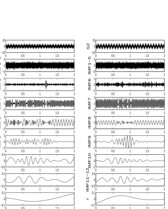
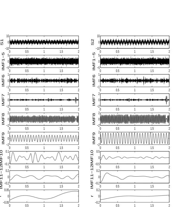
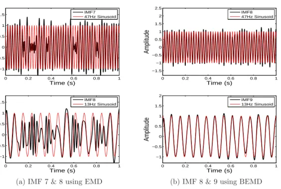
simultaneously. All the IMFs decomposed using EMD and BEMD are shown in Figs. 3.2 and 3.3. In particular, the IMFs containing the two frequency components, 13Hz and 47Hz sinusoids, can be observed in Fig. 3.4. The IMFs decomposed using BEMD contain the sinusoids closer to the original signals with less mode-mixing.

The HHS from the IMFs decomposed using EMD and BEMD are illustrated in Fig. 3.5. Similarly as the raw IMFs, the HHS using BEMD contains more localised time-frequency components across time than EMD, where the time-frequency components around 13Hz and 47Hz in Fig. 3.5 (b) are more prominent than those in Fig. 3.5 (a).

IMF Estimation

In this section, we use the method in [61] and [62] for the performance comparison between EMD and BEMD. The method was designed to enhance the capability of the EMD by utilising linear weights for the IMFs, which were calculated in the minimum mean square error sense. We decomposed the signal x(t) = sf(t) +v(t) using EMD, where sf(t) is a sinusoid of frequency f and v(t) is a realisation of white Gaussian noise (WGN), and subsequently applied the Wiener filter to the IMFs to obtain an estimate of the sinusoid,

(50)

0 0.5 1 1.5 2 −10 0 10 S1 0 0.5 1 1.5 2 −10 0 10 S2 0 0.5 1 1.5 2 −5 0 5 IMF1−5 −5₀ _0.5 ₁ _1.5 ₂ 0 5 IMF1−5 0 0.5 1 1.5 2 −2 0 2 IMF6 0 0.5 1 1.5 2 −1 0 1 IMF6 0 0.5 1 1.5 2 −2 0 2 IMF7 0 0.5 1 1.5 2 −2 0 2 IMF7 0 0.5 1 1.5 2 −2 0 2 IMF8 0 0.5 1 1.5 2 −5 0 5 IMF8 0 0.5 1 1.5 2 −2 0 2 IMF9 0 0.5 1 1.5 2 −2 0 2 IMF9 0 0.5 1 1.5 2 −0.5 0 0.5 IMF10 0 0.5 1 1.5 2 −1 0 1 IMF10 0 0.5 1 1.5 2 −0.2 0 0.2 IMF11−12 0 0.5 1 1.5 2 −0.5 0 0.5 IMF11−12 0 0.5 1 1.5 2 −0.1 0 0.1 r 0 0.5 1 1.5 2 −0.2 0 0.2 r

Figure 3.2: All the decomposed IMFs of the data in eq. (3.1) and (3.2) using EMD.

The left column illustrates the decomposition of x1(t) and right column shows those

(51)

0 0.5 1 1.5 2 −10 0 10 S1 0 0.5 1 1.5 2 −10 0 10 S2 0 0.5 1 1.5 2 −5 0 5 IMF1−5 −5₀ _0.5 ₁ _1.5 ₂ 0 5 IMF1−5 0 0.5 1 1.5 2 −1 0 1 IMF6 0 0.5 1 1.5 2 −1 0 1 IMF6 0 0.5 1 1.5 2 −2 0 2 IMF7 0 0.5 1 1.5 2 −2 0 2 IMF7 0 0.5 1 1.5 2 −2 0 2 IMF8 0 0.5 1 1.5 2 −2 0 2 IMF8 0 0.5 1 1.5 2 −2 0 2 IMF9 0 0.5 1 1.5 2 −2 0 2 IMF9 0 0.5 1 1.5 2 −0.1 0 0.1 IMF10 0 0.5 1 1.5 2 −0.5 0 0.5 IMF10 0 0.5 1 1.5 2 −0.2 0 0.2 IMF11−12 0 0.5 1 1.5 2 −0.2 0 0.2 IMF11−12 0 0.5 1 1.5 2 −0.05 0 0.05 r 0 0.5 1 1.5 2 −0.2 0 0.2 r

Figure 3.3: All the decomposed IMFs of the data in eq. (3.1) and (3.2) using BEMD. The left column illustrates the real parts of the complex IMFs, and the right col-umn shows the imaginary parts of complex IMFs. Note the alleviated mode mixing problems compared to EMD results in Fig. 3.2.

(52)

0 0.2 0.4 0.6 0.8 1 −1 −0.5 0 0.5 1 1.5 Time (s) Amplitude IMF7 47Hz Sinusoid 0 0.2 0.4 0.6 0.8 1 −1.5 −1 −0.5 0 0.5 1 1.5 2 2.5 Time (s) Amplitude IMF8 47Hz Sinusoid 0 0.2 0.4 0.6 0.8 1 −1 −0.5 0 0.5 1 1.5 Time (s) Amplitude IMF8 13Hz Sinusoid 0 0.2 0.4 0.6 0.8 1 −1 −0.5 0 0.5 1 1.5 2 Time (s) Amplitude IMF9 13Hz Sinusoid

(a) IMF 7 & 8 using EMD (b) IMF 8 & 9 using BEMD

Figure 3.4: Comparison between IMFs of EMD and BEMD using the data in eq. (3.1) and (3.2). EMD can decompose the original sinusoids in IMF 7 and IMF 8, and the IMF 8 and IMF 9 of BEMD include those sinusoids. Note that the decomposed IMFs using BEMD are closer to the original sinusoids than those of EMD.

Frequency (Hz) Time (s) 0.2 0.4 0.6 0.8 1 0 10 20 30 40 50 60 70 Frequency (Hz) Time (s) 0.2 0.4 0.6 0.8 1 0 10 20 30 40 50 60 70

(a) HHS using EMD (b) HHS using BEMD

Figure 3.5: HHS of EMD and BEMD for the data in eq. (3.1) and (3.2). Similarly as the results in Fig. 3.4, the HHS of BEMD produces more localised and stable 13Hz and 47Hz frequency components across time.

(53)

ˆ sEMD(t). ˆ sEMD(t) = ˘W T _˘ C (3.3)

where (·)T denotes the vector transpose and ˘C includes all the components of the IMFs and the residue.

˘ C=             c1(1) c1(2) . . . c1(t) c2(1) c2(2) . . . c2(t) .. . ... . .. ... cM(1) cM(2) . . . cM(t) r(1) r(2) . . . r(2)             (3.4) Let D= ˘CC˘T (3.5)

the optimal weight vector ˘W is obtained as

˘

W=D−1_CS_˘ T

f (3.6)

where Sf contains all the values of sf(t). The more accurate the estimate of sf(t), the more accurately the IMFs represent the original input components. Additionally, BEMD was performed onz(t) =sf(t)+vr(t)+j(sf(t)+vi(t)) wherevr(t) andvi(t) denote different realisations of WGN in both the real and imaginary parts of z(t). For comparison with the EMD operation, the Wiener filter was applied to the real part only of the bivariate IMFs to obtain an estimate for the sinusoid, ˆsBEMD(t). This analysis was performed for

several frequencies, and over four signal-to-noise ratio (SNRinit.) levels. The analysis was

also extended tox(t) =fA(sf(t)) +v(t) in the case of EMD andz(t) =fA(sf(t)) +vr(t) + j(fA(sf(t)) +vi(t)) in the case of BEMD where fA(·) denotes an amplitude modulation operation (using 1 or 2Hz sinusoid) to illustrate component estimation for signals with changing amplitudes. The sampling frequency was 256Hz and the signal length 10s.

The average SNR of the reconstructed uniform amplitude sinusoids over 50 simula-tions using EMD and BEMD are given in Table 3.1. The superior performance of BEMD is evident for all considered simulations. Component estimation results for sinusoids

(54)

modu-Algorithm P P P P P P PP SNRinit. Freq. 2Hz 6Hz 12Hz 25Hz 44Hz EMD 5dB 17.2dB 13.3dB 11.1dB 9.0dB 6.5dB BEMD 5dB 18.8dB 13.8dB 11.7dB 9.5dB 7.4dB EMD 0dB 12.6dB 9.7dB 7.5dB 5.5dB 4.1dB BEMD 0dB 14.2dB 10.9dB 9.0dB 6.8dB 5.6dB EMD -5dB 9.2dB 6.0dB 4.3dB 3.0dB 2.2dB BEMD -5dB 10.7dB 7.7dB 5.9dB 4.4dB 3.0dB EMD -10dB 6.3dB 3.5dB 2.3dB 1.3dB 0.9dB BEMD -10dB 7.6dB 4.2dB 3.0dB 2.1dB 1.3dB

Table 3.1: Sinusoid reconstruction (sˆ_EMD(t)andsˆBEMD(t)) results in SNR for different

frequencies and initial noise levels.

Algorithm P P P P P P PP SNRinit. Freq. 2Hz 6Hz 12Hz 25Hz 44Hz EMD 5dB 17.1dB 12.6dB 10.6dB 8.8dB 6.5dB BEMD 5dB 18.1dB 13.8dB 11.6dB 9.5dB 6.9dB EMD 0dB 12.7dB 9.5dB 7.5dB 5.4dB 3.8dB BEMD 0dB 14.1dB 10.3dB 8.1dB 6.1dB 5.1dB EMD -5dB 9.0dB 5.8dB 4.2dB 2.8dB 2.1dB BEMD -5dB 10.0dB 7.5dB 5.9dB 4.3dB 3.0dB EMD -10dB 5.8dB 3.3dB 2.2dB 1.3dB 0.9dB BEMD -10dB 7.0dB 4.3dB 3.0dB 2.1dB 1.3dB

Table 3.2: Reconstruction results of a 1Hz amplitude modulated sinusoid (sˆEMD(t)

and sˆBEMD(t)) in SNR for different frequencies and initial noise levels.

lated at 1Hz and 2Hz are shown respectively in Tables. 3.2 and 3.3. The BEMD algorithm consistently allowed for better component estimation.

For rigour, the simulations were performed over a range of parameters for the stopping criterion, as BEMD and EMD often require different numbers of sifting operations even when using the same stopping criterion. Component estimation performance for the signalsf(t), forf=12Hz and f=44Hz and for 0dB and -10dB SNR, for different numbers of sifting operations (by adjusting the stopping criterion) are shown in Fig. 3.6, where, as before, BEMD consistently outperform EMD. These results illustrate that the enhanced BEMD performance is caused by more accurate component estimation and not by virtue of better sifting.

It can therefore be deduced that the shared information between the real and the imaginary parts of the BEMD allowed for a more accurate estimate of the common

(55)

Algorithm P P P P P P PP SNRinit. Freq. 2Hz 6Hz 12Hz 25Hz 44H