Weakly Supervised Joint Sentiment-Topic
Detection from Text
Chenghua Lin, Yulan He, Richard Everson,
Member,
IEEE, and Stefan Ru¨ger
Abstract—Sentiment analysis or opinion mining aims to use automated tools to detect subjective information such as opinions, attitudes, and feelings expressed in text. This paper proposes a novel probabilistic modeling framework called joint sentiment-topic (JST) model based on latent Dirichlet allocation (LDA), which detects sentiment and topic simultaneously from text. A reparameterized version of the JST model called Reverse-JST, obtained by reversing the sequence of sentiment and topic generation in the modeling process, is also studied. Although JST is equivalent to Reverse-JST without a hierarchical prior, extensive experiments show that when sentiment priors are added, JST performs consistently better than Reverse-JST. Besides, unlike supervised approaches to sentiment classification which often fail to produce satisfactory performance when shifting to other domains, the weakly supervised nature of JST makes it highly portable to other domains. This is verified by the experimental results on data sets from five different domains where the JST model even outperforms existing semi-supervised approaches in some of the data sets despite using no labeled documents. Moreover, the topics and topic sentiment detected by JST are indeed coherent and informative. We hypothesize that the JST model can readily meet the demand of large-scale sentiment analysis from the web in an open-ended fashion. Index Terms—Sentiment analysis, opinion mining, latent Dirichlet allocation (LDA), joint sentiment-topic (JST) model.Ç
1
I
NTRODUCTIONW
ITHthe explosion of Web 2.0, various types of socialmedia such as blogs, discussion forums, and peer-to-peer networks present a wealth of information that can be very helpful in assessing the general public’s sentiment and opinions toward products and services. Recent surveys have revealed that opinion-rich resources like online reviews are having greater economic impact on both consumers and companies compared to the traditional media [1]. Driven by the demand of gleaning insights into such great amounts of user-generated data, work on new methodologies for automated sentiment analysis and discovering hidden knowledge from unstructured text data has bloomed splendidly.
Among various sentiment analysis tasks, one of them is sentiment classification, i.e., identifying whether the se-mantic orientation of the given text is positive, negative, or neutral. Although much work has been done in this line [2], [3], [4], [5], [6], [7], most of the existing approaches rely on supervised learning models trained from labeled corpora where each document has been labeled as positive
or negative prior to training. However, such labeled corpora are not always easily obtained in practical applications. Also, it is well known that sentiment classifiers trained on one domain often fail to produce satisfactory results when shifted to another domain, since sentiment expressions can be quite different in different domains [7], [8]. For example, it is reported in [8] that in-domain Support Vector Machines (SVMs) classifier trained on the movie review (MR) data (giving best accuracy of 90.45 percent) only achieved relatively poor accuracies of 70.29 and 61.36 percent, respectively, when directly tested on book review and product support services data. More-over, aside from the diversity of genres and large-scale size of the web corpora, user-generated content such as online reviews evolves rapidly over time, which demands much more efficient and flexible algorithms for sentiment analysis than the current approaches can offer. These observations have thus motivated the problem of using unsupervised or weakly supervised approaches for do-main-independent sentiment classification.
Another common deficiency of the aforementioned work is that it only focuses on detecting the overall sentiment of a document, without performing an in-depth analysis to discover the latent topics and the associated topic senti-ment. In general, a review can be represented by a mixture of topics. For instance, a standard restaurant review will probably discuss topics or aspects such as food, service, location, price, etc. Although detecting topics is a useful step for retrieving more detailed information, the lack of sentiment analysis on the extracted topics often limits the effectiveness of the mining results, as users are not only interested in the overall sentiment of a review and its topical information, but also the sentiment or opinions toward the topics discovered. For example, a customer may be happy about the food and price, but at the same time be unsatisfied with the service and location. Moreover, it is
. C. Lin is with the Department of Computer Science, College of Engineering, Mathematics and Physical Sciences, University of Exeter, and the Knowledge Media Institute, The Open University, Walton Hall, Milton Keynes MK7 6AA, United Kingdom. E-mail: [email protected].
. Y. He and S. Ru¨ger are with the Knowledge Media Institute, The Open University, Walton Hall, Milton Keynes MK7 6AA, United Kingdom. E-mail: {y.he, s.rueger}@open.ac.uk.
. R. Everson is with the Department of Computer Science, College of Engineering, Mathematics and Physical Sciences, Harrison Building, University of Exeter, Exeter EX4 4QF, United Kingdom.
E-mail: [email protected].
Manuscript received 23 Nov. 2009; revised 5 Sept. 2010; accepted 6 Jan. 2011; published online 7 Feb. 2011.
Recommended for acceptance by X. Zhu.
For information on obtaining reprints of this article, please send e-mail to: [email protected], and reference IEEECS Log Number TKDE-2009-11-0797. Digital Object Identifier no. 10.1109/TKDE.2011.48.
intuitive that sentiment polarities are dependent on topics or domains. A typical example is that when appearing under different topics of the movie review domain, the adjective “complicated” may have negative orientation as “complicated role” in one topic, and conveys positive sentiment as “complicated plot” in another topic. Therefore, detecting topic and sentiment simultaneously should serve a critical function in helping users by providing more informative sentiment-topic mining results.
In this paper, we focus on document-level sentiment classification for general domains in conjunction with topic detection and topic sentiment analysis, based on the proposed weakly supervised joint sentiment-topic (JST) model [9]. This model extends the state-of-the-art topic model latent Dirichlet allocation (LDA) [10], by construct-ing an additional sentiment layer, assumconstruct-ing that topics are generated dependent on sentiment distributions and words are generated conditioned on the sentiment-topic pairs. Our model is distinguished from other sentiment-topic models [11], [12] in that: 1) JST is weakly supervised, where the only supervision comes from a domain independent sentiment lexicon. 2) JST can detect sentiment and topics simultaneously. We suggest that the weakly supervised nature of the JST model makes it highly portable to other domains for the sentiment classification task. While JST is a reasonable design choice for joint sentiment-topic detection, one may argue that the reverse is also true, namely that sentiments may vary according to topics. Thus, we also studied a reparameterized version of JST, called the Reverse-JST model, in which sentiments are generated dependent on topic distributions in the model-ing process. It is worth notmodel-ing that without a hierarchical prior, JST and Reverse-JST are essentially two reparame-terizations of the same model.
Extensive experiments have been conducted with both the JST and Reverse-JST models on the movie review (MR)1 and multidomain sentiment (MDS) data sets.2 Although JST is equivalent to Reverse-JST without hier-archical priors, experimental results show that when sentiment prior information is encoded, these two models exhibit very different behaviors, with JST consistently outperforming Reverse-JST in sentiment classification. The portability of JST in sentiment classification is also verified by the experimental results on the data sets from five different domains, where the JST model even outper-forms existing semi-supervised approaches in some of the data sets despite using no labeled documents. Aside from automatically detecting sentiment from text, JST can also extract meaningful topics with sentiment associations as illustrated by some topic examples extracted from the two experimental data sets.
The rest of the paper is organized as follows. Section 2 introduces related work. Section 3 presents the JST and Reverse-JST models. We describe the experimental setup in Section 4 and discuss the results on the movie review and multidomain sentiment data sets in Section 5. Finally, Section 6 concludes the paper and outlines the future work.
2
R
ELATEDW
ORK2.1 Sentiment Classification
Machine learning techniques have been widely deployed for sentiment classification at various levels, e.g., from the document level, to the sentence and word/phrase level. On the document level, one tries to classify documents as positive, negative, or neutral, based on the overall sentiments expressed by opinion holders. There are several lines of representative work at the early stage [2], [3]. Turney [2] used weakly supervised learning with mutual information to predict the overall document sentiment by averaging out the sentiment orientation of phrases within a document. Pang et al. [3] classified the polarity of movie reviews with the traditional supervised machine learning approaches and achieved the best results using SVMs. In their subsequent work [4], the sentiment classification accuracy was further improved by employing a subjectiv-ity detector and performing classification only on the subjective portions of reviews. The annotated movie review data set (also known as polarity data set) used in [3] and [4] has later become a benchmark for many studies [5], [6]. Whitelaw et al. [5] used SVMs to train on combinations of different types of appraisal group features and bag-of-words features, whereas Kennedy and Inkpen [6] leveraged two main sources, i.e., General Inquirer and Choose the Right Word [13], and trained two different classifiers for the sentiment classification task.
As opposed to the work [2], [3], [4], [5], [6] that only focused on sentiment classification in one particular domain, some researchers have addressed the problem of sentiment classification across domains [7], [8]. Aue and Gamon [8] explored various strategies for customizing sentiment classifiers to new domains, where training is based on a small number of labeled examples and large amounts of unlabeled in-domain data. It was found that directly applying a classifier trained on a particular domain barely outperforms the baseline for another domain. In the same vein, more recent work [7], [14] focused on domain adaptation for sentiment classifiers. Blitzer et al. [7] addressed the domain transfer problem for sentiment classification using the structural correspondence learning (SCL) algorithm, where the frequent words in both source and target domains were first selected as candidate pivot features and pivots were then chosen based on the mutual information between these candidate features and the source labels. They achieved an overall improvement of 46 percent over a baseline model without adaptation. Li and Zong [14] combined multiple single classifiers trained on individual domains using SVMs. However, their approach relies on labeled data from all domains to train an integrated classifier and thus may lack flexibility to adapt the trained classifier to other domains where no label information is available.
All the aforementioned work shares some similar limita-tions: 1) they focused on sentiment classification alone without considering the mixture of topics in the text, which limits the effectiveness of the mining results to users. 2) Most of the approaches [3], [4], [7], [15] favor supervised learning, requiring labeled corpora for training, and potentially limiting the applicability to other domains of interest.
1. http://www.cs.cornell.edu/people/pabo/movie-review-data. 2. http://www.cs.jhu.edu/~mdredze/datasets/sentiment/index2.html.
Compared to the traditional topic-based text classifica-tion, sentiment classification is deemed to be more challen-ging as sentiment is often embodied in subtle linguistic mechanisms such as the use of sarcasm or incorporated with highly domain-specific information. Among various efforts for improving sentiment detection accuracy, one of the directions is to incorporate prior information from the general sentiment lexicon (i.e., words bearing positive or negative sentiment) into sentiment models. These general lists of sentiment lexicons can be acquired from domain-independent sources in many different ways, i.e., from manually built appraisal groups [5], to semiautomatically [16] or fully automatically [17] constructed lexicons. When incorporating lexical knowledge as prior information into a sentiment-topic model, Andreevskaia and Bergler [18] integrated the lexicon-based and corpus-based approaches for sentence-level sentiment annotation across different domains. A recently proposed nonnegative matrix tri-factorization approach [19] also employed lexical prior knowledge for semi-supervised sentiment classification, where the domain-independent prior knowledge was incorporated in conjunction with domain-dependent un-labeled data and a few un-labeled documents. However, this approach performed worse than the JST model on the movie review data even with 40 percent labeled documents, as will be discussed in Section 5.
2.2 Sentiment-Topic Models
JST models sentiment and mixture of topics simultaneously. Although work in this line is still relatively sparse, some studies have preserved a similar vision [11], [12], [20]. Most closely related to our work is the Topic-Sentiment Model (TSM) [11], which models mixture of topics and sentiment predictions for the entire document. However, there are several intrinsic differences between JST and TSM. First, TSM is essentially based on the probabilistic latent semantic indexing (pLSI) [21] model with an extra background component and two additional sentiment subtopics, whereas JST is based on LDA. Second, regarding topic extraction, TSM samples a word from the background component model if the word is a common English word. Otherwise, a word is sampled from either a topical model or one of the sentiment models (i.e., positive or negative sentiment model). Thus, in TSM the word generation for positive or negative sentiment is not conditioned on topic.
This is a crucial difference compared to the JST model as in JST one draws a word from the distribution over words jointly conditioned on both topic and sentiment label. Third, for sentiment detection, TSM requires postprocessing to calculate the sentiment coverage of a document, while in JST the document sentiment can be directly obtained from the probability distribution of sentiment label given a document. Other models by Titov and McDonald [12], [20] are also closely related to ours, since they are all based on LDA. The Multi-Grain Latent Dirichlet Allocation model (MG-LDA) [20] is argued to be more appropriate to build topics that are representative of ratable aspects of customer reviews, by allowing terms being generated from either a global topic or a local topic. Being aware of the limitation that MG-LDA is still purely topic-based without considering the associations between topics and sentiments, Titov and McDonald further proposed the Multi-Aspect Sentiment model (MAS) [12] by extending the MG-LDA framework. The major improvement of MAS is that it can aggregate sentiment text for the sentiment summary of each rating aspect extracted from MG-LDA. Our model differs from MAS in several aspects. First, MAS works in a supervised setting as it requires that every aspect is rated at least in some documents, which is infeasible in real-world applica-tions. In contrast, JST is weakly supervised with only minimum prior information being incorporated, which in turn is more flexible. Second, the MAS model was designed for sentiment text extraction or aggregation, whereas JST is more suitable for the sentiment classification task.
3
M
ETHODOLOGY3.1 Joint Sentiment-Topic Model
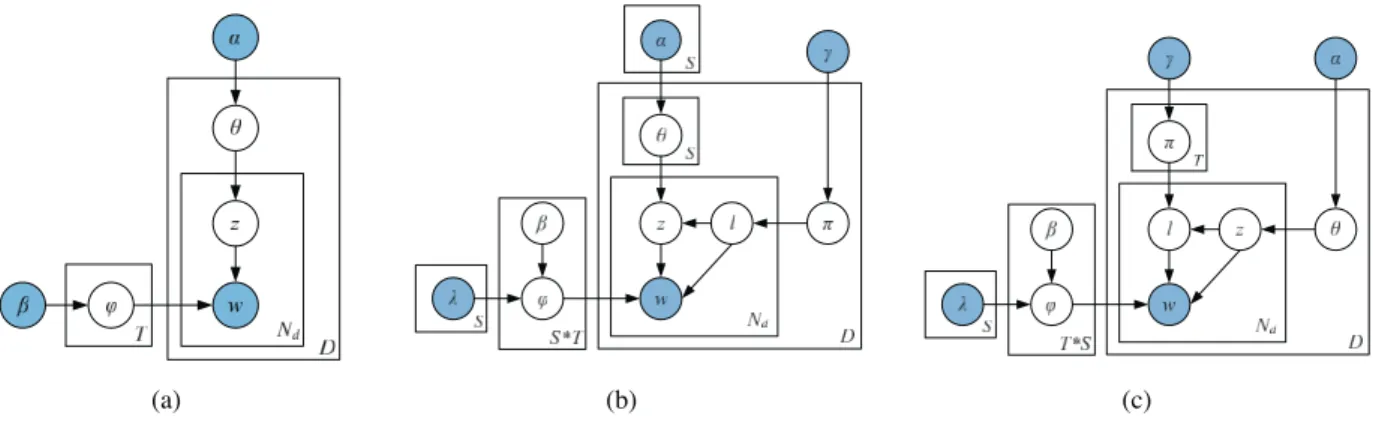
The LDA model, as shown in Fig. 1a, is based upon the assumption that documents are mixture of topics, where a topic is a probability distribution over words [10], [22]. Generally, the procedure for generating a word in a document under LDA can be broken down into two stages. One first chooses a distribution over a mixture ofTtopics for the document. Following that, one picks a topic randomly from the topic distribution, and draws a word from that topic according to the corresponding topic-word distribution.
The existing framework of LDA has three hierarchical layers, where topics are associated with documents, and words are associated with topics. In order to model
document sentiments, we propose a joint sentiment-topic model [9] by adding an additional sentiment layer between the document and the topic layers. Hence, JST is effectively a four-layer model, where sentiment labels are associated with documents, under which topics are associated with sentiment labels and words are associated with both sentiment labels and topics. A graphical model of JST is represented in Fig. 1b.
Assume that we have a corpus with a collection of D documents denoted byC¼ fd1; d2;. . .; dDg; each document
in the corpus is a sequence of Nd words denoted by
d¼ ðw1; w2;. . .; wNdÞ, and each word in the document is an item from a vocabulary index withV distinct terms denoted by f1;2;. . .; Vg. Also, let S be the number of distinct sentiment labels, and T be the total number of topics. The procedure for generating a word wi in document d under
JST boils down to three stages. First, one chooses a sentiment label l from the per-document sentiment dis-tribution d. Following that, one chooses a topic from the
topic distribution d;l, where d;l is conditioned on the
sampled sentiment labell. It is worth noting that the topic distribution of JST is different from that of LDA. In LDA, there is only one topic distribution for each individual document. In contrast, in JST each document is associated withS(the number of sentiment labels) topic distributions, each of which corresponds to a sentiment label l with the same number of topics. This feature essentially provides means for the JST model to predict the sentiment associated with the extracted topics. Finally, one draws a word from the per-corpus word distribution conditioned on both topic and sentiment label. This is again different from LDA that in LDA a word is sampled from the word distribution only conditioned on topic.
The formal definition of the generative process in JST corresponding to the graphical model shown in Fig. 1b is as follows:
. For each sentiment labell2 f1;. . .; Sg
- For each topic j2 f1;. . .; Tg, draw ’lj
DirðlTljÞ.
. For each document d, choose a distribution d
DirðÞ.
. For each sentiment labellunder documentd, choose a distributiond;lDirðÞ.
. For each wordwi in documentd
- choose a sentiment labelliMultðdÞ, - choose a topicziMultðd;liÞ,
- choose a word wi from ’lizi, a multinomial distribution over words conditioned on topiczi
and sentiment labelli.
The hyperparametersandin JST can be treated as the prior observation counts for the number of times topic j associated with sentiment label l is sampled from a document and the number of times words sampled from topic jare associated with sentiment label l, respectively, before having observed any actual words. Similarly, the hyperparametercan be interpreted as the prior observation counts for the number of times sentiment label l sampled from a document before any word from the corpus is observed. In our implementation, we used asymmetric prior
and symmetric priorand. In addition, there are three sets of latent variables that we need to infer in JST, i.e., the per-document sentiment distribution , the per-document sentiment label specific topic distribution , and the per-corpus joint sentiment-topic word distribution’. We will see later in the paper that the per-document sentiment distribu-tionplays an important role in determining the document sentiment polarity.
3.1.1 Incorporating Model Priors
We modified Phan’s Gibbs LDAþþ package3 for the implementation of JST and Reverse-JST. Compared to the original LDA model, besides adding a sentiment label generation layer, we also added an additional dependency link of’ on the matrix of sizeSV, which we used to encode word prior sentiment information into the JST and Reverse-JST models. The matrix can be considered as a transformation matrix which modifies the Dirichlet priors of sizeSTV, so that the word prior sentiment polarity can be captured.
The complete procedure of incorporating prior knowl-edge into the JST model is as follows: first, is initialized with all the elements taking a value of 1. Then, for each term w2 f1;. . .; Vg in the corpus vocabulary and for each sentiment labell2 f1;. . .; Sg, ifwis found in the sentiment lexicon, the elementlwis updated as follows:
lw¼
1; ifSðwÞ ¼l;
0; otherwise;
ð1Þ where the functionSðwÞreturns the prior sentiment label of win a sentiment lexicon, i.e., neutral, positive, or negative. For example, the word “excellent” with index i in the vocabulary has a positive sentiment polarity. The corre-sponding row vector in is ½0;1;0 with its elements representing neutral, positive, and negative prior polarity. For each topicj2 f1;. . .; Tg, multiplyingli withlji, only
the value oflposjiis retained, andlneujiandlnegjiare set to 0. Thus, “excellent” can only be drawn from the positive topic word distributions generated from a Dirichlet distribution with parameterlpos.
The previously proposed DiscLDA [23] and Labeled LDA [24] also utilize a transformation matrix to modify Dirichlet priors by assuming the availability of document class labels. DiscLDA uses a class-dependent linear transformation to project a K-dimensional (K latent topics) document-topic distribution into aL-dimensional space (Ldocument labels), while Labeled LDA simply defines a one-to-one correspon-dence between LDA’s latent topics and document labels. In contrast to this work, we use word prior sentiment as supervised information and modify the topic-word Dirichlet priors for sentiment classification.
3.1.2 Model Inference
In order to obtain the distributions of,, and ’, we first estimate the posterior distribution over z and l, i.e., the assignment of word tokens to topics and sentiment labels. The sampling distribution for a word given the remaining topics and sentiment labels is Pðzt¼j; lt¼kjw;zt;lt;
; ; Þ, where zt and lt are vectors of assignments of
topics and sentiment labels for all the words in the collection except for the word at positiontin documentd. The joint probability of the words, topics, and senti-ment label assignsenti-ments can be factored into the following three terms:
Pðw;z;lÞ ¼Pðwjz;lÞPðz;lÞ ¼Pðwjz;lÞPðzjlÞPðlÞ: ð2Þ For the first term, by integrating out’, we obtain
Pðwjz;lÞ ¼ ðV Þ ðÞV !ST Y k Y j Q iðNk;j;iþÞ ðNk;jþV Þ ; ð3Þ whereNk;j;iis the number of times wordiappeared in topic
j and with sentiment label k,Nk;j is the number of times
words are assigned to topicjand sentiment labelk, andis the gamma function.
For the second term, by integrating out, we obtain
PðzjlÞ ¼ PT j¼1k;j QT j¼1ðk;jÞ !DS Y d Y k Q jðNd;k;jþk;jÞ ðNd;kþPjk;jÞ ; ð4Þ whereDis the total number of documents in the collection,
Nd;k;jis the number of times a word from documentdbeing
associated with topicjand sentiment labelk, andNd;kis the
number of times sentiment labelkbeing assigned to some word tokens in documentd.
For the third term, by integrating out, we obtain
PðlÞ ¼ ðSÞ ðÞS !D Y d Q kðNd;kþÞ ðNdþSÞ ; ð5Þ whereNdis the total number of words in documentd.
Gibbs sampling was used to estimate the posterior distribution by sampling the variables of interest, ztand lt
here, from the distribution over the variables given the current values of all other variables and data. Letting the superscripttdenote a quantity that excludes data fromtth position, the conditional posterior for zt andlt by
margin-alizing out the random variables’,, andis Pðzt¼j; lt¼kjw;zt;lt; ; ; Þ /N t k;j;wtþ Nt k;jþV N t d;k;jþk;j Nt d;kþ P jk;j N t d;kþ Nt d þS : ð6Þ Samples obtained from the Markov chain are then used to approximate the per-corpus sentiment-topic word distribution
’k;j;i¼
Nk;j;iþ
Nk;jþV
: ð7Þ
The approximate per-document sentiment label specific topic distribution is
d;k;j¼
Nd;k;jþk;j
Nd;kþPjk;j
: ð8Þ
Finally, the approximate per-document sentiment dis-tribution is
d;k¼
Nd;kþ
NdþS
: ð9Þ
The pseudocode for the Gibbs sampling procedure of JST is shown in Algorithm 1.
Algorithm 1.Gibbs sampling procedure of JST. Require:; ; , Corpus
Ensure:sentiment and topic label assignment for all word tokens in the corpus
1: InitializeSTV matrix; DST matrix, DSmatrix.
2: fori¼1tomaxGibbs sampling iterationsdo 3: forall documentsd2 ½1; Mdo
4: forall wordst2 ½1; Nddo
5: Exclude wordtassociated with sentiment label land topic labelzfrom variablesNk;j;i; Nk;j,
Nd;k;j; Nd;k, and Nd;
6: Sample a new sentiment-topic pairl~andz~using Equation 6;
7: Update variablesNk;j;i; Nk;j,Nd;k;j,Nd;k, andNd
using the new sentiment label~land topic labelz;~
8: end for 9: end for
10: forevery 25 iterationsdo
11: Update hyperparameterwith the maximum-likelihood estimation; 12: end for
13: forevery 100 iterationsdo
14: Update the matrix,, andwith new sampling results;
15: end for 16: end for
3.2 Reverse Joint Sentiment-Topic (Reserve-JST) Model
In this section, we study a reparameterized version of the JST model called Reverse-JST. As opposed to JST in which topic generation is conditioned on sentiment labels, senti-ment label generation in Reverse-JST is dependent on topics. As shown in Fig. 1c, the Reverse-JST model is a four-layer hierarchical Bayesian model, where topics are associated with documents, under which sentiment labels are associated with topics and words are associated with both topics and sentiment labels. Using similar notations and terminologies as in Section 3.1, the joint probability of the words, the topics and sentiment label assignments of Reverse-JST can be factored into the following three terms: Pðw;l;zÞ ¼Pðwjl;zÞPðl;zÞ ¼Pðwjl;zÞPðljzÞPðzÞ: ð10Þ It is easy to derive the Gibbs sampling for Reverse-JST in the same way as JST. Therefore, here we only give the full conditional posterior forztandltby marginalizing out the
random variables’,, and
Pðzt¼j; lt¼kjw;zt;lt; ; ; Þ /N t j;k;wtþ Nt j;kþV N t d;j;kþ Nt d;jþS N t d;jþj Nt d þ P jj : ð11Þ As we do not have a direct per-document sentiment distribution in Reverse-JST, a distribution over sentiment labels for documentPðljdÞis calculated based on the topic
specific sentiment distribution and the per-document topic proportion PðljdÞ ¼X z Pðljz; dÞPðzjdÞ: ð12Þ
4
E
XPERIMENTALS
ETUP4.1 Data Sets Description
Two publicly available data sets, the MR and MDS data sets, were used in our experiments. The MR data set has become a benchmark for many studies since the work of Pang et al. [3]. The version 2.0 used in our experiment consists of 1,000 positive and 1,000 negative movie reviews crawled from the IMDB movie archive, with an average of 30 sentences in each document. We also experimented with another data set, namely subjective MR, by removing the sentences that do not bear opinion information from the MR data set, following the approach of Pang and Lee [4]. The resulting data set still contains 2,000 documents with a total of 334,336 words and 18,013 distinct terms, about half the size of the original MR data set without performing subjectivity detection.
First used by Blitzer et al. [7], the MDS data set contains four different types of product reviews crawled from Amazon.com including Book, DVD, Electronics, and Kitchen, with 1,000 positive and 1,000 negative examples for each domain.4
Preprocessing was performed on both of the data sets. First, punctuation, numbers, nonalphabet characters and stop words were removed. Second, standard stemming was performed in order to reduce the vocabulary size and address the issue of data sparseness. Summary statistics of
the data sets before and after preprocessing are shown in Table 1.
4.2 Defining Model Priors
In the experiments, two subjectivity lexicons, namely the MPQA5 and the appraisal lexicons,6 were combined and
incorporated as prior information into the model learning. These two lexicons contain lexical words whose polarity orientation have been fully specified. We extracted the words with strong positive and negative orientation and performed stemming in the preprocessing. In addition, words whose polarity changed after stemming were removed automatically, resulting in 1,584 positive and 2,612 negative words, respectively. It is worth noting that the lexicons used here are fully domain independent and do not bear any supervised information specifically to the MR, subjMR, and MDS data sets. Finally, the prior information was produced by retaining all words in the MPQA and appraisal lexicons that occurred in the experimental data sets. Statistics about the prior information for each data set are listed in Table 2. It can be observed that the prior positive words occur much more frequently than the negative words, with frequencies at least doubling those of negative words in all of the data sets.
4.3 Hyperparameter Settings
Previous study has shown that while LDA can produce reasonable results with a simple symmetric Dirichlet prior, an asymmetric prior over the document-topic distributions has substantial advantage over a symmetric prior [25]. In the JST model implementation, we set the symmetric prior¼0:01
[22], the symmetric prior ¼ ð0:05LÞ=S, where Lis the average document length,Sthe is total number of sentiment
TABLE 1 Data Set Statistics
Note:ydenotes before preprocessing and * denotes after preprocessing. TABLE 2
Prior Information Statistics
4. We did not perform subjectivity detection on the MDS data set since its average document length is much shorter than that of the MR data set, with some documents even containing only a single sentence.
5. http://www.cs.pitt.edu/mpqa/.
labels, and the value of 0.05 on average allocates 5 percent of probability mass for mixing. The asymmetric prior is learned directly from data using maximum-likelihood estimation [26] and updated every 25 iterations during the Gibbs sampling procedure. In terms of Reverse-JST, we set the symmetric ¼0:01, ¼ ð0:05LÞ=ðTSÞ, and the asymmetric prioris also learned from data as in JST. 4.4 Classifying Document Sentiment
The document sentiment is classified based on PðljdÞ, the probability of a sentiment label given document. In our experiments, we only consider the probability of positive and negative labels for a given document, with the neutral label probability being ignored. There are two reasons for this. First, sentiment classification for both the MR and MDS data sets is effectively a binary classification problem, i.e., documents are being classified either as positive or negative, without the alternative of neutral. Second, the prior information we incorporated merely contributes to the positive and negative words, and consequently there will be much more influence on the probability distribution of positive and negative labels for a given document, rather than the distribution of neutral labels in the given document. Therefore, we define that a document d is classified as a positive-sentiment document if the probability of a positive sentiment label PðlposjdÞ is greater than its probability of
negative sentiment labelPðlnegjdÞ, and vice versa.
5
E
XPERIMENTALR
ESULTSIn this section, we present and discuss the experimental results of both document-level sentiment classification and topic extraction, based on the MR and MDS data sets. 5.1 Sentiment Classification Results versus
Different Number of Topics
As both JST and Reverse-JST model sentiment and topic mixtures simultaneously, it is therefore worth exploring how the sentiment classification and topic extraction tasks affect/benefit each other and in addition, how these two models behave with different topic number settings on different data sets when prior information is incorporated. With this in mind, we conducted a set of experiments on JST and Reverse-JST, with topic number T 2 f1;5;10;15;20;
25;30g. It is worth noting that as JST models the same number of topics under each sentiment label, with three sentiment labels, the total topic number of JST will be equivalent to a standard LDA model with T 2 f3;15;30;
45;60;75;90g.
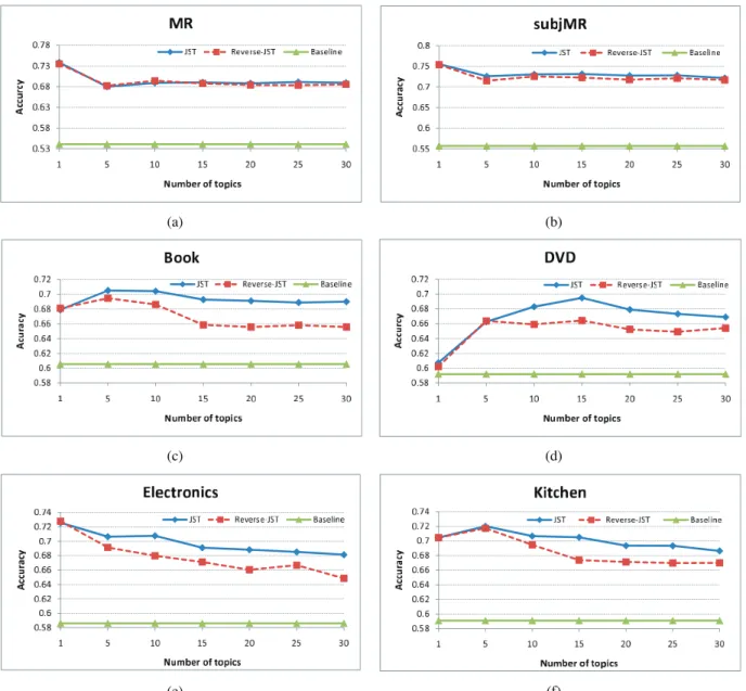
Fig. 2 shows the sentiment classification results of both JST and Reverse-JST at document level with prior informa-tion extracted from the MPQA and appraisal lexicons. For all the reported results, accuracy is used as performance measure and the results were averaged over 10 runs. The baseline is calculated by counting the overlap of the prior lexicon with the training corpus. If the positive sentiment word count is greater than that of the negative words, a document is classified as positive, and vice versa. The improvement over this baseline will reflect how much JST and Reverse-JST can learn from data.
As can be seen from Fig. 2, both JST and Reverse-JST have a significant improvement over the baseline in all of the data sets. When the topic number is set to 1, both JST and Reverse-JST essentially become the standard LDA model with only three sentiment topics, and hence ignore the correlation between sentiment labels and topics. Figs. 2c, 2d, and 2f show that both JST and Reverse-JST perform better with multiple topic settings in the Book, DVD, and Kitchen domains; especially noticeable is JST with 10 percent improvement at T¼15 over single topic setting on the DVD domain. This observation shows that modeling sentiment and topics simultaneously dose indeed help improve sentiment classification. For the cases where a single topic performs the best (i.e., Figs. 2a, 2b, and 2e), it is observed that apart from the MR data set, the drop in sentiment classification accuracy by additionally modeling mixtures of topics is only marginal (i.e., 1 and 2 percent point drop in subjMR and Electronics, respectively), but both JST and Reverse-JST are able to extract sentiment-oriented topics in addition to document-level sentiment detection.
When comparing JST with Reverse-JST, there are three observations. First, JST outperforms Reverse-JST in most of the data sets with multiple topic settings, with up to 4 percent difference in the Book domain. Second, the performance difference between JST and Reverse-JST has some correlation with the corpus size (cf. Table 1). That is, when the corpus size is large these two models perform almost the same, e.g., on the MR data set. In contrast, when the corpus size is relatively small JST significantly outper-forms Reverse-JST, e.g., on the MDS data set. A significance measure based on the paired t-Test (critical P¼0:05) is reported in Table 3. Third, for both models, the sentiment classification accuracy is less affected by topic number settings when the data set size is large. For instance, classification accuracy stays almost the same for the MR and subjMR data sets when topic number is increased from 5 to 30, whereas in contrast, a 2-3 percent drop is observed for Electronics and Kitchen. By closely examining the posterior of JST and Reverse-JST (cf. (6) and (11)), we noticed that the countNd;j(number of times topicjis associated with some
word tokens in document d) in the Reverse-JST posterior would be relatively small due to the factor of a large topic number setting. On the contrary, the countNd;k(number of
times sentiment labelkis assigned to some word tokens in documentd) in the JST posterior would be relatively large as k is only defined over three different sentiment labels. This essentially makes JST less sensitive to the data sparseness problem and to the perturbation of hyperpara-meter settings. In addition, JST encodes the assumption that there is approximately a single sentiment for the entire document, i.e., documents are mostly either positive or negative. This assumption is important as it allows the model to cluster different terms which share similar sentiment. In Reverse-JST, this assumption is not enforced unless only one topic for each sentiment label is defined. Therefore, JST appears to be a more appropriate model design for joint sentiment-topic detection.
5.2 Comparison with Existing Models
In this section, we compare the overall sentiment classification performance of JST and Reverse-JST with
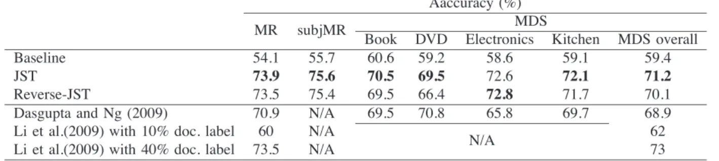
some existing semi-supervised approaches [19], [27]. As can be seen from Table 4, the baseline results calculated based on the sentiment lexicon are below 60 percent for most of the data sets. By incorporating the same prior lexicon, a significant improvement is observed for JST and Reverse-JST over the baseline, where both models have
over 20 percent performance gain on the MR and subjMR data sets, and 10-14 percent improvement on the MDS data set. For the movie review data, there is a further 2 percent improvement for both models on the subjMR data set over the original MR data set. This suggests that though the subjMR data set is in a much compressed form, it is more effective than the full data set as it retains comparable polarity information in a much cleaner way [4]. In terms of the MDS data set, both JST and Reverse-JST perform better on Electronics and Kitchen than Book and DVD, with about 2 percent difference in accuracy. Manually analyzing the MDS data set reveals that the Book and DVD reviews often contain a lot of descriptions of book contents or movie plots, which makes the reviews of these two domains difficult to classify; in contrast, in Electronics and Kitchen domains, comments on products are often expressed in a much more straightforward manner. In terms of the overall performance, except in Electronics, it was observed that JST performed slightly better than Reverse-JST in all sets of experiments, with differences of 0.2 to 3 percent being observed.
Fig. 2. Sentiment classification accuracy versus different topic number settings.
TABLE 3 Significant Test Results
Note: blank denotes the performance of JST and Reverse-JST is significantly undistinguishable; * denotes JST significantly outperforms Reverse-JST.
When compared to the recently proposed weakly supervised approach based on a spectral clustering algo-rithm [27], except in the DVD domain where its accuracy is slightly lower, JST achieved better performance with more than 3 percent overall improvement. We point out that the proposed approach [27] requires users to specify which dimensions (defined by the eigenvectors in spectral cluster-ing) are most closely related to sentiment by inspecting a set of features derived from the reviews for each dimension, and clustering is performed again on the data to derive the final results. In contrast, for the JST and Reverse-JST models proposed here, no human judgement is required. Another recently proposed nonnegative matrix tri-factorization approach [19] also employed lexical prior knowledge for semi-supervised sentiment classification. However, when incorporating 10 percent of labeled documents for training, the nonnegative matrix tri-factorization approach per-formed much worse than JST, with only around 60 percent accuracy being achieved for all the data sets. Even with 40 percent labeled documents, it still performs worse than JST on the MR data set and only slightly outperforms JST on the MDS data set. It is worth noting that no labeled documents were used in the JST results reported here.
5.3 Sentiment Classification Results with Different Features
While JST and Reverse-JST models can give better or comparable performance in document-level sentiment clas-sification compared to semi-supervised approaches [19], [27] with unigram features, it is worth considering the depen-dency between words since it might serve an important function in sentiment analysis. For instance, phrases expressing negative sentiment such as “not good” or “not durable” will convey completely different polarity meanings without considering negations. Therefore, we extended the JST and Reverse-JST models to include higher order information, i.e., bigrams, for model learning. Table 5 shows
the feature statistics of the data sets in unigrams, bigrams, and the combination of both. For the negator lexicon, we collect a handful of words from the General Inquirer under the NOTLWcategory.7We experimented with topic number T 2 f1;5;10;15;20;25;30g. However, it was found that JST and Reverse-JST achieved best results with single topic on bigrams and the combination of bigrams and unigrams most of the time, except for a few cases where multiple topics performed better (i.e., JST and Reverse-JST with T ¼5on Book using unigramsþbigrams, as well as Reverse-JST with T ¼10 on Electronics using unigramsþ bigrams). This is probably due to the fact that bigram features have much lower frequency counts than unigrams. Thus, with the sparse feature cooccurrence, multiple topic settings likely fail to cluster different terms that share similar sentiment and hence harm the sentiment classification accuracy.
Table 6 shows the sentiment classification results of JST and Reverse-JST using different features. It can be observed that both JST and Reverse-JST perform almost the same with unigrams or bigrams on the MR, subjMR, and Book data sets. However, using bigrams gives a better accuracy in DVD but is worse on Electronics and Kitchen compared to using unigrams for both models. When combining both unigrams and bigrams, a performance gain is observed for most of the data sets except the Kitchen data. For both MR and subjMR, using the combination of unigrams and bigrams gives more than 2 percent improvement compared to using either unigrams or bigrams alone, with 76.6 and 77.7 percent accuracy being achieved on these two data sets, respectively. For the MDS data set, the combined features slightly outperform unigrams and bigrams on Book and gives a significant gain on DVD (i.e., 3 percent over unigrams; 1.2 percent over bigrams) and Electronics (i.e., 2.3 percent over unigrams; 4.7 percent over bigrams). Thus,
TABLE 4
Performance Comparison with Existing Models
Note: Boldface denotes the best results.
TABLE 5
Unigram and Bigram Features Statistics
we may conclude that the combination of unigrams and bigrams gives the best overall performance.
5.4 Topic Extraction
The second goal of JST is to extract topics from the MR (without subjectivity detection) and MDS data sets, and evaluate the effectiveness of topic sentiment captured by the model. Unlike the LDA model where a word is drawn from the topic-word distribution, in JST one draws a word from the per-corpus word distribution conditioned on both topics and sentiment labels. Therefore, we analyze the extracted topics under positive and negative sentiment label, separately.
Twenty topic examples extracted from the MR and MDS data sets are shown in Table 7, where each topic was drawn from a particular domain under a sentiment label.
Topics on the top half of Table 7 were generated under the positive sentiment label and the remaining topics were generated under the negative sentiment label, each of which is represented by the top 15 topic words. As can be seen from the table that the extracted topics are quite informative and coherent. The movie review topics try to capture the underlying theme of a movie or the relevant comments from a movie reviewer, while the topics from the MDS data set represent a certain product review from
TABLE 6
Sentiment Classification Results with Different Features
Note: Boldface denotes the best results.
TABLE 7
the corresponding domain. For example, for the two positive sentiment topics under the movie review domain, the first is closely related to the very popular romantic movie “Titanic” directed by James Cameron and starring by Leonardo DiCaprio and Kate Winslet, whereas the other one is likely to be a positive review for a movie. Regarding the MDS data set, the first topics for Book and DVD under the positive sentiment label probably discuss a good cookbook and a popular action movie by Jackie Chan, respectively; for the first negative topic of Electro-nics, it is likely to be about complaints regarding data loss due to the flash drive failure, while the first negative topic of the kitchen domain is probably the dissatisfaction with the high noise level of the Vornado brand fan.
In terms of topic sentiment, by examining each of the topics in Table 7, it is quite evident that most of the positive and negative topics indeed bear positive and negative sentiment. The first movie review topic and the second Book topic under the positive sentiment label mainly describe movie plot and the contents of a book, with fewer words carrying positive sentiment compared to other positive sentiment topics under the same domain. Manually examin-ing the data reveals that the terms that seem not convey sentiments under the topic in fact appear in the context of expressing positive sentiments. Overall, the above analysis illustrates the effectiveness of JST in extracting opinionated topics from a corpus.
6
C
ONCLUSIONS ANDF
UTUREW
ORKIn this paper, we presented a joint sentiment-topic model and a reparameterized version of JST called Reverse-JST. While most of the existing approaches to sentiment classification favor supervised learning, both JST and Reverse-JST models target sentiment and topic detection simultaneously in a weakly supervised fashion. Without a hierarchical prior, JST and Reverse-JST are essentially equivalent. However, extensive experiments conducted on data sets across different domains reveal that these two models behave very differently when sentiment prior knowledge is incorporated, in which case JST consistently outperformed Reverse-JST. For general domain sentiment classification, by incorporating a small amount of domain-independent prior knowledge, the JST model achieved either better or comparable performance compared to existing semi-supervised approaches despite using no labeled documents, which demonstrates the flexibility of JST in the sentiment classification task. Moreover, the topics and topic sentiments detected by JST are indeed coherent and informative.
There are several directions we plan to investigate in the future. One is incremental learning of the JST parameters when facing with new data. Another one is the modifica-tion of the JST model with other supervised informamodifica-tion being incorporated into JST model learning, such as some known topic knowledge for certain product reviews or document labels derived automatically from the user supplied review ratings.
R
EFERENCES[1] B. Pang and L. Lee, “Opinion Mining and Sentiment Analysis,”
J. Foundations and Trends in Information Retrieval,vol. 2, nos. 1/2, pp. 1-135, 2008.
[2] P.D. Turney, “Thumbs Up Or Thumbs Down?: Semantic Orienta-tion Applied to Unsupervised ClassificaOrienta-tion of Reviews,”Proc. Assoc. for Computational Linguistics (ACL ’01),pp. 417-424, 2001.
[3] B. Pang, L. Lee, and S. Vaithyanathan, “Thumbs Up?: Sentiment Classification Using Machine Learning Techniques,” Proc. ACL Conf. Empirical Methods in Natural Language Processing (EMNLP),
pp. 79-86, 2002.
[4] B. Pang and L. Lee, “A Sentimental Education: Sentiment Analysis Using Subjectivity Summarization Based on Minimum Cuts,”
Proc. 42th Ann. Meeting on Assoc. for Computational Linguistics (ACL),pp. 271-278, 2004.
[5] C. Whitelaw, N. Garg, and S. Argamon, “Using Appraisal Groups for Sentiment Analysis,”Proc. 14th ACM Int’l Conf. Information and Knowledge Management (CIKM),pp. 625-631, 2005.
[6] A. Kennedy and D. Inkpen, “Sentiment Classification of Movie Reviews Using Contextual Valence Shifters,” Computational Intelligence,vol. 22, no. 2, pp. 110-125, 2006.
[7] J. Blitzer, M. Dredze, and F. Pereira, “Biographies, Bollywood, Boom-Boxes and Blenders: Domain Adaptation for Sentiment Classification,” Proc. Assoc. for Computational Linguistics (ACL),
pp. 440-447, 2007.
[8] A. Aue and M. Gamon, “Customizing Sentiment Classifiers to New Domains: A Case Study,”Proc. Recent Advances in Natural Language Processing (RANLP),2005.
[9] C. Lin and Y. He, “Joint Sentiment/Topic Model for Sentiment Analysis,” Proc. 18th ACM Conf. Information and Knowledge Management (CIKM),pp. 375-384, 2009.
[10] D.M. Blei, A.Y. Ng, and M.I. Jordan, “Latent Dirichlet Allocation,”
J. Machine Learning Research,vol. 3, pp. 993-1022, 2003.
[11] Q. Mei, X. Ling, M. Wondra, H. Su, and C. Zhai, “Topic Sentiment Mixture: Modeling Facets and Opinions in Weblogs,”Proc. 16th Int’l Conf. World Wide Web (WWW),pp. 171-180, 2007.
[12] I. Titov and R. McDonald, “A Joint Model of Text and Aspect Ratings for Sentiment Summarization,”Proc. Assoc. Computational Linguistics—Human Language Technology (ACL-HLT),pp. 308-316, 2008.
[13] S. Hayakawa and E. Ehrlich, Choose the Right Word: A Con-temporary Guide to Selecting the Precise Word for Every Situation.
HarperPerennial, 1994.
[14] S. Li and C. Zong, “Multi-Domain Sentiment Classification,”Proc. Assoc. Computational Linguistics—Human Language Technology (ACL-HLT),pp. 257-260, 2008.
[15] R. McDonald, K. Hannan, T. Neylon, M. Wells, and J. Reynar, “Structured Models for Fine-to-Coarse Sentiment Analysis,”Proc. Assoc. for Computational Linguistics (ACL),pp. 432-439, 2007.
[16] A. Abbasi, H. Chen, and A. Salem, “Sentiment Analysis in Multiple Languages: Feature Selection for Opinion Classification in Web Forums,”ACM Trans. Information Systems,vol. 26, no. 3, pp. 1-34, 2008.
[17] N. Kaji and M. Kitsuregawa, “Automatic Construction of Polarity-Tagged Corpus from HTML Documents,”Proc. COLING/ACL on Main Conf. Poster Sessions,pp. 452-459, 2006.
[18] A. Andreevskaia and S. Bergler, “When Specialists and General-ists Work Together: Overcoming Domain Dependence in Senti-ment Tagging,” Proc. Assoc. Computational Linguistics—Human Language Technology (ACL-HLT),pp. 290-298, 2008.
[19] T. Li, Y. Zhang, and V. Sindhwani, “A Non-Negative Matrix Tri-Factorization Approach to Sentiment Classification with Lexical Prior Knowledge,”Proc. Joint Conf. 47th Ann. Meeting of the ACL and the Fourth Int’l Joint Conf. Natural Language Processing of the AFNLP,pp. 244-252, 2009.
[20] I. Titov and R. McDonald, “Modeling Online Reviews with Multi-Grain Topic Models,” Proc. 17th Int’l Conf. World Wide Web,
pp. 111-120, 2008.
[21] T. Hofmann, “Probabilistic Latent Semantic Indexing,”Proc. 22nd Ann. Int’l ACM SIGIR Conf. Research and Development in Information Retrieval,pp. 50-57, 1999.
[22] M. Steyvers and T. Griffiths, “Probabilistic Topic Models,”
Handbook of Latent Semantic Analysis,vol. 427, no. 7, pp. 424-440, 2007.
[23] S. Lacoste-Julien, F. Sha, and M. Jordan, “DiscLDA: Discriminative Learning for Dimensionality Reduction and Classification,”Proc. Neural Information Processing Systems (NIPS),2008.
[24] D. Ramage, D. Hall, R. Nallapati, and C. Manning, “Labeled LDA: A Supervised Topic Model for Credit Attribution in Multi-Labeled Corpora,” Proc. Conf. Empirical Methods in Natural Language Processing (EMNLP),pp. 248-256, 2009.
[25] H. Wallach, D. Mimno, and A. McCallum, “Rethinking LDA: Why Priors Matter,”Proc. Topic Models: Text and Beyond Workshop Neural Information Processing Systems Conf.,2009.
[26] T. Minka, “Estimating a Dirichlet Distribution,” technical report, MIT, 2003.
[27] S. Dasgupta and V. Ng, “Topic-Wise, Sentiment-Wise, or Other-wise? Identifying the Hidden Dimension for Unsupervised Text Classification,”Proc. Conf. Empirical Methods in Natural Language Processing (EMNLP),pp. 580-589, 2009.
Chenghua Lin received the BEng degree in electrical engineering and automation from Beihang University in 2006, China, and the MEng degree (first class Honors) in electronic engineering from the University of Reading in 2007, United Kingdom. Currently, he is working toward the PhD degree in computer science, College of Engineering, Mathematics, and Phy-sical Sciences at the University of Exeter. His research interests include sentiment analysis of web data using machine learning and statistical methods.
Yulan Hereceived the BASc (first class Honors) and MEng degrees in computer engineering from Nanyang Technological University, Singa-pore, in 1997 and 2001, respectively, and the PhD degree from Cambridge University Engi-neering Department, United Kingdom, in 2004. Currently, she is working as a senior lecturer at the Knowledge Media Institute of the Open University, United Kingdom. Her early research focused on spoken language understanding, biomedical literature mining, and microarray data analysis. Her current research interests include integration of machine learning and natural language processing for sentiment analysis and information extraction from the web.
Richard Eversonreceived the graduation de-gree in physics from Cambridge University and the PhD degree in applied mathematics from Leeds University, in 1983 and 1988, respec-tively. He worked at Brown and Yale Universities on fluid mechanics and data analysis problems until moving to Rockefeller University, New York, to work on optical imaging and modeling of the visual cortex. After working at Imperial College, London, he joined the Computer Science De-partment at Exeter University where he is now working as an associate professor of machine learning. His current research interests include statistical pattern recognition, multiobjective optimisation and the links between them. He is a member of the IEEE.
Stefan Ru¨ gerreceived the PhD degree in the field of computing for his work on artificial intelligence and, in particular, the theory of neural networks from TU Berlin in 1996. He joined the Open University’s Knowledge Media Institute in 2006 to take up a chair in Knowledge Media and head a research group working on Multimedia Information Retrieval. Before that, he was a reader in multimedia and information systems in the Department of Computing, Imperial College London, where he also held an EPSRC Advanced Research Fellowship (1999-2004). He is a theoretical physicist by training (FU Berlin). For further information and publications see http:// kmi.open.ac.uk/mmis.
. For more information on this or any other computing topic, please visit our Digital Library atwww.computer.org/publications/dlib.