entropy
ArticleA Framework for Designing the Architectures of
Deep Convolutional Neural Networks
Saleh Albelwi * and Ausif Mahmood
Computer Science and Engineering Department, University of Bridgeport, Bridgeport, CT 06604, USA; [email protected]
* Correspondence: [email protected]; Tel.: +1-203-576-4737 Academic Editor: Raúl Alcaraz Martínez
Received: 11 April 2017; Accepted: 18 May 2017; Published: 24 May 2017
Abstract: Recent advances in Convolutional Neural Networks (CNNs) have obtained promising results in difficult deep learning tasks. However, the success of a CNN depends on finding an architecture to fit a given problem. A hand-crafted architecture is a challenging, time-consuming process that requires expert knowledge and effort, due to a large number of architectural design choices. In this article, we present an efficient framework that automatically designs a high-performing CNN architecture for a given problem. In this framework, we introduce a new optimization objective function that combines the error rate and the information learnt by a set of feature maps using deconvolutional networks (deconvnet). The new objective function allows the hyperparameters of the CNN architecture to be optimized in a way that enhances the performance by guiding the CNN through better visualization of learnt features via deconvnet. The actual optimization of the objective function is carried out via the Nelder-Mead Method (NMM). Further, our new objective function results in much faster convergence towards a better architecture. The proposed framework has the ability to explore a CNN architecture’s numerous design choices in an efficient way and also allows effective, distributed execution and synchronization via web services. Empirically, we demonstrate that the CNN architecture designed with our approach outperforms several existing approaches in terms of its error rate. Our results are also competitive with state-of-the-art results on the MNIST dataset and perform reasonably against the state-of-the-art results on CIFAR-10 and CIFAR-100 datasets. Our approach has a significant role in increasing the depth, reducing the size of strides, and constraining some convolutional layers not followed by pooling layers in order to find a CNN architecture that produces a high recognition performance.
Keywords: convolutional neural networks (CNNs); CNN architecture design; deconvolutional networks (deconvnet); correlation coefficient (Corr); deep learning; objective function; Nelder-Mead method (NMM)
1. Introduction
Deep convolutional neural networks (CNNs) recently have shown remarkable success in a variety of areas such as computer vision [1–3] and natural language processing [4–6]. CNNs are biologically inspired by the structure of mammals’ visual cortexes as presented in Hubel and Wiesel’s model [7]. In 1998, LeCun et al. followed this idea and adapted it to computer vision. CNNs are typically comprised of different types of layers, including convolutional, pooling, and fully-connected layers. By stacking many of these layers, CNNs can automatically learn feature representation that is highly discriminative without requiring hand-crafted features [8,9]. In 2012, Krizhevsky et al. [3] proposed AlexNet, a deep CNN architecture consisting of seven hidden layers with millions of parameters, which achieved state-of-the-art performance on the ImageNet dataset [10] with an error test of 15.3%, as compared to 26.2% obtained by second place. AlexNet’s impressive result increased the popularity Entropy2017,19, 242; doi:10.3390/e19060242 www.mdpi.com/journal/entropy
Entropy2017,19, 242 2 of 20
of CNNs within the computer vision community. Other motivators that renewed interest in CNNs include the number of large datasets, fast computation with Graphics Processing Units (GPUs), and powerful regularization techniques such as Dropout [11]. The success of CNNs has motivated many to apply them to solving other problems, such as extreme climate events detection [12] and skin cancer classification [13], etc.
Some works have tried to tune the AlexNet architecture design to achieve better accuracy. For example, in [14], state-of-the-art results are obtained in 2013 by making the filter size and stride in the first convolutional layer smaller. Then, [2] significantly improved accuracy by designing a very deep CNN architecture with 16 layers. The authors pointed out that increasing the depth of the CNN architecture is critical for achieving better accuracy. However, Ref. [15,16] showed that increasing the depth harmed the performance, as further proven by the experiments in [17]. Additionally, a deeper network makes the network more difficult to optimize and more prone to overfitting [18].
The performance of learning algorithms, such as CNNs, is critically sensitive to the architecture design. Determining the proper architecture design is a challenge because it differs for each dataset and therefore requires adjustments for each one [19,20]. Many structural hyperparameters are involved in these decisions, such as depth (which includes the number of convolutional and fully-connected layers), the number of filters, stride (step-size that the filter must be moved), pooling locations and sizes, and the number of units in fully-connected layers. It is difficult to find the appropriate hyperparameter combination for a given dataset because it is not well understood how these hyperparameters interact with each other to influence the accuracy of the resulting model [21]. Moreover, there is no mathematical formulation for calculating the appropriate hyperparameters for a given dataset, so the selection relies on trial and error. Hyperparameters must be tuned manually, which requires expert knowledge [22]; therefore, practitioners and non-expert users often employ a grid search or random search to find the best combination of hyperparameters that yields a better design, which is very time-consuming given the numerous CNN design choices. Recently, researchers have formulated the selection of appropriate hyperparameters as an optimization problem. These automatic methods have produced results exceeding those accomplished by human experts [23,24]. They utilize prior knowledge to select the next hyperparameter combination to reduce the misclassification rate [25].
In this article, we present an efficient optimization framework that aims to design a high-performing CNN architecture for a given dataset automatically, with the goal of allowing non-expert users and practitioners to find a good architecture for a given dataset in reasonable time without hand-crafting it (an initial version of our work was reported in [26]). In this framework, we use deconvolutional networks (deconvnet) to visualize the information learnt by the feature maps. The deconvnet produces a reconstructed image that includes the activated parts of the input image. A good visualization shows that the CNN model has learnt properly, whereas a poor visualization shows ineffective learning. We use a correlation coefficient based on Fast Fourier Transport (FFT) to measure the similarity between the original images and their reconstructions. The quality of the reconstruction, using the correlation coefficient and the error rate, is combined into a new objective function to guide the search into promising CNN architecture designs. We use the Nelder-Mead Method (NMM) to automate the search for a high-performing CNN architecture through a large search space by minimizing the proposed objective function. We exploit web services to run three vertices of NMM simultaneously on distributed computers to accelerate the computation time. Our contributions can be summarized as follows:
• We propose an efficient framework for automatically discovering a high-performing CNN architecture for a given problem through a very large search space without any human intervention. This framework also allows for an effective parallel and distributed execution. • We introduce a novel objective function that exploits the error rate on the validation set and
the quality of the feature visualization via deconvnet. This objective function adjusts the CNN architecture design, which reduces the classification error and enhances the reconstruction via the use of visualization feature maps at the same time. Further, our new objective function results in much faster convergence towards a better architecture.
Entropy2017,19, 242 3 of 20
The remaining paper is organized as follows: Section 2presents related works. Section 3
introduces background materials. Section4describes in detail our proposed framework. Section5
describes the results and discussion. Finally, Section6describes our conclusions and future works. 2. Related Work
A simple technique for selecting a CNN architecture is cross-validation [27], which runs multiple architectures and selects the best one based on its performance on the validation set. However, cross-validation can only guarantee the selection of the best architecture amongst architectures that are composed manually through a large number of choices. The most popular strategy for hyperparameter optimization is an exhaustive grid search, which tries all possible combinations through a manually-defined range for each hyperparameter. The drawback of a grid search is its expensive computation, which increases exponentially with the number of hyperparameters and the depth of exploration desired [28]. Recently, random search [29], which selects hyperparameters randomly in a defined search space, has reported better results than grid search and requires less computation time. However, neither random nor grid search use previous evaluations to select the next set of hyperparameters for testing to improve upon the desired architecture.
Recently, Bayesian Optimization (BO) methods have been used for hyperparameter optimization [24,30,31]. BO constructs a probabilistic modelMbased on the previous evolutions of the objective functionf. Popular techniques that implement BO are Spearmint [24], which uses a Gaussian process model forM, and Sequential Model-based Algorithm Configuration (SMAC) [30], based on a random forest of the Gaussian process. According to [32], BO methods are limited because they work poorly when high-dimensional hyperparameters are involved and are very computationally expensive. The work in [24] used BO with a Gaussian process to optimize nine hyperparameters of a CNN, including the learning rate, epoch, initial weights of the convolutional and full-connected layers, and the response contrast normalization parameters. Many of these hyperparameters are continuous and related to regularization, but not to the CNN architecture. Similarly, Ref. [21,33,34] optimized continuous hyperparameters of deep neural networks. However, Ref. [34–39] proposed many adaptive techniques for automatically updating continuous hyperparameters, such as the learning rate momentum and weight decay for each iteration to improve the coverage speed of backpropagation. In addition, early stopping [40,41] can be used when the error rate on a validation set or training set has not improved, or when the error rate increases for a number of epochs. In [42], an effective technique is proposed to initialize the weights of convolutional and fully-connected layers. Evolutionary algorithms are widely used to automate the architecture design of learning algorithms. In [22], a genetic algorithm is used to optimize the filter sizes and the number of filters in the convolutional layers. Their architectures consisted of three convolutional layers and one fully-connected layer. Since several hyperparameters were not optimized, such as depth, pooling regions and sizes, the error rate was high, around 25%. Particle Swarm Optimization (PSO) is used to optimize the feed-forward neural network’s architecture design [43].Soft computing techniques are used to solve different real applications, such as rainfall and forecasting prediction [44,45]. PSO is widely used for optimizing rainfall–runoff modeling. For example, Ref. [46] utilized PSO as well as extreme learning machines in the selection of data-driven input variables. Similarly, [47] used PSO for multiple ensemble pruning. However, the drawback of evolutionary algorithms is that the computation cost is very high, since each population member or particle is an instance of a CNN architecture, and each one must be trained, adjusted and evaluated in each iteration. In [48],`1Regularization is used to automate the selection of the number of
units only for fully-connected layers for artificial neural networks.
Recently, interest in architecture design for deep learning has increased. The proposed work in [49] applied reinforcement learning and recurrent neural networks to explore architectures, which have shown impressive results. Ref. [50] proposed a CoDeepNEAT-based Neuron Evolution of Augmenting Topologies (NEAT) to determine the type of each layer and its hyperparameters. Ref. [51] used a genetic algorithm to design a complex CNN architecture through mutation operations and managing
Entropy2017,19, 242 4 of 20
problems in filter sizes through zeroth order interpolation. Each experiment was distributed to over 250 parallel workers to find the best architecture. Reinforcement learning, based onQ-learning [52], was used to search the architecture design by discovering one layer at a time, where the depth is decided by the user. However, these promising results were achieved only with significant computational resources and a long execution time.
Visualization approach in [14,53] is another technique used to visualize feature maps to monitor the evolution of features during training and thus discover problems in a trained CNN. As a result, the work presented in [14] visualized the second layer of the AlexNet model, which showed aliasing artifacts. They improved its performance by reducing the stride and kernel size in the first layer. However, potential problems in the CNN architecture are diagnosed manually, which requires expert knowledge. The selection of a new CNN architecture is then done manually as well.
In existing approaches to hyperparameter optimization and model selection, the dominant approach to evaluating multiple models is the minimization of the error rate on the validation set. In this paper, we describe a better approach based on introducing a new objective function that exploits the error rate as well as the visualization results from feature activations via deconvnet. Another advantage of our objective function is that it does not get stuck easily in local minima during optimization using NMM. Our approach obtains a final architecture that outperforms others that use the error rate objective function alone. We employ multiple techniques, including training on an optimized dataset, parallel and distributed execution, and correlation coefficient computation via FFT to accelerate the optimization process.
3. Background
3.1. Convolutional Neural Networks
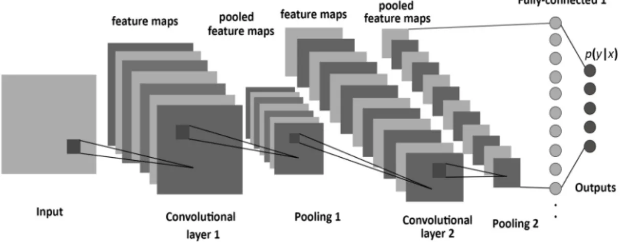
CNN [54] is a subclass of neural networks that takes advantage of the spatial structure of the inputs. CNN models have a standard structure consisting of alternating convolutional layers and pooling layers (often each pooling layer is placed after a convolutional layer). The last layers are a small number of fully-connected layers, and the final layer is a softmax classifier as shown in Figure1. CNNs are usually trained by backpropagation via Stochastic Gradient Decent (SGD) to find weights and biases that minimize certain loss function in order to map the arbitrary inputs to the targeted outputs as closely as possible.
The convolutional layer is comprised of a set of learnable kernels or filters which aim to extract local features from the input. Each kernel is used to calculate a feature map. The units of the feature maps can only connect to a small region of the input, called the receptive field. A new feature map is typically generated by sliding a filter over the input and computing the dot product (which is similar to the convolution operation), followed by a non-linear activation function to introduce non-linearity into the model. All units share the same weights (filters) among each feature map. The advantage of sharing weights is the reduced number of parameters and the ability to detect the same feature, regardless of its location in the inputs [55].
Several nonlinear activation functions are available, such as sigmoid, tanh, and ReLU. However, ReLU [f(x) = max (0, x)] is preferable because it makes training faster relative to the others [3,56]. The size of the output feature map is based on the filter size and stride, so when we convolve the input image with a size of (H×H) over a filter with a size of (F×F) and a stride of (S), then the output size of (W×W) is given by: W= H−F S +1 (1)
EntropyEntropy 2017,2017, 19, 242 19, 242 5 of 205 of 20
Figure 1. The structure of a CNN, consisting of convolutional, pooling, and fully-connected layers.
The pooling, or down-sampling layer, reduces the resolution of the previous feature maps. Pooling produces invariance to a small transformation and/or distortion. Pooling splits the inputs into disjoint regions with a size of (R × R) to produce one output from each region [57]. Pooling can be max or average based [58]. If a given input with a size of (W × W) is fed to the pooling layer, then the output size will be obtained by:
= W (2)
The top layers of CNNs are one or more fully-connected layers similar to a feed-forward neural network, which aims to extract the global features of the inputs. Units of these layers are connected to all hidden units in the preceding layer. The very last layer is a softmax classifier, which estimates the posterior probability of each class label over K classes as shown in Equation (3) [27]:
=∑exp(− )
exp( ) (3)
3.2. CNN Architecture Design
In this framework, our learning algorithm for the CNN (Λ) is specified by a structural hyperparameter λ which encapsulates the design of the CNN architecture as follows:
= ( , , , , )
,, ( )
, (4)where λ∈ Ψ defines the domain for each hyperparameter, ( ) is the number of convolutional layers, and ( ) is the number of fully-connected layers (i.e., the depth = + ). Constructing any convolutional layer requires four hyperparameters that must be identified. For example, for convolutional layer i: is the number of filters, is the filter size (receptive field size), and defines the pooling locations and sizes. If is equal to one, this means there is no pooling layer placed after convolutional layer i; otherwise, there is a pooling layer after convolutional layer i and the value defines the pooling region size. is stride step. is the number of units in fully-connected layer j. We also use ℓ(Λ, , ) to refer to the validation loss (e.g., classification error) obtained when we train model Λwith the training set ( ) and evaluate it on the validation set ( ). The purpose of our framework is to optimize the combination of structural hyperparameters λ* that designs the architecture for a given dataset automatically, resulting in a minimization of the classification error as follows:
∗=
ℓ(Λ,
,
)
(5) Figure 1.The structure of a CNN, consisting of convolutional, pooling, and fully-connected layers.
The pooling, or down-sampling layer, reduces the resolution of the previous feature maps. Pooling produces invariance to a small transformation and/or distortion. Pooling splits the inputs into disjoint regions with a size of (R×R) to produce one output from each region [57]. Pooling can be max or average based [58]. If a given input with a size of (W×W) is fed to the pooling layer, then the output size will be obtained by:
P= W R (2) The top layers of CNNs are one or more fully-connected layers similar to a feed-forward neural network, which aims to extract the global features of the inputs. Units of these layers are connected to all hidden units in the preceding layer. The very last layer is a softmax classifier, which estimates the posterior probability of each class label overKclasses as shown in Equation (3) [27]:
yi= exp(−zi)
∑K
j=iexp zj
(3)
3.2. CNN Architecture Design
In this framework, our learning algorithm for the CNN (Λ) is specified by a structural hyperparameterλwhich encapsulates the design of the CNN architecture as follows:
λ= (λi1,λi2,λi3, ,λ4i)i=1,Mc, (λ1j)j=1,N f (4) whereλ∈Ψdefines the domain for each hyperparameter,(MC)is the number of convolutional layers, and
(NF)is the number of fully-connected layers (i.e., the depth =MC+Nf). Constructing any convolutional layer requires four hyperparameters that must be identified. For example, for convolutional layeri:λi1is the number of filters,λi2is the filter size (receptive field size), andλi3defines the pooling locations and sizes. Ifλi3is equal to one, this means there is no pooling layer placed after convolutional layeri; otherwise, there is a pooling layer after convolutional layeriand the valueλi3defines the pooling region size.λi4is stride step.λ5j is the number of units in fully-connected layerj. We also use`(Λ,TTR,TV)to refer to the validation loss (e.g., classification error) obtained when we train modelΛwith the training set (TTR) and evaluate it on the validation set (TV). The purpose of our framework is to optimize the combination of structural hyperparametersλ* that designs the architecture for a given dataset automatically, resulting in a minimization of the classification error as follows:
Entropy2017,19, 242 6 of 20
4. Framework Model
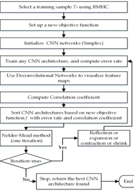
In this section, we present details of the framework model consisting of deconvolutional networks, correlation coefficient, objective function, NMM, and web services for obtaining a high-performing CNN architecture for a given dataset. For large datasets, we use instance selection and statistics to determine the optimal, reduced training dataset as a preprocessing step. A general framework flowchart and components are shown in Figure2.
Entropy 2017, 19, 242 6 of 20
4. Framework Model
In this section, we present details of the framework model consisting of deconvolutional networks, correlation coefficient, objective function, NMM, and web services for obtaining a high-performing CNN architecture for a given dataset. For large datasets, we use instance selection and statistics to determine the optimal, reduced training dataset as a preprocessing step. A general framework flowchart and components are shown in Figure 2.
Figure 2. General components and a flowchart of our framework for discovering a high-performing CNN architecture.
4.1. Reducing the Training Set
Training deep CNN architectures with a large training set involves a high computational time. The large dataset may contain redundant or useless images. In machine learning, a common approach of dealing with a large dataset is instance selection, which aims to choose a subset or sample ( ) of the training set ( ) to achieve acceptable accuracy as if the whole training set was being used. Many instance selection algorithms have been proposed and reviewed in [59]. Albelwi and Mahmood [60] evaluated and analyzed the performance of different instance selection algorithms on CNNs. In this framework, for very large datasets, we employ instance selection based on Random Mutual Hill Climbing (RMHC) [61] as a preprocessing step to select the training sample ( ) which will be used during the exploration phase to find a high-performing architecture. The reason for selecting RMHC is that the user can predefine the size of the training sample, which is not possible with other algorithms. We employ statistics to determine the most representative sample size, which is critical to obtaining accurate results.
In statistics, calculating the optimal size of a sample depends on two main factors: the margin of error and confidence level. The margin of error defines the maximum range of error between the results of the whole population (training set) and the result of a sample (training sample). The confidence level measures the reliability of the results of the training sample, which reflects the training set. Typical confidence level values are 90%, 95%, or 99%. We use a 95% confidence interval in determining the optimal size of a training sample (based on RHMC) to represent the whole training set.
Figure 2.General components and a flowchart of ourframework for discovering a high-performing CNN architecture.
4.1. Reducing the Training Set
Training deep CNN architectures with a large training set involves a high computational time. The large dataset may contain redundant or useless images. In machine learning, a common approach of dealing with a large dataset is instance selection, which aims to choose a subset or sample(TS)of the training set(TTR)to achieve acceptable accuracy as if the whole training set was being used. Many instance selection algorithms have been proposed and reviewed in [59]. Albelwi and Mahmood [60] evaluated and analyzed the performance of different instance selection algorithms on CNNs. In this framework, for very large datasets, we employ instance selection based on Random Mutual Hill Climbing (RMHC) [61] as a preprocessing step to select the training sample (TS) which will be used during the exploration phase to find a high-performing architecture. The reason for selecting RMHC is that the user can predefine the size of the training sample, which is not possible with other algorithms. We employ statistics to determine the most representative sample size, which is critical to obtaining accurate results.
In statistics, calculating the optimal size of a sample depends on two main factors: the margin of error and confidence level. The margin of error defines the maximum range of error between the results of the whole population (training set) and the result of a sample (training sample). The confidence level measures the reliability of the results of the training sample, which reflects the training set. Typical confidence level values are 90%, 95%, or 99%. We use a 95% confidence interval in determining the optimal size of a training sample (based on RHMC) to represent the whole training set.
Entropy2017,19, 242 7 of 20
4.2. CNN Feature Visualization Methods
Recently, there has been a dramatic interest in the use of visualization methods to explore the inner operations of a CNN, which enables us to understand what the neurons have learned. There are several visualization approaches. A simple technique called layer activation shows the activations of the feature maps [62] as a bitmap. However, to trace what has been detected in a CNN is very difficult. Another technique is activation maximization [63], which retrieves the images that maximally activate the neuron. The limitation of this method is that the ReLU activation function does not always have a semantic meaning by itself. Another technique is deconvolutional network [14], which shows the parts of the input image that are learned by a given feature map. The deconvolutional approach is selected in our work because it results in a more meaningful visualization and also allows us to diagnose potential problems with the architecture design.
Deconvolutional Networks
Deconvolutional networks (deconvnet) [14] are designed to map the activities of a given feature in higher layers to go back into the input space of a trained CNN. The output of deconvnet is a reconstructed image that displays the activated parts of the input image learned by a given feature map. Visualization is useful for evaluating the behavior of a trained architecture because a good visualization indicates that a CNN is learning properly, whereas a poor visualization shows ineffective learning. Thus, it can help tune the CNN architecture design accordingly in order to enhance its performance. We attach a deconvnet layer with each convolutional layer similar to [14], as illustrated at the top of Figure3. Deconvnet applies the same operations of a CNN but in reverse, including unpooling, a non-linear activation function (in our framework, ReLU), and filtering.
Entropy 2017, 19, 242 7 of 20
4.2. CNN Feature Visualization Methods
Recently, there has been a dramatic interest in the use of visualization methods to explore the inner operations of a CNN, which enables us to understand what the neurons have learned. There are several visualization approaches. A simple technique called layer activation shows the activations of the feature maps [62] as a bitmap. However, to trace what has been detected in a CNN is very difficult. Another technique is activation maximization [63], which retrieves the images that maximally activate the neuron. The limitation of this method is that the ReLU activation function does not always have a semantic meaning by itself. Another technique is deconvolutional network [14], which shows the parts of the input image that are learned by a given feature map. The deconvolutional approach is selected in our work because it results in a more meaningful visualization and also allows us to diagnose potential problems with the architecture design.
Deconvolutional Networks
Deconvolutional networks (deconvnet) [14] are designed to map the activities of a given feature in higher layers to go back into the input space of a trained CNN. The output of deconvnet is a reconstructed image that displays the activated parts of the input image learned by a given feature map. Visualization is useful for evaluating the behavior of a trained architecture because a good visualization indicates that a CNN is learning properly, whereas a poor visualization shows ineffective learning. Thus, it can help tune the CNN architecture design accordingly in order to enhance its performance. We attach a deconvnet layer with each convolutional layer similar to [14], as illustrated at the top of Figure 3. Deconvnet applies the same operations of a CNN but in reverse, including unpooling, a non-linear activation function (in our framework, ReLU), and filtering.
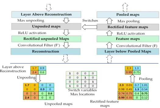
Figure 3. The top part illustrates the deconvnet layer on the left, attached to the convolutional layer on the right. The bottom part illustrates the pooling and unpooling operations [14].
The deconvnet process involves a standard forward pass through the CNN layers until it reaches the desired layer that contains the selected feature map to be visualized. In a max pooling operation, it is important to record the locations of the maxima of each pooling region in switch variables because max pooling is non-invertible. All feature maps in a desired layer will be set to zero except the one that is to be visualized. Now we can use deconvnet operations to go back to the input space for performing reconstruction. Unpooling aims to reconstruct the original size of the activations by using switch variables to return the activation from the layer above to its original position in the
Figure 3.The top part illustrates the deconvnet layer on the left, attached to the convolutional layer on the right. The bottom part illustrates the pooling and unpooling operations [14].
The deconvnet process involves a standard forward pass through the CNN layers until it reaches the desired layer that contains the selected feature map to be visualized. In a max pooling operation, it is important to record the locations of the maxima of each pooling region in switch variables because max pooling is non-invertible. All feature maps in a desired layer will be set to zero except the one that is to be visualized. Now we can use deconvnet operations to go back to the input space for performing reconstruction. Unpooling aims to reconstruct the original size of the activations by using switch
Entropy2017,19, 242 8 of 20
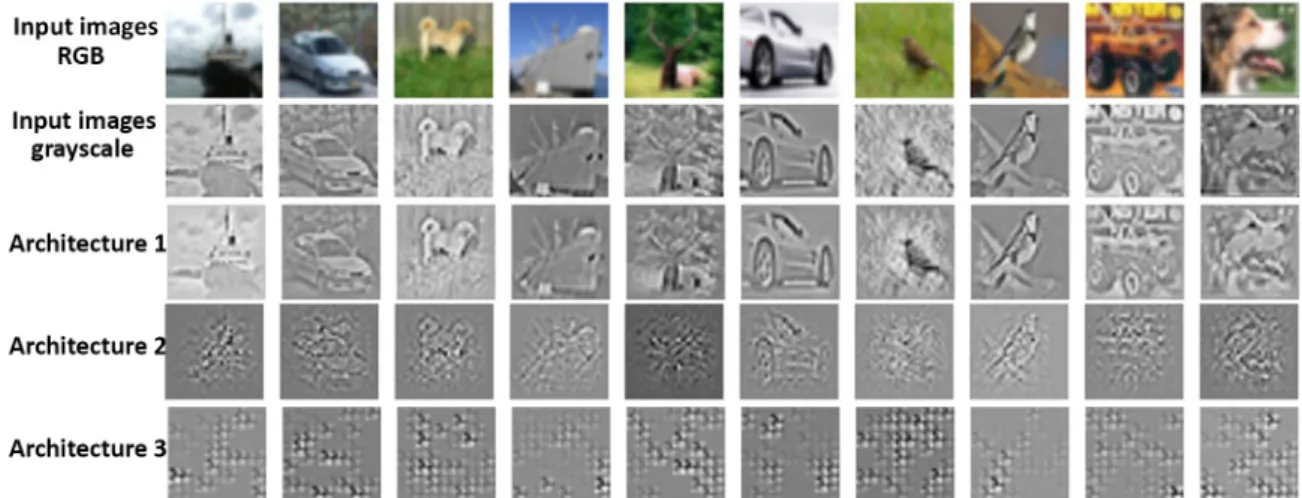
variables to return the activation from the layer above to its original position in the pooling layer, as shown at the bottom of Figure3, thereby preserving the structure of the stimulus. Then, the output of the unpooling passes through the ReLU function. Finally, deconvnet applies a convolution operation on the rectified, unpooled maps with transposed filters in the corresponding convolutional layer. Consequently, the result of deconvnet is a reconstructed image that contains the activated pieces of the input that were learnt. Figure4displays the visualization of different CNN architectures. As shown, the quality of the visualization varies from one architecture to another compared to the original images in grayscale. For example, CNN architecture 1 shows very good visualization; this gives a positive indication about the architecture design. On the other hand, CNN architecture 3 shows poor visualization, indicating this architecture has potential problems and did not learn properly.
The visualization of feature maps is thus useful in diagnosing potential problems in CNN architectures. This helps in modifying an architecture to enhance its performance, and also evaluating different architectures with criteria besides the classification error on the validation set. Once the reconstructed image is obtained, we use the correlation coefficient to measure the similarity between the input image and its reconstructed image in order to evaluate the reconstruction’s representation quality.
Entropy 2017, 19, 242 8 of 20
pooling layer, as shown at the bottom of Figure 3, thereby preserving the structure of the stimulus. Then, the output of the unpooling passes through the ReLU function. Finally, deconvnet applies a convolution operation on the rectified, unpooled maps with transposed filters in the corresponding convolutional layer. Consequently, the result of deconvnet is a reconstructed image that contains the activated pieces of the input that were learnt. Figure 4 displays the visualization of different CNN architectures. As shown, the quality of the visualization varies from one architecture to another compared to the original images in grayscale. For example, CNN architecture 1 shows very good visualization; this gives a positive indication about the architecture design. On the other hand, CNN architecture 3 shows poor visualization, indicating this architecture has potential problems and did not learn properly.
The visualization of feature maps is thus useful in diagnosing potential problems in CNN architectures. This helps in modifying an architecture to enhance its performance, and also evaluating different architectures with criteria besides the classification error on the validation set. Once the reconstructed image is obtained, we use the correlation coefficient to measure the similarity between the input image and its reconstructed image in order to evaluate the reconstruction’s representation quality.
Figure 4. Visualization from the last convolutional layer for three different CNN architectures. Grayscale input images are visualized after preprocessing.
4.3. Correlation Coefficient
The correlation coefficient (Corr) [64] measures the level of similarity between two images or independent variables. The correlation coefficient is maximal when two images are highly similar. The correlation coefficient between two images A and B is given by:
( , ) =1 ( − ) ( − ) (6)
where and are the averages of A and B respectively, denotes the standard deviation of A, and denotes the standard deviation of B. Fast Fourier Transform (FFT) provides an alternative approach to calculate the correlation coefficient with a high computational speed as compared to Equation (6) [65,66]. The correlation coefficient between A and B is computed by locating the maximum value of the following equation:
( , ) = ℱ [ℱ( ) ∘ ℱ∗( )] (7) where ℱ is an FFT for a two-dimensional image, ℱ indicates inverse FFT, * is the complex conjugate, and ∘ implies element by element multiplication. This approach reduces the time complexity of the computing correlation from ( ) to ( log ). Once the training of the CNN
Figure 4. Visualization from the last convolutional layer for three different CNN architectures. Grayscale input images are visualized after preprocessing.
4.3. Correlation Coefficient
The correlation coefficient (Corr) [64] measures the level of similarity between two images or independent variables. The correlation coefficient is maximal when two images are highly similar. The correlation coefficient between two imagesAandBis given by:
Corr(A,B) = 1 n n
∑
i=1 (ai−b σa ) (ai−b σb ) (6)where aand bare the averages of A andB respectively, σa denotes the standard deviation of A, andσb denotes the standard deviation ofB. Fast Fourier Transform (FFT) provides an alternative approach to calculate the correlation coefficient with a high computational speed as compared to Equation (6) [65,66]. The correlation coefficient between A and B is computed by locating the maximum value of the following equation:
Corr(A,B) =F−1[F(A)◦ F∗(B)] (7) whereF is an FFT for a two-dimensional image,F−1indicates inverse FFT, * is the complex conjugate,
Entropy2017,19, 242 9 of 20
computing correlation fromO N2
toO(N log N). Once the training of the CNN is complete, we compute the error rate (Err) on the validation set, and chooseNfm feature maps at random from the last layer to visualize their learned parts using deconvnet. The motivation behind selecting the last convolutional layer is that it should show the highest level of visualization as compared to preceding layers. We chooseNimgimages from the training sample at random to test the deconvnet. The correlation coefficient is used to calculate the similarity between the input imagesNimgand their reconstructions. Since each image ofNimghas a correlation coefficient (Corr) value, the results of all Corrvalues are accumulated in a scalar value called (CorrRes). Algorithm 1 summarizes the processing procedure for training a CNN architecture:
Algorithm 1.Processing Steps for Training a Single CNN Architecture.
1: Input: training sampleTS, validation setTV,Nfmfeature maps, andNimgimages
2: Output:ErrandCorrRes
3: Train CNN architecture design using SGD 4: Compute error rate (Err) on validation setTV
5: CorrRes=0
6: Fori= 1 toNfm
7: Pick a feature mapfmat random from the last convolutional layer 8: Forj= 1 toNimg
9: Use deconvnet to visualize a selected feature mapfmon imageNimg[j]
10: CorrRes=CorrRes+ correlation coefficient (Nimg[j], reconstructed image)
11: ReturnErrandCorrRes 4.4. Objective Function
Existing works on hyperparameter optimization for deep CNNs generally use the error rate on the validation set to decide whether one architecture design is better than another during the exploration phase. Since there is a variation in performance on the same architecture from one validation set to another, the model design cannot always be generalized. Therefore, we present a new objective function that exploits information from the error rate (Err) on the validation set as well as the correlation results(CorrRes)obtained from deconvnet. The new objective function can be written as:
f(λ) =η(1−CorrRes) + (1−η)Err (8) whereηis a correlation coefficient parameter measuring the importance ofErrandCorrRes. The key reason to subtractCorrResfrom one is to minimize both terms of the objective function. We can set up the objective function in Equation (8) as an optimization problem that needs to be minimized. Therefore, the objective function aims to find a CNN architecture that minimizes the classification error and provides a high level of visualization. We use the NMM to guide our search into a promising direction for discovering iteratively better-performing CNN architecture designs by minimizing the proposed objective function.
4.5. Nelder Mead Method
The Nelder-Mead algorithm (NMM), or simplex method [67], is a direct search technique widely used for solving optimization problems based on the values of the objective function when the derivative information is unknown. NMM uses a concept called a simplex, which is a geometric shape consisting ofn+ 1 vertices for optimizingnhyperparameters. First, NMM creates an initial simplex that is generated randomly. In this framework, let [Z1,Z2, . . . ,Zn+1] refer to simplex vertices, where
each vertex presents a CNN architecture. The vertices are sorted in ascending order based on the value of objective functionsf(Z1)≤f(Z2)≤. . . ≤f(Zn+1) so that Z1is the best vertex, which provides the
Entropy2017,19, 242 10 of 20
best CNN architecture, andZn+1is the worst vertex. NMM seeks to find the best hyperparametersλ*
that designs a CNN architecture that minimizes the objective function in Equation 8 as follows: λ∗ =arg min
λ∈Ψ
f(λ) (9)
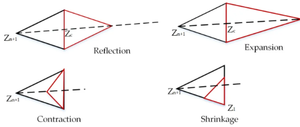
The search is performed based on four basic operations: reflection, expansion, contraction, and shrinkage, as shown in Figure5. Each is associated with a scalar coefficient ofα(reflection),β (expansion),γ(contraction), andδ(shrinkage). In each iteration, NMM tries to update a current simplex to generate a new simplex which decreases the value of the objective function. NMM replaces the worst vertex with the best that has been found from reflected, expanded or contracted vertices. Otherwise, all vertices of the simplex, except the best, will shrink around the best vertex. These processes are repeated until the stop criterion is accomplished. The vertex producing the lowest objective function value is the best solution that is returned. The main challenge in finding a high-performing CNN architecture is the execution time and, correspondingly, the number of computing resources required. We can apply our optimization objective function with any derivative-free algorithm such as genetic algorithms, particle swarm optimization, Bayesian optimization, and the Nelder-Mead method, etc. The reason for selecting NMM is that it is faster than other derivative-free optimization algorithms, because in each iteration, only a few vertices are evaluated. Further, NMM is easy to parallelize with a small number of workers to accelerate the execution time.
During the calculation of any vertex of NMM, we added some constraints to make the output values positive integers. The value ofCorrResis normalized between the minimum and maximum value of the error rate in each iteration of NMM. This is critical because it affects the value ofηin Equation (8).
Entropy 2017, 19, 242 10 of 20
best CNN architecture, and Zn+1 is the worst vertex. NMM seeks to find the best hyperparameters λ* that designs a CNN architecture that minimizes the objective function in Equation 8 as follows:
∗
= arg min
∈
( )
(9)The search is performed based on four basic operations: reflection, expansion, contraction, and shrinkage, as shown in Figure 5. Each is associated with a scalar coefficient of α (reflection), β
(expansion), γ (contraction), and δ (shrinkage). In each iteration, NMM tries to update a current simplex to generate a new simplex which decreases the value of the objective function. NMM replaces the worst vertex with the best that has been found from reflected, expanded or contracted vertices. Otherwise, all vertices of the simplex, except the best, will shrink around the best vertex. These processes are repeated until the stop criterion is accomplished. The vertex producing the lowest objective function value is the best solution that is returned. The main challenge in finding a high-performing CNN architecture is the execution time and, correspondingly, the number of computing resources required. We can apply our optimization objective function with any derivative-free algorithm such as genetic algorithms, particle swarm optimization, Bayesian optimization, and the Nelder-Mead method, etc. The reason for selecting NMM is that it is faster than other derivative-free optimization algorithms, because in each iteration, only a few vertices are evaluated. Further, NMM is easy to parallelize with a small number of workers to accelerate the execution time.
During the calculation of any vertex of NMM, we added some constraints to make the output values positive integers. The value of is normalized between the minimum and maximum value of the error rate in each iteration of NMM. This is critical because it affects the value of in Equation (8).
Figure 5. Nelder Mead method operations: reflection, expansion, contraction, and shrinkage. 4.6. AcceleratingProcesssing Time with Parallelism
Since serial NMM executes the vertices sequentially one vertex at a time, the optimization processing time is very expensive for deep CNN models. For this reason, it is necessary to utilize parallel computing to reduce the execution time; NMM provides a high degree of parallelism since there are no dependences between the vertices. In most iterations of NMM, the worst vertex is replaced with either the reflected, expanded, or contracted vertex. Therefore, these vertices can be evaluated simultaneously on distributed workers. We implement a synchronous master-slave NMM model, which distributes the running of several vertices on workers while the master machine controls the whole optimization procedure. The master cannot move to the next step until all of the workers finish their tasks. A synchronous NMM has the same properties as a serial NMM, but it works faster.
Recently, web services [68] provide a powerful technology for interacting between distributed applications written in different programming languages and running on heterogeneous platforms, such as operating systems and hardware over the internet [69,70]. There are two popular methods for building a web service application to interact between distributed computers: Simple Object Access Protocol (SOAP) and Representational State Transfer (RESTful). We use RESTful [71] to create
Figure 5.Nelder Mead method operations: reflection, expansion, contraction, and shrinkage. 4.6. AcceleratingProcesssing Time with Parallelism
Since serial NMM executes the vertices sequentially one vertex at a time, the optimization processing time is very expensive for deep CNN models. For this reason, it is necessary to utilize parallel computing to reduce the execution time; NMM provides a high degree of parallelism since there are no dependences between the vertices. In most iterations of NMM, the worst vertex is replaced with either the reflected, expanded, or contracted vertex. Therefore, these vertices can be evaluated simultaneously on distributed workers. We implement a synchronous master-slave NMM model, which distributes the running of several vertices on workers while the master machine controls the whole optimization procedure. The master cannot move to the next step until all of the workers finish their tasks. A synchronous NMM has the same properties as a serial NMM, but it works faster.
Recently, web services [68] provide a powerful technology for interacting between distributed applications written in different programming languages and running on heterogeneous platforms, such as operating systems and hardware over the internet [69,70]. There are two popular methods
Entropy2017,19, 242 11 of 20
for building a web service application to interact between distributed computers: Simple Object Access Protocol (SOAP) and Representational State Transfer (RESTful). We use RESTful [71] to create web services because it is simple to implement as well as lightweight, fast, and readable by humans; unlike RESTful, SOAP is difficult to develop, requires tools and is heavyweight. A RESTful service submits CNN hyperparameters into worker machines. Each worker builds and trains the architecture, computes the error rate and the correlation coefficient results, and returns both results to the master computer. Moreover, when shrinkage is selected, we run three vertices at the same time. This has a significant impact in reducing the computation time. Our framework is described in Algorithm 2, which details and integrates the techniques for finding the best CNN architecture.
Algorithm 2. The Proposed Framework Pseudocode.
1: Input:n: Number of hyperparameters
2: Output:best vertex (Z[1]) found that minimizes the objective function in equation 8
3: Determine training sampleTSusing RMHC
4: Initialize the Simplex vertices (Z1:n+1) randomly from Table1 5: L=d(n+1)/3e# 3 is the number of workers
6: Forj= 1 toL
7: Train each 3 vertices ofZ1,n+1in parallel according to Algorithm 1 8: Forl= 1 to Max_ _iterations:
9: Normalize values ofCorrResbetween themaxandminofErrof vertices of (Z) 10: Computef(Zi)based on Equation (8). for all verticesi = 1:n+1
11: Z= order the vertices so thatf(Z1)≤f(Z2), . . . ,<f(Zn+1). 12: SetB=Z1,A=Zn,W=Zn+1
13: Compute the centroidCof vertices without considering the worst vertex:C= 14: 1n∑n
i=1Zi
15: Compute reflected vertex:R=C+α(C−W)
16: Compute Expanded vertexE=R+γ(R−C)
17: Compute Contracted vertexCon=ρR+ (1−ρ)C
18: TrainR,E, andConsimultaneously on workers 1,2, and 3 according to Algorithm 1 19: NormalizeCorrResofR, E, andConbetween themaxandminofErrof vertices of (Z) 20: Computef(R), f(E), andf(con)based on Equation (8)
21: Iff(B) >R<W 22: Zn+1= W 23: Else Iff(R)≤f(B) 24: Iff(E) <f(R) 25: Zn+1= E 26: Else 27: Zn+1=R 28: Else 29: d= true 30: Iff(R)≤f(A) 31: Iff(Con)≤f(R) 32: Zn+1=Con 33: d= false 34: Ifd= true
35: shrink toward the best vertex direction 36: L =dn/3e
37: Fork= 2 ton+1: # do not include the best vertex 38: Zk=B+σ(Zk−B)
39: Forj= 1 to L:
40: Train each 3 vertices of(Z2:n+1) in parallel on workers 1, 2, and 3 according 41: to Algorithm 1
Entropy2017,19, 242 12 of 20
5. Results and Discussion 5.1. Datasets
The evaluation of our framework is done on the CIFAR-10, CIFAR-100, and MNIST datasets. The CIFAR-10 dataset [72] has 10 classes of 32×32 color images. There are 50K images for training, and 10K images for testing. CIFAR-100 [72] is the same size as CIFAR-10, except the number of classes is 100. Each class of CIFAR-100 contains 500 images for training and 100 for testing, which makes it more challenging. We apply the same preprocessing on both the CIFAR-10 and CIFAR-100 datasets, i.e., we normalize the pixels in each image by subtracting the mean pixel value and dividing it by the standard deviation. Then we apply ZCA whitening with an epsilon value of 0.01 for both datasets. Another dataset used is MNIST [54], which consists of the handwritten digits 0–9. Each digit image is 28×28 in size, and there are 10 classes. MNIST contains 60K images for training and 10K for testing. The normalization is done similarly to CIFAR-10 and CIFAR-100, without the ZCA whitening. 5.2. Experimental Setup
Our framework is implemented in Python using the Theano library [73] to train the CNN models. Theano provides automatic differentiation capabilities to compute gradients and allows the use of GPU to accelerate the computation. During the exploration phase via NMM, we select a training sampleTS using an RMHC algorithm with a sample size based on a margin error of 1 and confidence level of 95%. Then, we select 8000 images randomly from (TTR–TS) for validation setTV.
Training Settings: We use SGD to train CNN architectures. The final learning rate is set to 0.08 for 25 epochs and 0.008 for the last epochs; these values are selected after doing a small grid search among different values on the validation set. We set the batch size to 32 images and the weight decay to 0.0005. The weights of all layers are initialized according to the Xavier initialization technique [42], and biases are set to zero. The advantage of Xavier initialization is that it makes the network converge much faster than other approaches. The weight sets it produces are also more consistent than those produced by other techniques. We apply ReLU with all layers and employ early stopping to prevent overfitting in the performance of the validation set. Once the error rate increases or saturates for a number of iterations, the model stops the training procedure. Since the training time of a CNN is expensive and some designs perform poorly, early stopping saves time by terminating poor architecture designs early. Dropout [11] is implemented with fully-connected layers with a rate of 0.5. It has proven to be an effective method in combating overfitting in CNNs, and a rate of 0.5 is a common practice. During the exploration phase of NMM, each of the experiments are run with 35 epochs. Once the best CNN architecture is obtained, we train it with the training setTTRand evaluate it on a testing set with
200 epochs.
Nelder Mead Settings:The total number of hyperparametersnis required to construct the initial simplex withn+ 1 vertices. However, this number is different for each dataset. In order to define nfor a given dataset, we initialize 80 random CNN architectures as an additional step to return the maximum number of convolutional layers (Cmax) in all architectures. Then, according to Equation (4), the number of hyperparametersnis given by:
n=Cmax×4 + the max number of fully-connected layers. (10) NMM will then initialize a new initial simplex (Z0) withn+ 1 vertices. For all datasets, we set the
value of the correlation coefficient parameter toη= 0.20. We select at randomNfm= 10 feature maps from the last convolutional layer to visualize their learned features andNimg= 100 images from the training sample to assess the visualization. The number of iterations for NMM is 25.
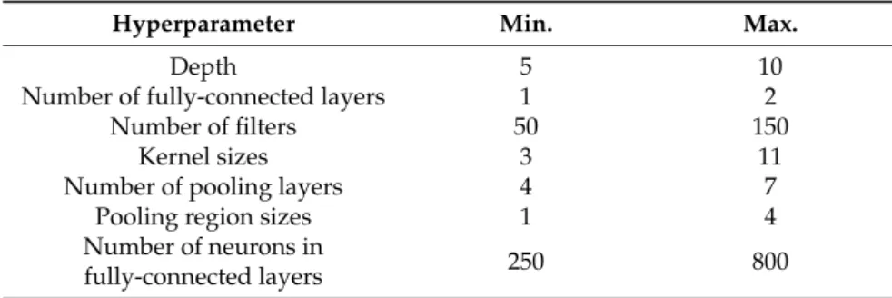
Table1summarizes the hyperparameter initialization ranges for the initial simplex vertices (CNN architectures) of NMM. The number of convolutional layers is calculated automatically by subtracting the depth from the number of fully-connected layers. However, the actual number of
Entropy2017,19, 242 13 of 20
convolutional layers is controlled by the size of the input image, filter sizes, strides and pooling region sizes according to Equations (1) and (2). Some CNN architectures may not result in feasible configurations based on initial hyperparameter selections, because after a set of convolutional layers, the size of feature maps (W) or pooling (P) may become <1, so the higher convolutional layers will be automatically eliminated. Therefore, the depth varies through CNN architectures; this will be helpful to optimize the depth. There is no restriction on fully-connected layers. For example, the hyperparameters of the following CNN architecture are initialized randomly from Table1, which consists of six convolutional layers and two fully-connected layers as follows:
[[85, 3, 2, 1], [93, 5, 1, 1], [72, 3, 2, 2], [61, 7, 2, 1], [83, 7, 2, 3], [69, 3, 2, 3], [715, 554]]
For an input image of size 32×32, the framework designs a CNN architecture with only three convolutional layers because the output size of a fourth layer would be negative. Thus, the remaining convolutional layers from the fourth layer will be deleted automatically by setting them to zeros as shown below:
[[85, 3, 2, 1], [93, 5, 1, 1], [72, 3, 2, 2], [0, 0, 0, 0], [0, 0, 0, 0], [0, 0, 0, 0], [715, 554]] Table 1.Hyperparameter initialization ranges.
Hyperparameter Min. Max.
Depth 5 10
Number of fully-connected layers 1 2
Number of filters 50 150
Kernel sizes 3 11
Number of pooling layers 4 7
Pooling region sizes 1 4
Number of neurons in
fully-connected layers 250 800
5.3. Results and Discussion
First, we validate the effectiveness of the proposed objective function compared to the error rate objective function. After initializing a simplex (Z0) of NMM, we optimize the architecture using
NMM based on the proposed objective function (error rate as well as visualization). Then, from the same initialization (Z0), we execute the NMM based on the error rate objective function alone
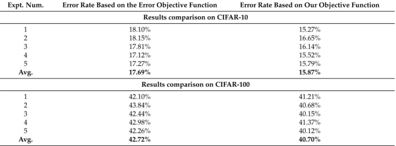
by settingη to zero. Table 2 compares the error rate of five experiment runs obtained from the best CNN architectures found using the objective functions presented above on the CIFAR-10 and CIFAR-100 datasets respectively. The results illustrate that our new objective function outperforms the optimization obtained from the error rate objective function alone. The error rate averages of 15.87% and 40.70% are obtained with our objective function, as compared to 17.69% and 42.72% when using the error rate objection function alone, on CIFAR-10 and CIAFAR-100 respectively. Our objective function searches the architecture that minimizes the error and improves the visualization of learned features, which impacts the search space direction, and thus produces a better CNN architecture.
Entropy2017,19, 242 14 of 20
Table 2.Error rate comparisons between the top CNN architectures obtained by our objective function and the error rate objective function via NMM.
Expt. Num. Error Rate Based on the Error Objective Function Error Rate Based on Our Objective Function Results comparison on CIFAR-10
1 18.10% 15.27% 2 18.15% 16.65% 3 17.81% 16.14% 4 17.12% 15.52% 5 17.27% 15.79% Avg. 17.69% 15.87%
Results comparison on CIFAR-100
1 42.10% 41.21% 2 43.84% 40.68% 3 42.44% 40.15% 4 42.98% 41.37% 5 42.26% 40.12% Avg. 42.72% 40.70%
We also compare the performance of our approach with existing methods that did not apply data augmentation, namely hand-designed architectures by experts, random search, genetic algorithms, and Bayesian optimization. For CIFAR-10, [72] reported that the best hand-crafted CNN architecture design tuned by human experts obtained an 18% error rate. In [22], genetic algorithms are used to optimize filter sizes and the number of filters for convolutional layers; it achieved a 25% error rate. In [74], SMAC is implemented to optimize the number of filters, filter sizes, pooling region sizes, and fully-connected layers with a fixed depth. They achieved an error rate of 17.47%. As shown in Table3, our method outperforms others with an error rate of 15.27%. For CIFAR-100, we implement random search by picking CNN architectures from Table1, and the lowest error rate that we obtained is 44.97%. In [74], which implemented SMAC, an error rate of 42.21% is reported. Our approach outperforms these methods with an error rate of 40.12%, as shown in Table3.
Table 3.Error rate comparison for different methods of designing CNN architectures on CIFAR-10 and CIFAR-100. These results are achieved without data augmentation.
Method CIFAR-10 CIFAR-100
Human experts design [72] 18%
-Random search (our implementation) 21.74% 44.97%
Genetic algorithms [22] 25%
-SMAC [74] 17.47% 42.21%
Our approach 15.27% 40.12%
In each iteration of NMM, a better-performing CNN architecture is potentially discovered that minimizes the value of the objective function; however, it can get stuck in a local minimum. Figure6
shows the value of the best CNN architecture versus the iteration using both objective functions, i.e., the objective function based on error rate alone and our new, combined objective function. In many iterations, NMM paired with the error rate objective function is unable to pick a new, better-performing CNN architecture and gets stuck in local minima early. The number of architectures that yield a higher performance during the optimization process is only 12 and 10 out of 25, on CIFAR-10 and CIFAR-100 respectively. In contrast, NMM with our new objective function is able to explore better-performing CNN architectures with a total number of 19 and 17 architectures on CIFAR-10 and CIFAR-100 respectively, and it does not get stuck early in a local minimum, as shown in Figure6b. The main hallmark of our new objective function is that it is based on both the error rate and the correlation coefficient (obtained from the visualization of the CNN via deconvnet), which gives us flexibility to sample a new architecture, thereby improving the performance.
Entropy2017,19, 242 15 of 20
Entropy 2017, 19, 242 15 of 20
correlation coefficient (obtained from the visualization of the CNN via deconvnet), which gives us flexibility to sample a new architecture, thereby improving the performance.
(a) (b)
Figure 6. Objective functions progress during the iterations of NMM. (a) CIFAR-10; (b) CIFAR-100.
We further investigated the characteristics of the best CNN architectures obtained by both objective functions using NMM on CIFAR-10 and CIFAR-100. We took the average of the hyperparameters of the best CNN architectures. As shown in Figure 7a, CNN architectures based on the proposed framework tend to be deeper compared to architectures obtained by the error rate objective function alone. Moreover, some convolutional layers are not followed by pooling layers. As a result, we found that reducing the number of pooling layers shows a better visualization, and results in adding more layers. On the other hand, the architectures obtained by the error objective function alone result in every convolutional layer being followed by a pooling layer.
Figure 7. The average of the best CNN architectures obtained by both objective functions. (a) The architecture averages for our framework; (b) The architecture averages for the error rate objective function.
We compare the run-time of NMM on a single computer with a parallel NMM algorithm on three distributed computers. The running time decreases almost linearly (3×) as the number of workers increases, as shown in Table 4. In a synchronous master-slave NMM model, the master cannot move to the next step until all of the workers finish their jobs, so other workers wait until the biggest CNN architecture training is done. This creates a minor delay. In addition, the run-time of
Corr based on Equation (6) is 0.05 s; when based on FFT in Equation (7), it is 0.01 s.
Figure 6.Objective functions progress during the iterations of NMM. (a) CIFAR-10; (b) CIFAR-100.
We further investigated the characteristics of the best CNN architectures obtained by both objective functions using NMM on CIFAR-10 and CIFAR-100. We took the average of the hyperparameters of the best CNN architectures. As shown in Figure7a, CNN architectures based on the proposed framework tend to be deeper compared to architectures obtained by the error rate objective function alone. Moreover, some convolutional layers are not followed by pooling layers. As a result, we found that reducing the number of pooling layers shows a better visualization, and results in adding more layers. On the other hand, the architectures obtained by the error objective function alone result in every convolutional layer being followed by a pooling layer.
Entropy 2017, 19, 242 15 of 20
correlation coefficient (obtained from the visualization of the CNN via deconvnet), which gives us flexibility to sample a new architecture, thereby improving the performance.
(a) (b)
Figure 6. Objective functions progress during the iterations of NMM. (a) CIFAR-10; (b) CIFAR-100.
We further investigated the characteristics of the best CNN architectures obtained by both objective functions using NMM on CIFAR-10 and CIFAR-100. We took the average of the hyperparameters of the best CNN architectures. As shown in Figure 7a, CNN architectures based on the proposed framework tend to be deeper compared to architectures obtained by the error rate objective function alone. Moreover, some convolutional layers are not followed by pooling layers. As a result, we found that reducing the number of pooling layers shows a better visualization, and results in adding more layers. On the other hand, the architectures obtained by the error objective function alone result in every convolutional layer being followed by a pooling layer.
Figure 7. The average of the best CNN architectures obtained by both objective functions. (a) The architecture averages for our framework; (b) The architecture averages for the error rate objective function.
We compare the run-time of NMM on a single computer with a parallel NMM algorithm on three distributed computers. The running time decreases almost linearly (3×) as the number of workers increases, as shown in Table 4. In a synchronous master-slave NMM model, the master cannot move to the next step until all of the workers finish their jobs, so other workers wait until the biggest CNN architecture training is done. This creates a minor delay. In addition, the run-time of
Corr based on Equation (6) is 0.05 s; when based on FFT in Equation (7), it is 0.01 s.
Figure 7. The average of the best CNN architectures obtained by both objective functions. (a) The architecture averages for our framework; (b) The architecture averages for the error rate objective function.
We compare the run-time of NMM on a single computer with a parallel NMM algorithm on three distributed computers. The running time decreases almost linearly (3×) as the number of workers increases, as shown in Table4. In a synchronous master-slave NMM model, the master cannot move to the next step until all of the workers finish their jobs, so other workers wait until the biggest CNN architecture training is done. This creates a minor delay. In addition, the run-time ofCorrbased on Equation (6) is 0.05 s; when based on FFT in Equation (7), it is 0.01 s.
Entropy2017,19, 242 16 of 20
Table 4.Comparison of execution time by serial NMM and parallel NMM for Architecture Optimization. Method Single Computer Execution Time Parallel Execution Time
CIFAR-10 48 h 18 h
CIFAR-100 50 h 24 h
MNIST 42 h 14 h
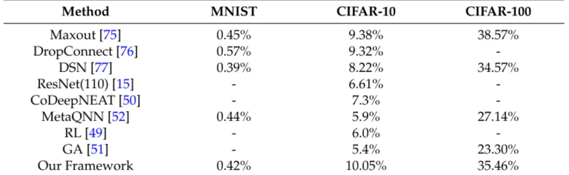
We compare the performance of our approach with state-of-the-art results and recent works on architecture search on three datasets. As seen in Table5, we achieve competitive performance on the MNIST dataset in comparison to the state-of-the-art results, with an error rate 0.42%. The results on CIFAR-10 and CIFAR-100 are obtained after applying data augmentation. Recent architecture search techniques [49–52] show good results; however, these promising results were only possible with substantial computation resources and a long execution time. For example, GA [51] used genetic algorithms to discover the network architecture for a given task. Each experiment was distributed to over 250 parallel workers. Ref. [49] used reinforcement learning (RL) to tune a total of 12,800 different architectures to find the best on CIFAR-10, and the task took over three weeks. However, our framework uses only three workers and requires tuning an average of 260 different CNN architectures in around one day. It is possible to run our framework on a single computer. Therefore, our approach is comparable to the state-of-the-art results on CIFAR-10 and CIFAR-100, because our results require significantly fewer resources and less processing time. Some methods such as Residential Networks (ResNet) [15] achieve state-of-the-art results because the structure is different than a CNN. However, it is possible to implement our framework in ResNet to find the best architecture.
Table 5.Error rate comparisons with state-of-the-art methods and recent works on architecture design search. We report results for CIFAR-10 and CIFAR-100 after applying data augmentation and results for MNIST without any data augmentation.
Method MNIST CIFAR-10 CIFAR-100
Maxout [75] 0.45% 9.38% 38.57% DropConnect [76] 0.57% 9.32% -DSN [77] 0.39% 8.22% 34.57% ResNet(110) [15] - 6.61% -CoDeepNEAT [50] - 7.3% -MetaQNN [52] 0.44% 5.9% 27.14% RL [49] - 6.0% -GA [51] - 5.4% 23.30% Our Framework 0.42% 10.05% 35.46%
To test the robustness of the selection of the training sample, we compared a random selection against RMHC for the same sample size; we found that RMHC achieved better results by about 2%. We found that our new objective function is very effective in guiding a large search space into a sub-region that yields a final, high-performing CNN architecture design. Pooling layers and large strides show a poor visualization, so our framework restricts the placement of pooling layers: It does not follow every convolutional layer with a pooling layer, which shrinks the size of the strides. Moreover, this results in increased depth. We found that the framework allows navigation through a large search space without any restriction on depth until it finds a promising CNN architecture. Our framework can be implemented in other problem domains where images and visualization are involved, such as image registration, detection, and segmentation.
6. Conclusions
Despite the success of CNNs in solving difficult problems, optimizing an appropriate architecture for a given problem remains a difficult task. This paper addresses this issue by constructing a
Entropy2017,19, 242 17 of 20
framework that automatically discovers a high-performing architecture without hand-crafting the design. We demonstrate that exploiting the visualization of feature maps via deconvnet in addition to the error rate in the objective function produces a superior performance. To address high execution time in exploring numerous CNN architectures during the optimization process, we parallelized the NMM in conjunction with an optimized training sample subset. Our framework is limited by the fact that it cannot be applied outside of the imaging or vision field because part of our objective function relies on visualization via deconvnet.
In our future work, we plan to implement our framework on different problems in the context of the images. We will also explore cancellation criteria to discover and avoid evaluating poor architectures, which will accelerate the execution time.
Acknowledgments:This research work was funded in part by the Saudi Cultural Mission (SACM). The cost of publishing this paper was funded by the University of Bridgeport, CT, USA.
Author Contributions: This research is part of Saleh Albelwi Ph.D. dissertation work under the supervision Ausif Mahmood. All authors conceived and designed the experiments; S. Albelwi performed the experiments. Manuscript was written by S. Albelwi; A. Mahmood reviewed and approved the final manuscript.
Conflicts of Interest:The authors declare no conflict of interest. References
1. Farabet, C.; Couprie, C.; Najman, L.; LeCun, Y. Learning hierarchical features for scene labeling.IEEE Trans. Pattern Anal. Mach. Intell.2013,35, 1915–1929. [CrossRef] [PubMed]
2. Simonyan, K.; Zisserman, A. Very deep convolutional networks for large-scale image recognition.arXiv 2014, arXiv:1409.1556.
3. Krizhevsky, A.; Sutskever, I.; Hinton, G.E. Imagenet classification with deep convolutional neural networks. In Proceedings of the 25th International Conference on Neural Information Processing Systems, Lake Tahoe, NV, USA, 3–6 December 2012; pp. 1097–1105.
4. Kalchbrenner, N.; Grefenstette, E.; Blunsom, P. A convolutional neural network for modelling sentences. arXiv2014, arXiv:1404.2188.
5. Kim, Y. Convolutional neural networks for sentence classification.arXiv2014, arXiv:1408.5882.
6. Conneau, A.; Schwenk, H.; LeCun, Y.; Barrault, L. Very deep convolutional networks for text classification. arXiv2016, arXiv:1606.01781.
7. Hubel, D.H.; Wiesel, T.N. Receptive fields and functional architecture of monkey striate cortex.J. Physiol. 1968,195, 215–243. [CrossRef] [PubMed]
8. Sermanet, P.; Eigen, D.; Zhang, X.; Mathieu, M.; Fergus, R.; LeCun, Y. Overfeat: Integrated recognition, localization and detection using convolutional networks.arXiv2013, arXiv:1312.6229.
9. Bengio, Y. Learning deep architectures for AI.Found. Trends Mach. Learn.2009,2, 1–127. [CrossRef] 10. Deng, J.; Dong, W.; Socher, R.; Li, L.J.; Li, K.; Li, F. Imagenet: A large-scale hierarchical image database.
In Proceedings of the IEEE Conference on Computer Vision and Pattern Recognition, Miami, FL, USA, 20–25 June 2009; pp. 248–255.
11. Srivastava, N.; Hinton, G.E.; Krizhevsky, A.; Sutskever, I.; Salakhutdinov, R. Dropout: A simple way to prevent neural networks from overfitting.J. Mach. Learn. Res.2014,15, 1929–1958.
12. Liu, Y.; Racah, E.; Correa, J.; Khosrowshahi, A.; Lavers, D.; Kunkel, K.; Wehner, M.; Collins, W. Application of deep convolutional neural networks for detecting extreme weather in climate datasets. arXiv2016, arXiv:1605.01156.
13. Esteva, A.; Kuprel, B.; Novoa, R.A.; Ko, J.; Swetter, S.M.; Blau, H.M.; Thrun, S. Dermatologist-level classification of skin cancer with deep neural networks.Nature2017,542, 115–118. [CrossRef] [PubMed] 14. Zeiler, M.D.; Fergus, R. Visualizing and understanding convolutional networks. In Proceedings of the
European Conference on Computer Vision, Zurich, Switzerland, 6–12 September 2014; pp. 818–833. 15. He, K.; Zhang, X.; Ren, S.; Sun, J. Deep residual learning for image recognition.arXiv2015, arXiv:1512.03385. 16. Srivastava, R.K.; Greff, K.; Schmidhuber, J. Training very deep networks. In Proceedings of the 28th International Conference on Neural Information Processing Systems, Montreal, QC, Canada, 7–12 December 2015; pp. 2377–2385.